Exploring effects of strong interactions in enhancing masses of dynamical origin

Abstract

A previous study of the dynamical generation of masses in massless QCD is considered from another viewpoint. The quark mass is assumed to have a dynamical origin and is substituted by a scalar field without self-interaction. The potential for the new field background is evaluated up to two loops. Expressing the running coupling in terms of the scale parameter $\mu$, the potential minimum is chosen to fix $m_{top}=175$ $GeV$ when $\mu_{0}=498$ $MeV$. The second derivative of the potential predicts a scalar field mass of $126.76$ $GeV$. This number is close to the value $114$ $GeV$ which, preliminary data taken at CERN, suggested to be associated with the Higgs particle. However, the simplifying assumptions limit the validity of the calculations done, as indicated by the large value of $\alpha=\frac{g^{2}}{4\pi}=1.077$ obtained. However, supporting statements about the possibility of improving the scheme come from the necessary inclusion of weak and scalar field couplings and mass counterterms in the renormalization procedure, in common with the seemingly needed consideration of the massive W and Z fields, if the real conditions of the SM model are intended to be approached.

I Introduction

The understanding of the hierarchy in the particle mass spectrum remains to be a central question in High Energy Physics nambu ; fritzsch ; coleman ; bardeen ; miransky ; minkowski ; clague .  In former works we had been considering an alternative perturbation expansion for QCD, in which quark and gluon condensates are incorporated in the free vacuum state for afterwards determine the alternative modified Wick expansion mpla ; prd ; epjc ; epjc1 ; jhep ; epjc2 ; hoyer ; hoyer1 ; hoyer2 ; epjc19 .  A main motivation for this study was the wonder about what could result to be the final strength of dynamically generated quark condensates in massless QCD, a theory in which the free vacuum is highly degenerated, and the underlying forces are the strongest ones in Nature coleman .  Another source of interest was to imagine that the modified expansion could represent a foundation of the similarities of the particle mass spectrum with the ones in superconductor systems, as stressed in Ref. fritzsch ; fritzsch1 . This possibility was indicated, on one side, by the fact that the employed fermion condensate free vacuums closely resembled the similar ”squeezed” states structure of the usual BCS wavefunctions in standard superconductivity theory prd . In  Ref. mpla ; prd ; epjc ; epjc1 ; jhep ; epjc2 ; epjc09 some indications about the possible dynamic generation of quark and gluon condensates had been obtained. However, although the evaluated corrections signaled the dynamical generation of the quark condensate parameter, the vacuum energy turned out to be unbounded from below as a function of this quantity in the two loop calculation done in epjc09 . In this same work we restricted the discussion to the simpler case in which there is only quark condensates present in the system. In this situation, the Green’s functions generating functional $Z$ was transformed to a more helpful form, as the same functional integral associated to massless QCD, in which all the effects of the quark condensates are now embodied in only one additional vertex having two quark and two gluon legs. This representation allows to systematize the diagrammatic expansion. In particular it permits to implement the dimensional transmutation effect. The evaluation of next corrections of the potential in order to search for its stabilizing minimum are expected to be further considered. These next corrections, however, show complications for their calculation due to the taquionic character of the ladder approximation for the gluon propagator employed up to now in the evaluations.

In the present work we intend to also start examining the same problem from another angle. The first motivation for doing this came after taking into account that the fermion condensation properties of massless QCD should be described by the effective action for composite operators, in particular the $\overline{\Psi}(x)\Psi(x)$ one effcomp1 ; effcomp2 .  We also plan to consider this approach in the near future. However, a closely related, but simpler to tract task, can be to consider the same generating functional of the $\overline{\Psi}(x)\Psi(x)$ insertions for massless QCD (which Legendre transform  determine the mean $\left\langle\overline{\Psi}(x)\Psi(x)\right\rangle),$ but in which the sources $J(x)$ in place of being external and auxiliary ones, are chosen to be dynamical quantities.  This procedure then, amounts to investigate the same question about the dynamic generation of the quark masses, but through the interaction of massless QCD with another dynamical system.  At this point, it can be observed that it is an increasingly accepted viewpoint, that all the coupling constants and mass parameters can have a dynamic origin witten ; polchinski . Then, two possibilities for the physical relevance of introducing the dynamical mass come to the mind. One is the interaction with an scalar field in which the quark mass (source) is given through Yukawa terms.  The same SM is included in this case, but for the restrictive condition of the scalar field system to show a negative squared mass musolf ; casas1 ; nielsen .  Another interesting situation of a dynamical quark mass, comes from superstring theory, where it is known that the fluxes in the compactified spaces generalizing the Kaluza-Klein approach, can produce massive terms for fermions in their low energy effective actions. This happens by example, in Type IIB superstrings witten .   In this work we decided to consider the first variant and assume, for the sole sake of simplicity, that the quark interacts with a scalar field which mass and potential terms in the classical Lagrangean are both zero. As it will be seen, We plan to delete this calculational restrictions, as a consequence of the obtained conclusions.  The initial exploration consists in evaluating the effective potential of massless QCD as a function of the ”mass” field background up to the two loops approximation. This is decided with the aim of answering the question about whether or not at some special and reasonable renormalization point conditions, the strong QCD interactions becomes able to generate a minimum of the potential determining the measured top quark mass of nearly $m_{top}=173$  $GeV.$

The results for the one loop potential indicate that this contribution becomes unbounded from below at high ”mass” field values. The two loop terms, even after assumed to have small coefficients, dominate at high field values, determining a minimum at some given mass value depending on the parameters. This minimum is higher than $m_{top}$ if the strong coupling is chosen to be small, that is, not in the infrared region. It is an interesting fact, that this minimum seems to be related with the known existence of a second minimum of the Higgs potential at large values of the Higgs field. This high field minimum is precisely produced by the contribution of the Yukawa term for the top quark, which has the same form as the one considered here musolf ; casas1 ; nielsen . This high field minimum appears in the evaluations associated to the Standard Model (SM), at high energy renormalization point where the strong interactions are small. However, as it will be remarked below, the initial evaluations done here suggest an alternative picture for implementing the symmetry breaking in the SM model in which a hidden relevance of the strong coupling can exists.

The work proceeds by evaluating the potential at the values of the running coupling satisfying the one loop RG dependence on the scale parameter $\mu$ by assuming the estimate $\Lambda_{QCD}=217$ $MeV.$  In this circumstance, the minimum of the effective potential as a function of the ”mass” field can be fixed at $m_{top}\approx 175$ $GeV,$ after the scale parameter is chosen at the value $\mu_{0}=498$ $MeV.$ In addition, the second derivative of the effective potential in its minimum at $\phi\sim 175$ $GeV$,  gives a result of $\ \ m_{\phi}$ $\sim 126.76$ $GeV$ for the scalar field mass. It should be noted that the resulting value of the coupling $\alpha=1.077$ becomes neatly inside the non perturbative region, and therefore the validity of the evaluated quantities in this first exploration is not assured. However, after including the ”mass” field in a two loop RG improvement of the evaluated effective action, it is imaginable that the potential can be made RG invariant up to higher $\mu$ scales, where the strong coupling becomes low, but the scalar and weak ones are enhanced. Therefore, the results could become able to imply the generation of the top quark mass from a model in which the mass has a dynamical origin. This possibility seems feasible after taking in mind some considerations: 1) That a $\lambda\phi^{4}$ counterterm should be forced to be included after a consistent renormalization procedure is developed. Therefore, further terms of similar analytical structure as functions of the ”mass” field are expected to appear in the improvement of the simple analysis done here. In particular the coefficient of the squared logarithm of this field  terms (which makes the potential bounded from below) should become a linear combination of $g_{0}^{2}$ and $\lambda$. 2) Further, it can be noticed that our aim is to expect a contact with the real SM model, where the scalar field is in fact a doublet and tightly interacts with the also very massive Z and W bosons. Therefore, for the model to becomes realist, it seem necessary to also include the contributions to the effective action of all such additional modes. The large masses of the Z and W particles should determine appreciable contributions to the potential, and the non asymptotically free dependence with the scale $\mu$ of the weak coupling can be expected to help in assuring the renormalization group invariance of the potential as described in the next point.

3) Thus, since the gauge field coupling is asymptotically free, but the weak and scalar ones are not, it can be expected that under a reduction of the scale $\mu$, the $g_{0}^{2}$ and the non asymptotically $\lambda$ and weak couplings can interchange their roles in maintaining the RG invariance of the potential. Therefore, assumed this effect to occurs up to a point in which the QCD coupling is able to dominate, it can be possible to interpret that the symmetry breaking effect in the SM model might be also considered as strongly linked with the strong interactions dynamics of QCD. As remarked, the strong links that the RG could imposes on both kind of fields interacting through the chirality breaking Yukawa terms, could be the main element determining the above mentioned hidden role the strong interactions. Curious and perhaps related deep links between the gauge theories and Higgs model were also identified before in Ref. nielsen .

Therefore, in general terms, the results suggest the possibility to reformulate the SM model by deleting the negative mass in the classical potential of the Higgs field, and fixing the dynamically generated minimum of the scalar ”mass” field to determine the value of the top quark mass.  The further investigation of this question along the proposed lines is expected to be considered elsewhere.

Finally, the above remarks also leads to conceive that the quark masses could be in essence, dynamically generated by the strong forces, through the Yukawa terms (associated to their fermion fields components) which are generated by the fluxes in the low energy action of superstring theories.   In this view the Higgs field could be realized by the flux created mass factors of the top quark chiral condensate operator in the low energy actions.

The work proceeds as follows. In Section II the action and the notations to be employed for the generating functional of massless QCD in interaction with the ”mass” scalar field will be defined.  Section II will consider the MS evaluations of the one and too loop contribution to the effective potential. In Section IV a discussion about the above remarks, following from the examination of the evaluated potential will be presented. The results are again commented in the Summary.

II QCD interacting with a dynamical ”mass” field

Let us consider the Green’s functions generating functional   $Z$ describing massless QCD fields in interaction with a scalar field $\phi,$ which is assumed to be real for the sake of simplicity. The functional has the form

$$Z[j,\eta,\overline{\eta},\xi,\overline{\xi},\rho]=\frac{1}{\mathcal{N}}\int\mathcal{D}[A,\overline{\Psi},\Psi,\overline{c},c,\phi]\exp[i\text{ }S[A,\overline{\Psi},\Psi,\overline{c},c,\phi]],$$ (1)

In this expression, $S$ is the action of the system closely following the conventions of Ref. muta :

$$S =\int dx(\mathcal{L}_{0}\mathcal{+L}_{1}\mathcal{)},$$ (2)

$$\mathcal{L}_{0} =\mathcal{L}^{g}+\mathcal{L}^{gh}+\mathcal{L}^{q}+\mathcal{L}^{\phi},$$ (3)

$$\mathcal{L}^{g} =-\frac{1}{4}(\partial_{\mu}A_{\nu}^{a}-\partial_{\nu}A_{\mu}^{a})(\partial^{\mu}A^{a,\nu}-\partial^{\nu}A^{a,\mu})-\frac{1}{2\alpha}(\partial_{\mu}A^{\mu,a})(\partial^{\nu}A_{\nu}^{a}),$$ (4)

$$\mathcal{L}^{gh} =(\partial^{\mu}\chi^{*a})\partial_{\mu}\chi^{a},$$ (5)

$$\mathcal{L}^{q} =\overline{\Psi}(i\gamma^{\mu}\partial_{\mu})\Psi,$$ (6)

$$\mathcal{L}^{\phi} =\partial^{\mu}\phi\partial_{\mu}\phi,$$ (7)

$$\mathcal{L}_{1} =-\frac{g}{2}f^{abc}(\partial_{\mu}A_{\nu}^{a}-\partial_{\nu}A_{\mu}^{a})A^{b,\mu}A^{c,\nu}-g^{2}f^{abe}f^{cde}A_{\mu}^{a}A_{\nu}^{b}A^{c,\mu}A^{d,\nu}-$$

$$-gf^{abc}(\partial^{\mu}\chi^{*a})\chi^{b}A_{\mu}^{c}+g\overline{\Psi}T^{a}\gamma^{\mu}\Psi A_{\mu}^{a}+\overline{\Psi}\Psi\phi.$$ (8)

The classical action of the scalar field has been also chosen to be self-interaction free and massless. As mentioned in the introduction, this restrictions only constitute an assumption in attempting to simplify the evaluations. It will be expected to be relaxed in improving the present study after implementing a renormalization procedure by incorporating counterterms and additional terms in the action, which can directly lead to masses and scalar field couplings as required by the structure of the divergences. It should be said in advance that this improvement will result to be essential for verifying the preliminary conclusions of this first examination of the problem. Note also that the interaction of the scalar field with $\phi$ is simply a Yukawa term, like the same one for the quarks in the Standard Model.

III One and two loop effective potential of the ”mass” field

Let us consider in this section the evaluations of the contributions to the effective potential $v(\phi)$ which QCD ”creates” on the scalar field $\phi,$ up to the second loop order. The case of homogenous values of $\phi$ will be assumed.

III.1 One loop term 

The analytic expression for the one loop contribution shown in Fig. 1 is given by the classical logarithm of the fermion quark determinant as:

$$\Gamma^{(1)}[\phi] = -V^{(D)}N\int\frac{dp^{D}}{i\text{ }(2\pi)^{D}}Log[Det\text{ }(G_{ii^{\prime}}^{(0)rr^{\prime}}(\phi,p))],$$ (9)

$$D = 4-2\epsilon,$$

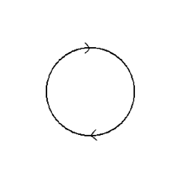
Figure 1: The figure shows the quark one loop correction. The result depends on the scalar ”mass” field $\phi$ through the quark free propagator which is the usual free Green function of QCD, in which the mass is substituted by $\phi$.

where $D$ is the space dimension of dimensional regularization and the free fermion propagator is written in the conventions of Ref.  muta , which will be used throughout this work. Its expression is given by

$$G_{ii^{\prime}}^{(0)rr^{\prime}}(\phi,p) =\delta^{ii^{\prime}}{\Large(}\frac{1}{-p_{\mu}\gamma^{\mu}+\phi}{\Large)}^{rr^{\prime}}$$

$$=-\frac{\delta^{ii^{\prime}}}{p^{2}-\phi^{2}}{\Large(}p_{\mu}\gamma^{\mu}+\phi{\Large)}^{rr^{\prime}}.$$ (10)

Assuming the case of QCD with $SU(N)$ symmetry for N=3, and evaluating the spinor and color traces, the one loop expression can be simplified to the form

$$\Gamma^{(1)}[\phi]=V^{(D)}\frac{N}{2}\int\frac{dp^{D}}{i\text{ }(2\pi)^{D}}Log[(\phi^{2}-p^{2})^{4}].$$

Taking the derivative over $\phi^{2}$ of $\Gamma^{(1)}[\phi]$ allows to write the easily integrable expression

$$\frac{d}{d\text{ }\phi^{2}}\Gamma^{(1)}[\phi]=V^{(D)}2N\int\frac{dp^{D}}{\text{ }(2\pi)^{D}}\frac{1}{(p^{2}+\phi^{2})},$$

which after making use of the formula

$$\int\frac{dp^{D}}{\text{ }(2\pi)^{D}}\frac{1}{(p^{2}+\lambda^{2})}=\frac{\Gamma(1-\frac{D}{2})}{(4\pi)^{\frac{D}{2}}}(\lambda^{2})^{\frac{D}{2}-1},$$ (11)

and integrating the result back over $\phi^{2}$, results in the dimensionally regularized expression

$$\Gamma^{(1)}[\phi] = V^{(D)}\frac{2N\Gamma(1-\frac{D}{2})}{(\frac{D}{2})(4\pi)^{\frac{D}{2}}}(\phi^{2})^{\frac{D}{2}-1}$$ (12)

$$= V^{(D)}\frac{2N\text{ }\Gamma(\epsilon-1)}{(\frac{D}{2})(4\pi)^{2-\epsilon}}(\phi^{2})^{2-\epsilon}.$$

Now, it is possible to divide $\Gamma^{(1)}[\phi]$ by $\frac{V(D)}{\mu^{2\epsilon}}$, in order to obtain the action density. The quantity $\mu$ in the denominator is the dimensional regularization scale parameter, and the divisor $\mu^{2\epsilon},$ which tends to one on removing the regularization, is introduced in order avoid results containing logarithms of quantities having dimension. Then, the one loop Lagrangian density takes the form

$$\gamma^{(1)}[\phi]=\frac{\Gamma^{(1)}[\phi]}{\frac{V(D)}{\mu^{2\epsilon}}}=\frac{2N\text{ }\Gamma(\epsilon-1)}{(\frac{D}{2})(4\pi)^{2-\epsilon}}\phi^{2}(\frac{\phi}{\mu})^{-2\epsilon}.$$ (13)

Further, deleting the pole part of this formula according to the Minimal Substraction rule, and taking the limit $\epsilon\rightarrow 0,$ gives the finite part of the action density as

$$\left[\gamma^{(1)}[\phi]\right]_{finite}=\frac{3\phi^{4}}{8\pi^{2}}(-3+2\gamma+2Log(\frac{\phi^{2}}{2\pi\mu^{2}})).$$ (14)

Finally, the one loop potential energy density is given by the negative of the above quantity

$$v^{(1)}[\phi]=-\frac{3\phi^{4}}{8\pi^{2}}(-3+2\gamma+2Log(\frac{\phi^{2}}{2\pi\mu^{2}})).$$ (15)

It can be noticed that this potential density is unbounded from below for increasing values of the scalar field. This is the main property determining the dynamical generation of the field $\phi$.

III.2 Quark-gluon two loop term

The two loop quark-gluon term to be considered in this subsection is illustrated in Fig. 2.  Again, after evaluating the color and spinor traces its analytic expression can be written as follows

$$\Gamma^{(2)}[\phi]=-V^{(D)}g^{2}(N^{2}-1)\int\frac{dp^{D}dq^{D}}{i^{2}\text{ }(2\pi)^{2D}}\frac{D\phi^{2}-(D-2)p.(p+q)}{q^{2}(p^{2}-\phi^{2})((p+q)^{2}-\phi^{2})},$$ (16)

where $g^{2}$ is the QCD coupling constant in the dimensional regularization scheme, which introduces the scale parameter $\mu$ according to

$$g=g_{0}\text{ }\mu^{2-\frac{D}{2}}=g_{0\text{ }}\mu^{\epsilon}.$$ (17)

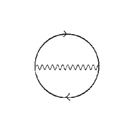
Figure 2: The two loop contribution determined by the strong interaction. Again the $\phi$ dependence of the result is introduced though the free quark propagator.

After  symmetrizing the expression  of $\Gamma^{(2)}[\phi]$ under the change of sign in the momentum $q$, by means of the integration variable shift $\ p\rightarrow p-\frac{q}{2},$ and the use of the identity

$$p^{2}=(p+\frac{q}{2})^{2}-\phi^{2}+\phi^{2}-\frac{q^{2}}{4}-q.p,$$ (18)

the  quark-gluon term may be written as the sum of two contributions of the form

$$\Gamma^{(2)}[\phi]=\Gamma^{(2.1)}[\phi]+\Gamma^{(2,2)}[\phi],$$ (19)

in which $\Gamma^{(2.1)}[\phi]$ and $\Gamma^{(2,2)}[\phi]$ have the formulae

$$\Gamma^{(2,1)}[\phi] = -V^{(D)}2\phi^{2}g^{2}(N^{2}-1)\int\frac{dk_{1}^{D}dk_{2}^{D}}{i^{2}\text{ }(2\pi)^{2D}}\frac{1}{k_{1}^{2}(k_{2}^{2}-\phi^{2})((k_{1}+k_{2})^{2}-\phi^{2})}$$ (20)

$$= -V^{(D)}\frac{2\phi^{2}g^{2}(N^{2}-1)}{i^{2}\text{ }(2\pi)^{2D}}J_{111}(0,\phi,\phi)$$

$$\Gamma^{(2,2)}[\phi] = -V^{(D)}\frac{(D-2)g^{2}(N^{2}-1)}{2i^{2}(2\pi)^{2D}}{\LARGE(}\int dk_{1}^{D}\frac{1}{k_{1}^{2}-\phi^{2}}{\LARGE)}^{2},$$ (21)

where, the master two loop integral $J_{111}(0,\phi,\phi)$ ,  was evaluated in Ref. tausk , and its explicit form for our particular arguments is:

$$J_{111}(0,\phi,\phi) = \int dk_{1}^{D}dk_{2}^{D}\frac{1}{k_{1}^{2}(k_{2}^{2}-\phi^{2})((k_{1}+k_{2})^{2}-\phi^{2})}$$ (22)

$$= -\frac{A(\epsilon)\pi^{4-2\epsilon}}{\epsilon^{2}}(\phi^{2})^{1-2\epsilon},$$

$$A(\epsilon) = \frac{(\Gamma(1+\epsilon))^{2}}{(1-\epsilon)(1-2\epsilon)}.$$ (23)

Then, it is possible to write for $\Gamma^{(2,1)}$

$$\Gamma^{(2,1)}[\phi]=-\frac{V^{(D)}2g_{0}^{2}\mu^{2\epsilon}(N^{2}-1)}{\text{ }(2\pi)^{8-4\epsilon}}\frac{A(\epsilon)\pi^{4-2\epsilon}}{\epsilon^{2}}\phi^{4}(\phi^{2})^{-2\epsilon}.$$ (24)

In the case of $\Gamma^{(2,2)},$ the result is the square of the one loop integral in equation (11), which leads to

$$\Gamma^{(2,2)}[\phi]=V^{(D)}\frac{g_{0}^{2}\mu^{2\epsilon}(N^{2}-1)2(1-\epsilon)}{\text{ }2(2\pi)^{8-4\epsilon}}\pi^{4-2\epsilon}(\Gamma(\epsilon-1))^{2}\phi^{4}(\phi^{2})^{-2\epsilon}.$$ (25)

Again dividing by $\frac{V(D)}{\mu^{2\epsilon}}$ to evaluate the action densities gives for the corresponding terms

$$\gamma^{(2,1)}[\phi] = \frac{\Gamma^{(2,1)}[\phi]}{\frac{V(D)}{\mu^{2\epsilon}}}=-v^{(2,1)}[\phi]$$ (26)

$$= -\frac{2g_{0}^{2}(N^{2}-1)}{\text{ }(2\pi)^{2D}}\frac{A(\epsilon)\pi^{4-2\epsilon}}{\epsilon^{2}}\phi^{4}(\frac{\phi^{2}}{\mu^{2}})^{-2\epsilon},$$

and

$$\gamma^{(2,2)}[\phi] = \frac{\Gamma^{(2,2)}[\phi]}{\frac{V(D)}{\mu^{2\epsilon}}}=-v^{(2,2)}[\phi]$$ (27)

$$= V^{(D)}\frac{g_{0}^{2}\mu^{2\epsilon}(N^{2}-1)2(1-\epsilon)}{\text{ }2(2\pi)^{8-4\epsilon}}\pi^{4-2\epsilon}(\Gamma(\epsilon-1))^{2}\phi^{4}(\phi^{2})^{-2\epsilon},$$

which define the potential energy densities $v^{(2,1)}[\phi]$ and $v^{(2,2)}[\phi]$ as their negatives.  After substracting the divergent poles, taking the limit $\epsilon\rightarrow 0$ and numerically evaluating all the constants in order to simplify the view of the resulting expression, the total quark gluon two loop finite contribution to the energy density reduces to the form

$$v^{(2)}[\phi] = 5.34687\times 10^{-5}\phi^{4}{\LARGE(}1227.16+474.276\text{ }g_{0}^{2}-$$ (28)

$$12.0(\text{ }29.6088+13.5253\text{ }g_{0}^{2})\text{ }Log(\frac{\phi^{2}}{\mu^{2}})+$$

$$12.0\text{ }g_{0}^{2}\text{ }(Log(\frac{\phi^{2}}{\mu^{2}}))^{2}{\LARGE).}$$

It can be seen that the leading logarithm term is positive, indicating that the contribution of the usual QCD diagrams to the potential up to the two loop approximation becomes bounded from below as a function of $\phi$.

III.3 Scalar-quark two loop term

Finally, in this section let us present the two loop term being associated to the quark-scalar loop illustrated in Fig. 3 . This calculation is similar to the previous one, but simpler, due to the lack of spinor and color structures in the vertices.

Figure 3: The diagram corresponding to the radiative corrections of the ”mass” field $\phi$ in the two loop order.

This graph analytic expression can be written in the following way

$$\Gamma_{Y}^{(2)}[\phi]=V^{(D)}2N\int\frac{dp^{D}dq^{D}}{i^{2}\text{ }(2\pi)^{2D}}\frac{p^{2}-\frac{q^{2}}{4}+\phi^{2}}{q^{2}((p+\frac{q}{2})^{2}-\phi^{2})((p-\frac{q}{2})^{2}-\phi^{2})},$$ (29)

which in a very close manner as in the previous subsection, can be represented as follows

$$\Gamma_{Y}^{(2)}[\phi] = V^{(D)}\frac{4N}{i^{2}\text{ }(2\pi)^{2D}}J_{111}(0,\phi,\phi)$$ (30)

$$-V^{(D)}N{\LARGE(}\int\frac{dk_{1}^{D}}{i(2\pi)^{D}\text{ }}\frac{1}{k_{1}^{2}-\phi^{2}}{\LARGE)}^{2}$$

$$= \frac{V^{(D)}4N}{\text{ }(2\pi)^{8-4\epsilon}}\frac{A(\epsilon)\pi^{4-2\epsilon}}{\epsilon^{2}}\phi^{4}(\phi^{2})^{-2\epsilon}$$

$$-V^{(D)}\frac{N}{\text{ }(2\pi)^{8-4\epsilon}}\pi^{4-2\epsilon}(\Gamma(\epsilon-1))^{2}\phi^{4}(\phi^{2})^{-2\epsilon}.$$

The division by the volume $\frac{V(D)}{\mu^{2\epsilon}}$ allows to write for the action density and its negative: the potential one, the formula

$$\gamma_{Y}^{(2)}[\phi] = -v_{Y}^{(2)}[\phi]$$ (31)

$$= \frac{4N}{\text{ }(2\pi)^{8-4\epsilon}}\frac{A(\epsilon)\pi^{4-2\epsilon}}{\epsilon^{2}}\phi^{4}(\frac{\phi^{2}}{\mu^{2}})^{-2\epsilon}$$

$$-\frac{N}{\text{ }(2\pi)^{8-4\epsilon}}\pi^{4-2\epsilon}(\Gamma(\epsilon-1))^{2}\phi^{4}(\frac{\phi^{2}}{\mu^{2}})^{-2\epsilon}.$$

The substraction of the divergent pole part in $\epsilon$, passing to the limit $\epsilon\rightarrow 0$ and numerically evaluating the appearing constants, gives for the potential density

$$v_{Y}^{(2)}[\phi]=-0.0000601522\text{ }m^{4}\left(332.744-123.833Log[\frac{m^{2}}{\mu^{2}}]+12.0\,Log[\frac{m^{2}}{\mu^{2}}]^{2}\right).$$ (32)

It can be noted that this contribution, being a two loop one, also includes a squared logarithm term. However, its sign is contrary to the one appearing in the quark gluon loop.

IV  Discussion

Let us consider the sum of all the just evaluated contributions to the potential energy density, defining it as the function $v(\phi)$. Its expression is a combination of terms of the form $\phi^{4}$, $\phi^{4}Log(\frac{\phi}{\mu})$ and $\phi^{4}(Log(\frac{\phi}{\mu}))^{2}$, with coefficients that only depend on the strong coupling $g_{0}$ in the present first analysis. Then, in order to approach the physical situation, we evaluated the potential $v(\phi)$ at the values of $g_{0}$ satisfying the one loop formula for the running coupling constant muta

$$g_{0}(\mu,\Lambda_{QCD})=2\sqrt{\frac{2}{7}}\pi\sqrt{\frac{1}{Log(\frac{\mu}{\Lambda_{QCD}})}}.$$ (33)

The $\Lambda_{QCD}$ constant was chosen to be the estimate $\Lambda_{QCD}=0.217\,\,GeV$. Next, we studied the potential curves in order to examine the behavior of their minimum as functions of $\phi$, when the scale $\mu$ is changed. It follows that when the strong coupling starts to increase as the scale diminish down to one $GeV$, the value of $\phi$ at the minima, which determines the quark mass also decreases. For the particular value of $\mu=0.498\,\,GeV$ , the potential curve is shown in Fig.  4.

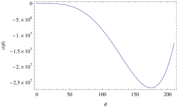
Figure 4: The effective potential for the ”mass” field $\phi$ for the value of the scale $\mu$ determining that the value of $\phi$ taken at the minimum potential, is approximately equal to the top quark mass $m_{top}~{}175\,\,GeV$. An interesting outcome is that the second derivative at the minimum is $m_{\phi}=126.76\,\,GeV$, which is close to the energy $114$ $GeV$, at which some low statistic data measured at ALEPH experiment at CERN years ago, led to suspect its link with the Higgs mass. However, in the simplified model in this work, the scale $\mu$ allowing the top mass fixation is within the non perturbative infrared region: $\mu=0.498\,\,GeV$, which gives a coupling value $\alpha=\frac{g_{0}^{2}}{4\pi}=1.077$. Thus, the described in the text improvements of the treatment are needed for establishing the possibility of fixing the observed value of the top mass in the scheme, and with it, the $126.76\,\,GeV$ estimation of the Higgs particle mass.

The particular value of $\mu$ chosen, fixes the position of the minimum at a ”mass” field $\phi$ defining a quark mass of $~{}175$ $GeV$. The set of parameters for this curve are

$$\mu = 0.498\,\,GeV,$$ (34)

$$g_{0} = 3.684\,\,\,\,(\alpha=\frac{(g_{0})^{2}}{4\pi}=1.077),$$ (35)

$$\Lambda_{QCD} = 0.217\,\,GeV.$$ (36)

An interesting outcome is the fact that the squared root of the second derivative of the potential curve in Fig. 1, estimates for the mass of $\phi$ the value $m_{\phi}=126.76$ $GeV$. It can be remarked that this energy is close to the value of $114$ $GeV$ that years ago appeared as signaling the presence of some low statistic experimental data at CERN, and which were considered as perhaps being related with the Higgs particle. This outcome, however, can not yet be validated, as consequence of the resulting high value of the strong coupling obtained. This elevated value might limit the validity of the two loop and simplifying approximations employed here. However, as remarked in the introduction, there exist additional circumstances that indicate the possibility that the picture remains valid after including renormalization and extending the model in a consistent way. Let us recall here a resume of these remarks: After implementing a renormalization procedure, a $\lambda\phi^{4}$ term should necessarily be added to the Lagrangian (as a well as mass one of the form $m^{2}\phi^{2}$ ). This generalization of the here considered simplified massless and non self-interacting form of the scalar field Lagrangian, automatically should lead to additional coefficients in the logarithmic expansion of the evaluated potential. Further, in order for the extended theory to approach the physical situation in nature, it seems necessary to also incorporate, at least the also very massive Z and W bosons and the weak interactions among these fields. After that, in the same two loop approximation considered here, the coefficient, let us call it $f$, of the bounding from below squared logarithm term $(Log(\frac{\phi^{2}}{\mu^{2}}))^{2}$ can be expected have the form

$$f=a_{1}\text{ }g_{0}^{2}+a_{2}\lambda+a_{3}\text{ }g_{W}^{2}.$$

That is, as a linear function $g_{0}^{2}$, $\lambda$ and the squared weak coupling $g_{W}^{2}$. Since the $a_{1}$ factor is positive as evaluated here,  in case that $a_{2}\lambda+a_{3}\text{ }g_{W}^{2}$ results to be also positive,  the minimum of the potential at the mass of the top quark, has the chance of to be implemented at a larger scale $\mu.$ This possibility follows from the fact that, although $g_{0}$ will diminish after increasing $\mu,$ due to its asymptotically free character, the weak coupling $g_{W}$ and the scalar field one $\lambda$ should be expected to grow because they are non asymptotically free. Therefore, this circumstance can be expected to help in imposing the value of the observed value of the top mass at a higher value of the $\mu$ scale. If this phenomenon occurs, it can be interpreted as a ”trading” of the roles of the weak interaction fields and the strong interaction gauge fields upon passing from a high energy scale to the infrared one.  Thus, when working the perturbative theory at the infrared scale, the Higgs mean field, and with it the top, W and Z masses, can then appear as generated by the Yukawa interaction in combination with the strong forces of the quarks and gauge fields. We expect to be able to support this picture in the extension of this work.

At this point is of interest to observe that the appeared single minimum seems to be related with the known existence of a second minimum of the Higgs potential laying at large values of the Higgs field. This minimum is recognized to be produced precisely by the contribution of the top quark Yukawa term, which is of the same form of the one considered here musolf ; casas1 ; nielsen .  Clearly, if the strong coupling is fixed at the perturbative scale, the here obtained minimum will be shift to very high energies due to the decreasing of the running coupling.

In conclusion, the remarks in this Section, support the possibility that the inclusion of the usual ”$\lambda\phi^{4}"$ coupling for the ”mass” field in the present discussion, but retaining a positive value of its mass, in conjunction with the incorporation of the weak interaction couplings and the Z and W fields, could allow the fixing of the value of top quark mass at $175$ $GeV$, but at higher renormalization scale $\mu$. Note that after this generalization, the structure of the leading logarithm terms contributing to the potential will be similar, and moreover, the unbounded one loop correction is not ruled out that could be able to dominate the terms being linear in the logarithm of $\phi$. Therefore, the fixation of the position of the minimum of the potential at the observed mass of the top quark, but at a higher scale $\mu$, could be eventually again approximately furnish a reasonable estimate for the Higgs mass. The success in this task could lead to a modification of the SM in which the so called second Higgs minimum could substitute the classically imposed one in defining the SM ground state. We expect to present elsewhere the results of a current examination of these issues.

V Summary

Previous investigations about the dynamical generation of large quark masses in a modified version of PQCD were continued here but starting from another viewpoint. For this purpose the mass parameter of the quarks in QCD (or equivalently, a constant source in the generating functional for the quark condensate composite operator in massless QCD) is supposed to be a dynamical quantity. Examples of such situation are the same Yukawa interaction in the SM model and the masses generated by fluxes within compactified spaces in superstring theories.  A simple model of a real scalar field without self-interaction is adopted in the initial exploration done here. The effective action of massless QCD as a function of the introduced ”mass” field background, the strong coupling $g_{0}$ and the scale parameter $\mu$, is calculated up to two loops by employing the MS scheme. After imposing the one loop renormalization group (RE) expression for $g_{0}$ as a function of $\mu$ and choosing $\Lambda_{QCD}=217$ $MeV,$ the single minimum of the evaluated effective potential can be fixed at a scalar field value approximately equal to the top quark mass $m_{top}\approx 175$ $GeV,$ for the scale parameter at $\mu_{0}=498$ $MeV.$ The second derivative of the effective potential gives a scalar field mass of $126.76$ $GeV$. This value is close to the energy at which some insufficient experimental data taken at ALEPH experiment at CERN years ago, suggested that might be associated with the Higgs particle. However, in this first view of the problem, the here employed two loop expansion is yet inaccurate due to the large value of the coupling $\alpha=\frac{g_{0}^{2}}{4\pi}=1.077$. However, the identified possibility motivates the search for validating the analysis. This task seems promising by developing a full renormalization scheme including counterterms, the also very massive modes of the Z and W particles and a RG improvement of the effective potential to be invariant up to a higher renormalization scale. In this sense the following possibility was here identified. Let us consider the introduction of the usual $\lambda\phi^{4}$ coupling for the ”mass” field in the present discussion. It should be noted that it will automatically enter in the consistent renormalization scheme to be introduced. Even a positive mass value of the renormalized Lagrangian mass of $\phi$ should be taken into account. Moreover, let us also introduce the contributions of the W and Z particles and their associated weak couplings. Then, these modifications seem that could be able to allow the fixing of the top quark mass, in a similar way as it was done here, but now at a higher energy scale $\mu$ at which perturbation theory can be valid. This is suggested because now there can appear further bounded from below squared logarithm terms coming from the contributions of the Z,W and scalar four legs vertices. Since the $g_{0}^{2}$ behavior is asymptotically free, but the weak and scalar couplings are not, their influence upon increasing $\mu$, could result to be opposite. Then, it might happens they compensate between them, allowing in this way to fix the minimum of the potential at the same $m_{top}=175$  $GeV$ value, but now at a higher $\mu$ scale. The verification of this idea will support the detection of a Higgs scalar particle near the energy value $m_{Higgs}=126.76$ $GeV$, which the present exploratory study identified. We expect to consider these possibilities in the coming extension of the work.

It was also underlined, that the discussion seems to be closely related with the known existence of a second minimum of the Higgs potential at large values of the Higgs field. This second minimum is recognized to be created precisely by the contribution of the Yukawa term for the top quark, which is of the same form as the one considered here musolf ; casas1 ; nielsen .

In concluding, it can be also remarked that the discussion also motivates the speculative idea about that the Higgs field could be realized as a dynamical ”mass” scalar field defined by the fluxes, which naturally appears in the Yukawa terms of the low energy effective action in superstring theories.

- (1) Y. Nambu and G. Jona-Lasinio, Phys. Rev. 122, 345 (1961).
- (2) H. Fritzsch, Nucl. Phys. B155, 189 (1979).
- (3) S. Coleman and E. Weinberg, Phys. Rev. D7, 1888 (1973).
- (4) W. A. Bardeen, C. T. Hill and M. Lindner, Phys. Rev. D41, 1647 (1990).
- (5) V.A. Miransky, in Nagoya Spring School on Dynamical Symmetry Breaking, ed. K. Yamawaki, World Scientific (1991).
- (6) H. Fritzsch and P. Minkowski, Phys. Rep. 73, 67 (1981).
- (7) D. E. Clague and G. G. Ross, Nucl. Phys. B364, 43 (1991).
- (8) A. Cabo, S. Peñaranda and R. Martínez, Mod. Phys. Lett. A10, 2413 (1995).
- (9) M. Rigol and A. Cabo, Phys. Rev. D62, 074018 (2000).
- (10) A. Cabo and M. Rigol, Eur. Phys. J. C23, 289 (2002).
- (11) A. Cabo and M. Rigol, Eur. Phys. J. C47, 95 (2006).
- (12) A. Cabo and D. Martinez-Pedrera, Eur. Phys. J. C47, (2006).
- (13) P. Hoyer, NORDITA-2002-19 HE (2002), e-Print Archive: hep-ph/0203236 (2002).
- (14) P. Hoyer, Proceedings of the ICHEP 367-369, Amsterdam (2002), e-Print Archive: hep-ph/0209318.
- (15) P. Hoyer, Acta Phys. Polon. B34, 3121 (2003). e-Print Archive: hep-ph/0304022.
- (16) A. Cabo, Eur. Phys. J. C55, 85 (2008).
- (17) A. Cabo, JHEP 04, 044 (2003).
- (18) A. Cabo Montes de Oca, N. G. Cabo Bizet and A. Cabo-Bizet, Eur. Phys. Jour. C64, 113 (2009).
- (19) T. Muta, Foundations of Quantum Chromodynamics, World Scientific Lectures Notes in Physics, Vol. 5, (1987).
- (20) M. Gonderinger, Y. Li, H. Patel and M. Ramsey-Musolf, JHEP 1001: 053 (2010).
- (21) J. A. Casas, J. R. Espinosa and M. Quiros, Phys. Lett. B382, 374 (1996).
- (22) C. D. Froggatt and H. B. Nielsen, Phys. Lett. B368, 96 (1996).
- (23) M. B. Green, J. H. Schwarz and E. Witten, Superstring theory, Cambridge University Press, 1987.
- (24) J. G. Polchinski, String theory, Cambridge University Press, 1998.
- (25) H. Fritzsch, Nucl. Phys. B (Proc. Suppl.) 40, 121 (1995).
- (26) J. M. Cornwall, R. Jackiw and E. Tomboulis, Phys. Rev. D10, 2448 (1974)
- (27) R. Casalbuoni, S. De Curtis, D. Dominici and R. Gatto, Phys. Lett. B150, 295 (1985).
- (28) J. Fleischer and O. V. Tarasov, Z. Phys. C64, 413 (1994).