Increasing the Reliability of Adaptive Quadrature Using Explicit Interpolants

Abstract

We present two new adaptive quadrature routines. Both routines differ from previously published algorithms in many aspects, most significantly in how they represent the integrand, how they treat non-numerical values of the integrand, how they deal with improper divergent integrals and how they estimate the integration error. The main focus of these improvements is to increase the reliability of the algorithms without significantly impacting their efficiency. Both algorithms are implemented in Matlab and tested using both the “families” suggested by Lyness and Kaganove and the battery test used by Gander and Gautschi and Kahaner. They are shown to be more reliable, albeit in some cases less efficient, than other commonly-used adaptive integrators.

Author’s address: P. Gonnet (gonnetp@inf.ethz.ch), Department of Computer Science, ETH Zentrum, 8092 Zürich, Switzerland.

1 Introduction

Since the publication of the first adaptive quadrature algorithms almost 50 years ago, much has been done and even more has been written on the subject: In 1962 Kuncir [Kuncir (1962)] kicked-off the field with his adaptive Simpson’s rule integrator, which uses – as the name suggests – Simpson’s rule to approximate the integral, bisecting recursively until the difference between the approximation in one interval and that of its two sub-intervals is below the required tolerance. This approach, as simple as it may seem, still lives on, with some minor modifications, as the default integrator quad in MATLAB (added in [The Mathworks (2003)]). quad is itself a modification of Gander and Gautschi’s 2001 adaptsim [Gander and Gautschi (2001)] which is itself a modification of Lyness’ 1970 SQUANK [Lyness (1970)], which is itself almost identical to Kuncir’s original algorithm.

At the time of Kuncir’s publication, McKeeman [McKeeman (1962), McKeeman and Tesler (1963), McKeeman (1963)] and later Forsythe et al. [Forsythe et al. (1977)] extended this approach to use higher-degree Newton-Cotes rules and/or sub-division into more than two sub-intervals.

In 1971, de Boor [de Boor (1971)] introduced the concept of “double adaptivity”, constructing a Romberg T-table [Bauer et al. (1963)] within each sub-interval to approximate the integrand and deciding, at every step, whether to extend the T-table by another row (i.e. increase the order of the quadrature) or to subdivide the interval. This decision was made by using the convergence rates of the columns of the T-table to guess the integrand’s behavior, i.e. “well behaved”, singular, discontinuous or noisy, and apply an adequate strategy for that behavior.

The emergence of more powerful computers and better algorithms (e.g. ref:Golub1969 and ref:Gentleman1972b) for the construction of more complex quadrature rules quickly led to the wider use of Clenshaw-Curtis quadrature rules [Clenshaw and Curtis (1960)], as used by ref:OHara1969 and ref:Oliver1972, and later the use of Gauss quadrature rules and their Kronrod extensions [Kronrod (1965)], first used by ref:Piessens1973 and ref:Patterson1973 independently.

Other interesting and/or noteworthy advances in the field are:

• The introduction of stratified or recursively monotone stable (RMS) quadrature rules [Sugiura and Sakurai (1989), Favati et al. (1991), Laurie (1992)], filling the gap between low-degree (due to low numerical stability at higher degrees) Newton-Cotes rules, the nodes of which nodes are re-usable over several recursion levels, and high-degree (due to better numerical stability) yet non-reusable Clenshaw-Curtis or Gauss rules, thus providing some extra efficiency,

• The use of non-linear extrapolation when computing the integral or the error estimate [Rowland and Varol (1972), Venter and Laurie (2002), Laurie (1983), de Doncker (1978)], as is done in the highly successful QAGS subroutine in the QUADPACK integration library,

• The use of higher-order coefficients relative to some base to compute the error estimate [O’Hara and Smith (1968), Oliver (1972), Berntsen and Espelid (1991)].

A number of authors have published comparisons of these and many other adaptive quadrature routines [Casaletto et al. (1969), Hillstrom (1970), Kahaner (1971), Malcolm and Simpson (1975), Robinson (1979), Krommer and Überhuber (1998), Gonnet (2009a)] as well as methodologies to compare different routines [Lyness and Kaganove (1977)].

As already noted in ref:Rice1975, despite all their differences, most adaptive quadrature algorithms follow the general scheme, as in Algorithm 1. First, an estimate of the integral in the interval $[a,b]$ is computed (Line 1). An error estimate of the integral is then computed (in this example, an absolute error estimate is approximated, Line 2). If this estimate is smaller than the required tolerance (Line 3), then the estimate is returned (Line 4). Otherwise, the interval is bisected and the algorithm is called on both halves (Line 6) using a modified local tolerance $\tau^{\prime}$.

Algorithm 1 int $(f,a,b,\tau)$

1:  $Q\approx\int_{a}^{b}f(x)\,\mbox{d}x$ (approximate the integral in $[a,b]$)

2:  $\varepsilon\approx\left|Q-\int_{a}^{b}f(x)\,\mbox{d}x\right|$ (approximate the integration error)

3:  if $\varepsilon<\tau$ then

4:     return  $Q$ (return the current estimate)

5:  else

6:     return  $\mbox{int}(f,a,(a+b)/2,\tau^{\prime})+\mbox{int}(f,(a+b)/2,b,\tau^{\prime})$ (call the integrator recursively on both sub-intervals)

7:  end if

Algorithm 2 int $(f,a,b,\tau)$

1:  $Q_{0}\approx\int_{a}^{b}f(x)\,\mbox{d}x$ (approximate the integral in $[a,b]$)

2:  $\varepsilon_{0}\approx\left|Q-\int_{a}^{b}f(x)\,\mbox{d}x\right|$ (approximate the integration error)

3:  $H\leftarrow\{[a,b,Q_{0},\varepsilon_{0}]\}$ (initialize the heap with the first interval)

4:  while $\sum_{\varepsilon_{i}\in H}\varepsilon_{i}>\tau$ do

5:     $k\leftarrow\arg\max_{k}\varepsilon_{k}$

6:     $H\leftarrow H\setminus\{[a_{k},b_{k},Q_{k},\varepsilon_{k}]\}$ (pop the interval with the largest error)

7:     $m\leftarrow(a_{k}+b_{k})/2$

8:     $Q_{\mathsf{left}}\approx\int_{a_{k}}^{m}f(x)\,\mbox{d}x$ (compute the integral on the left)

9:     $\varepsilon_{\mathsf{left}}\approx\left|Q_{\mathsf{left}}-\int_{a_{k}}^{m}f(x)\,\mbox{d}x\right|$ (compute the error on the left)

10:     $Q_{\mathsf{right}}\approx\int_{m}^{b_{k}}f(x)\,\mbox{d}x$ (compute the integral on the right)

11:     $\varepsilon_{\mathsf{right}}\approx\left|Q_{\mathsf{right}}-\int_{m}^{b_{k}}f(x)\,\mbox{d}x\right|$ (compute the error on the right)

12:     $H\leftarrow H\cup\{[a_{k},m,Q_{\mathsf{left}},\varepsilon_{\mathsf{left}}],[m,b_{k},Q_{\mathsf{right}},\varepsilon_{\mathsf{right}}]\}$ (push the new intervals back on the heap)

13:  end while

14:  return  $\sum_{Q_{i}\in H}Q_{i}$ (return the sum of the integrals in the intervals)

Not all adaptive quadrature algorithms are recursive (locally adaptive): many algorithms, such as those in QUADPACK, maintain a heap of intervals and bisect the interval with the largest local error estimate and return the new sub-intervals to the heap until the sum of the local errors is below the required tolerance (Algorithm 2, globally adaptive). This approach, although more memory-intensive, has several advantages over the recursive approach, such as better control over the error estimate and the ability to restart or refine an initial approximation [Malcolm and Simpson (1975), Rice (1975)].

However, despite all these advances in numerical quadrature in general and adaptive quadrature specifically, the results of these methods must often be treated with caution, as failures are common even for relatively simple integrands. In this paper we will present two new adaptive quadrature algorithms which attempt to address this lack of reliability. The algorithms follow the general scheme in Algorithm 2, yet with significant differences to previous methods regarding how the integrand is represented (Section 2), how the integration error is estimated (Section 3) and how singularities (Section 4) and divergent integrals (Section 5) are treated. The algorithm itself is presented in Section 6 and in Section 7 it is validated against other popular algorithms. These results are then discussed in Section 8.

2 Function Representation

In most quadrature algorithms, the integrand is not represented internally except through different approximations of its integral. We denote such approximations as

$$Q^{(m)}_{n}[a,b]=\sum_{i=1}^{m}Q_{n}[a+(i-1)h,a+ih]\approx\int_{a}^{b}f(x)\,\mbox{d}x,\quad h=\frac{b-a}{m}$$

where $n$ is the degree of the quadrature rule and $m$ its multiplicity.

The quadrature rule $Q_{n}$ itself is computed as the weighted sum of the integrand evaluated at a pre-determined set of nodes $x_{i}\in[-1,1]$, $i=0\dots n$:

$$Q_{n}[a,b]=(b-a)\sum_{i=0}^{n}w_{i}f\left(\frac{a+b}{2}-\frac{a-b}{2}x_{i}\right).$$ (1)

The evaluation of one or more such quadrature rules is usually the only information considered regarding the integrand.

Some authors [Gallaher (1967), Ninomiya (1980)] use additional nodes to numerically approximate the higher derivative directly using divided differences, thus supplying additional information on the integrand $f(x)$. In a similar vein, ref:OHara1969, ref:Oliver1972 and ref:Berntsen1991 compute some of the higher-order coefficients of the function relative to some orthogonal base, thus further characterizing the integrand.

In all of these cases, however, the characterization of the integrand is not complete and in most cases only implicit. In the following, we will attempt to better characterize the integrand.

Before doing so, we note that for every interpolatory quadrature rule, we are in fact computing a interpolating polynomial $g_{n}(x)$ of degree $n$ such that

$$g_{n}(x_{i})=f(x_{i}),\quad i=0\dots n$$

and evaluating the integral thereof

$$Q_{n}[a,b]=\int_{a}^{b}g_{n}(x)\,\mbox{d}x.$$

This equivalence is easily demonstrated, as is done in many textbooks in numerical analysis ([Stiefel (1961), Rutishauser (1976), Gautschi (1997), Schwarz (1997), Ralston and Rabinowitz (1978)] to name a few).

Since any polynomial interpolation of degree $n$ over $n+1$ distinct points is uniquely determined, it doesn’t matter how we choose to represent $g_{n}(x)$ – its integral will always be identical to the result of the interpolatory quadrature rule $Q_{n}[a,b]$ over the same nodes.

In the following, we will represent $g_{n}(x)$ as a linear combination of orthogonal polynomials:

$$g_{n}(x)=\sum_{i=0}^{n}c_{i}p_{i}(x)$$ (2)

where the $p_{i}(x)$, $i=0\dots n$ are polynomials of degree $i$ which are orthonormal with respect to some inner product

$$(p_{j},p_{k})=\left\{\begin{array}[]{ll}0&j\neq k,\\ 1&j=k.\end{array}\right.$$

We will use the coefficients $\mathbf{c}=(c_{0},c_{1},\dots,c_{n})^{\mathsf{T}}$ from Equation (2) as our representation of $g_{n}(x)$.

For notational simplicity, we will assume that the integrand has been transformed from the interval $[a,b]$ to the interval $[-1,1]$. The polynomial $g_{n}(x)$ interpolates the integrand $f(x)$ at the nodes $x_{i}\in[-1,1]$:

$$g_{n}(x_{i})=f(x_{i}),\quad i=0\dots n.$$

Given the function values $\mathbf{f}=(f(x_{0}),f(x_{1}),\dots,f(x_{n}))^{\mathsf{T}}$ at the nodes $x_{i}$, $i=0\dots n$, we can compute the coefficients by solving the linear system of equations

$$\mathbf{P}\mathbf{c}=\mathbf{f}$$ (3)

where the matrix $\mathbf{P}$ with $P_{ij}=p_{j}(x_{i})$ on the left-hand side is a Vandermonde-like matrix. The naive solution using Gaussian elimination is somewhat costly and may be unstable [Gautschi (1975)]. However, several algorithms exist to solve this problem stably in ${\mathcal{O}}(n^{2})$ operations for orthogonal polynomials satisfying a three-term recurrence relation [Björck and Pereyra (1970), Higham (1988), Higham (1990), Gonnet (2009b)].

In the following, we will use the orthonormal Legendre polynomials, which are orthogonal with respect to the inner product

$$(p_{j},p_{k})=\int_{-1}^{1}p_{j}(x)p_{k}(x)\,\mbox{d}x.$$ (4)

We will evaluate and interpolate the integrand at the Chebyshev nodes

$$x_{i}=\cos\left(\frac{\pi i}{n}\right),\quad i=0\dots n.$$

These nodes are chosen over the Gauss quadrature nodes or equidistant nodes due to their stability [Trefethen (2008)], because the nodes can be re-used when increasing the degree of the rule [Oliver (1972)] and because they include the interval boundaries.

The resulting Vandermonde-like matrix has a condition number $\kappa_{\infty}(\mathbf{P})\in\mathcal{O}(n^{3/2})$ which remains $<1\,000$ for $n\leq 100$ and is thus tractable even for moderate $n$ [Gonnet (2009a)].

The resulting representation of $g_{n}(x)$ (Equation (2)) has some interesting properties. First of all, it is simple to evaluate the integral of $g_{n}(x)$ using

$$\int_{-1}^{1}g_{n}(x)\,\mbox{d}x=\int_{-1}^{1}\sum_{i=0}^{n}c_{i}p_{i}(x)\,\mbox{d}x=\sum_{i=0}^{n}c_{i}\underbrace{\int_{-1}^{1}p_{i}(x)\,\mbox{d}x}_{=\omega_{i}}=\boldsymbol{\omega}^{\mathsf{T}}\mathbf{c}$$ (5)

where the weights $\boldsymbol{\omega}^{\mathsf{T}}$ can be pre-computed and applied much in the same way as the weights of a quadrature rule. Note that for the normalized Legendre polynomials used herein, $\mathbf{\omega}^{\mathsf{T}}=(1/\sqrt{2},0,\dots,0)$.

We can also evaluate the $L_{2}$-norm of $g_{n}(x)$ quite efficiently using Parseval’s theorem

$$\left[\int_{-1}^{1}g_{n}^{2}(x)\,\mbox{d}x\right]^{1/2}=\left[\sum_{i=0}^{n}c_{i}^{2}\right]^{1/2}=\|\mathbf{c}\|_{2}.$$

In the following, we will use $\|\cdot\|$ to denote the 2-norm for vectors.

A final useful feature is that, given the coefficients of $g_{n}(x)$ on $[-1,1]$, we can construct upper-triangular matrices

$$T^{(\ell)}_{i,j}=\int_{-1}^{1}p_{i}(x)p_{j}\left(\frac{x-1}{2}\right)\,\mbox{d}x,\quad T^{(r)}_{i,j}=\int_{-1}^{1}p_{i}(x)p_{j}\left(\frac{x+1}{2}\right)\,\mbox{d}x,\quad i=0\dots n,j\geq i$$

such that

$$\mathbf{c}^{(\ell)}=\mathbf{T}^{(\ell)}\mathbf{c}\quad\mbox{and}\quad\mathbf{c}^{(r)}=\mathbf{T}^{(r)}\mathbf{c}$$ (6)

are the coefficients of $g_{n}(x)$ on the left and right sub-intervals $[-1,0]$ and $[0,1]$ respectively. These matrices depend only on the polynomials $p_{i}(x)$ and can therefore be pre-computed for any set of nodes such that

$$g^{(\ell)}_{n}(x)=g_{n}\left(\frac{x-1}{2}\right),\quad x\in[-1,1].$$ (7)

The coefficients $\mathbf{c}^{(\ell)}$ and $\mathbf{c}^{(r)}$ can be useful if, after bisecting an interval, we want to re-use, inside one of the sub-intervals, the interpolation computed over the entire original interval.

3 Error Estimation

This section contains a summary of the more important results of [Gonnet (2009a)]. For a more complete discussion and testing of the error estimators presented herein, we refer to that publication.

Although they differ in their specific implementations, what all these error estimates have in common is that they try to approximate the quantity

$$\varepsilon=\left|Q^{(m)}_{n}[a,b]-\int_{a}^{b}f(x)\,\mbox{d}x\right|$$ (8)

using only two or more approximations of the integral or of its coefficients relative to some base. In these estimates, problems may occur when the difference between two estimates $Q^{(m_{1})}_{n}[a,b]$ and $Q^{(m_{2})}_{n}[a,b]$ or $Q_{n_{1}}[a,b]$ and $Q_{n_{2}}[a,b]$, or the magnitude of the computed coefficients is accidentally small , i.e. the approximations used to compute the error estimate are too imprecise, resulting in a false small error estimate. This is often the case near singularities and discontinuities where the assumptions on which the error estimate is based, e.g. continuity and/or smoothness, do not hold. If we re-construct the underlying interpolatory polynomials for the pair of quadrature rules used, we see that the interpolations differ significantly (e.g. see Figure 1). This difference is a good indicator for whether the integrand is correctly represented or not.

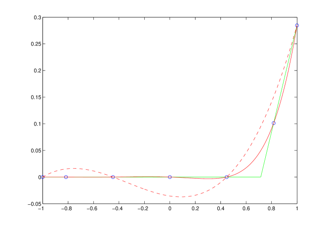
Figure 1: A discontinuous function (solid) and the integrand interpolation using the Gauss-Lobatto rule $Q_{5}[-1,1]$ (dashed) and the Gauss-Kronrod rule $Q_{9}[-1,1]$ (dotted) from Matlab’s quadl integrator. Note that although both quadratures return the same result, the interpolated functions differ significantly.

It is for this reason that instead of trying to compute the error as in Equation (8), we will use the $L_{2}$ norm of the difference between the integrand $f(x)$ and the interpolant $g_{n}(x)$

$$\left[\int_{-1}^{1}\left(g_{n}(x)-f(x)\right)^{2}\,\mbox{d}x\right]^{1/2}.$$ (9)

This is an approximation of the integration error Equation (8). The error estimate will only be zero if the interpolated integrand matches the integrand on the entire interval

$$g_{n}(x)=f(x),\quad x\in[-1,1].$$

In such a case, the integral will also be computed exactly. The error Equation (9) is therefore, assuming we can evaluate it reliably, not susceptible to “accidentally small” values.

Since we do not know $f(x)$ explicitly, i.e. we can only sample $f(x)$ in a point-wise fashion, we cannot evaluate the right-hand side of Equation (9) exactly. In a first, naive approach, we could compute two interpolations $g^{(1)}_{n_{1}}(x)$ and $g^{(2)}_{n_{2}}(x)$ of different degree where $n_{1}<n_{2}$. If we assume, as is done for error estimators using quadrature rules of differing degree, that $g^{(2)}_{n_{2}}(x)$ is a sufficiently precise approximation of the integrand

$$g^{(2)}_{n_{2}}(x)\approx f(x),\quad x\in[-1,1]$$

then we can approximate the error of the interpolation $g^{(1)}_{n_{1}}(x)$ as

$$\left[\int_{-1}^{1}\left(f(x)-g^{(1)}_{n_{1}}(x)\right)^{2}\,\mbox{d}x\right]^{1/2} \approx \left[\int_{-1}^{1}\left(g^{(2)}_{n_{2}}(x)-g^{(1)}_{n_{1}}(x)\right)^{2}\,\mbox{d}x\right]^{1/2}$$

$$= \|\mathbf{c}^{(2)}-\mathbf{c}^{(1)}\|$$

where $\mathbf{c}^{(1)}$ and $\mathbf{c}^{(2)}$ are the vectors of the coefficients of $g^{(1)}_{n_{1}}(x)$ and $g^{(2)}_{n_{2}}(x)$ respectively and $c^{(1)}_{i}=0$ where $i>n_{1}$. Our first, naive error estimate is hence

$$\varepsilon_{\mathsf{naive}}:=\|\mathbf{c}^{(1)}-\mathbf{c}^{(2)}\|.$$ (10)

This error estimate, however, only applies to the lower-degree estimate $g^{(1)}_{n_{1}}(x)$. Yet if we are going to compute the higher-degree estimate $g^{(2)}_{n_{2}}(x)$, it would be preferable to have an error estimate for that approximation.

We can, taking a different approach, use the interpolation error

$$|g_{n}(x)-f(x)|=\left|\frac{f^{(n+1)}(\xi_{x})}{(n+1)!}\pi_{n}(x)\right|,\quad x\in[-1,1]$$ (11)

where $\xi_{x}\in[-1,1]$ depends on the value of $x$ and where $\pi_{n}(x)=\prod_{i=0}^{n}(x-x_{i})$ is the Newton basis polynomial over the nodes of the interpolation $g_{n}(x)$. Taking the $L_{2}$-norm on both sides of Equation (11) we obtain

$$\varepsilon=\left[\int_{-1}^{1}\left(g_{n}(x)-f(x)\right)^{2}\,\mbox{d}x\right]^{1/2}=\left[\int_{-1}^{1}\left(\frac{f^{(n+1)}(\xi_{x})}{(n+1)!}\right)^{2}\pi^{2}_{n}(x)\,\mbox{d}x\right]^{1/2}.$$

Since $\pi_{n}^{2}(x)$ is, by definition, positive for any $x$, we can apply the mean value theorem of integration and extract the derivative resulting in

$$\varepsilon=\left[\int_{-1}^{1}\left(g_{n}(x)-f(x)\right)^{2}\,\mbox{d}x\right]^{1/2}=\left|\frac{f^{(n+1)}(\xi)}{(n+1)!}\right|\left[\int_{-1}^{1}\pi^{2}_{n}(x)\,\mbox{d}x\right]^{1/2},\quad\xi\in[-1,1].$$ (12)

Given two interpolations $g^{(1)}_{n}(x)$ and $g^{(2)}_{n}(x)$ over a non-identical set of nodes, we can compute the interpolation errors

$$\left|g^{(\star)}_{n}(x)-f(x)\right|=\left|\frac{f^{(n+1)}(\xi_{\star})}{(n+1)!}\pi^{(\star)}_{n}(x)\right|,\quad\xi_{\star}\in[-1,1],\quad\star\in\{1,2\}$$ (13)

where $\pi^{(1)}_{n}(x)$ and $\pi^{(2)}_{n}(x)$ are the Newton basis polynomials over the nodes of $g^{(1)}_{n}(x)$ and $g^{(2)}_{n}(x)$ respectively. If we assume that $f^{(n+1)}(x)$ is constant for $x\in[-1,1]$ (a stricter version of the “sufficiently smooth” assumption for the purpose of deriving this error estimate) and take the $L_{2}$-norm of the difference between both errors, we obtain

$$\left[\int_{-1}^{1}\left(g^{(1)}_{n}(x)-g^{(2)}_{n}(x)\right)^{2}\,\mbox{d}x\right]^{1/2}=\left|\frac{f^{(n+1)}(\xi)}{(n+1)!}\right|\left[\int_{-1}^{1}\left(\pi^{(1)}_{n}(x)-\pi^{(2)}_{n}(x)\right)^{2}\,\mbox{d}x\right]^{1/2}.$$ (14)

If we represent the interpolations $g^{(1)}_{n}(x)$ and $g^{(2)}_{n}(x)$ by their coefficients $\mathbf{c}^{(1)}$ and $\mathbf{c}^{(2)}$ respectively, then we can write the left-hand side of Equation (14) as

$$\left\|\mathbf{c}^{(1)}-\mathbf{c}^{(2)}\right\|=\left|\frac{f^{(n+1)}(\xi)}{(n+1)!}\right|\left[\int_{-1}^{1}\left(\pi^{(1)}_{n}(x)-\pi^{(2)}_{n}(x)\right)^{2}\,\mbox{d}x\right]^{1/2}.$$ (15)

Similarly, if we represent the Newton basis polynomials $\pi^{(1)}_{n}(x)$ and $\pi^{(2)}_{n}(x)$ by their coefficients $\mathbf{b}^{(1)}$ and $\mathbf{b}^{(2)}$ respectively

$$\pi^{(1)}_{n}(x)=\sum_{i=0}^{n+1}b^{(1)}_{i}p_{i}(x),\quad\pi^{(2)}_{n}(x)=\sum_{i=0}^{n+1}b^{(2)}_{i}p_{i}(x),$$ (16)

we can isolate the fraction on the right hand side of Equation (15)

$$\left|\frac{f^{(n+1)}(\xi)}{(n+1)!}\right|=\frac{\left\|\mathbf{c}^{(1)}-\mathbf{c}^{(2)}\right\|}{\left\|\mathbf{b}^{(1)}-\mathbf{b}^{(2)}\right\|}.$$ (17)

Inserting this expression into the original error estimate (Equation (12)) for the interpolation $g^{(1)}_{n}(x)$ we then obtain

$$\left[\int_{-1}^{1}\left(g^{(1)}_{n}(x)-f(x)\right)^{2}\,\mbox{d}x\right]^{1/2}=\displaystyle\|\mathbf{b}^{(1)}\|\frac{\left\|\mathbf{c}^{(1)}-\mathbf{c}^{(2)}\right\|}{\left\|\mathbf{b}^{(1)}-\mathbf{b}^{(2)}\right\|}=:\varepsilon^{(1)}\\$$

Hence, using two interpolations of the same degree, we obtain the more refined error estimate

$$\varepsilon_{\mathsf{ref}}:=\frac{\|\mathbf{c}^{(1)}-\mathbf{c}^{(2)}\|}{\|\mathbf{b}^{(1)}-\mathbf{b}^{(2)}\|}\|\mathbf{b}^{(1)}\|$$ (18)

for the interpolation $g^{(1)}_{n}(x)$.

Note that if the nodes of the interpolations $g^{(1)}_{n}(x)$ and $g^{(2)}_{n}(x)$ are fixed, we can pre-compute the scaling $\|\mathbf{b}^{(1)}\|/\|\mathbf{b}^{(1)}-\mathbf{b}^{(2)}\|$.

Instead of explicitly computing two different interpolations over an interval $[a,b]$ to construct the error estimate, we can re-use the interpolation from the previous level of recursion after bisection, the coefficients $\mathbf{c}^{\mathsf{old}}$ of which can be computed using Equation (6). Likewise, we can compute the coefficients $\mathbf{b}^{\mathsf{old}}$ of the Newton basis polynomial over the nodes of the previous level in the same way. However, since $\mathbf{b}^{\mathsf{old}}$ and $\mathbf{b}$ are not in the same interval, we have to scale the coefficients of $\mathbf{b}^{\mathsf{old}}$ by $2^{n+1}$ such that Equation (13) holds. In this way, we only need to compute and store a single matrix $\mathbf{P}^{-1}$ and vector $\mathbf{b}$ for a single stencil of interpolation nodes.

As with the previous error estimators, we have also made an assumption of smoothness regarding the integrand by assuming that $f^{(n+1)}(x)$ is constant for $x\in[-1,1]$ to construct Equation (18). We can’t verify this directly, but we can verify if our computed $|\frac{f^{(n+1)}(\xi)}{(n+1)!}|$ (Equation (17)) actually satisfies Equation (13) for the nodes of the first interpolation by testing if

$$\left|g^{(2)}_{n}(x_{i})-f(x_{i})\right|\leq\vartheta_{1}\left|\frac{f^{(n+1)}(\xi)}{(n+1)!}\right|\left|\pi^{(2)}_{n}(x_{i})\right|$$ (19)

is satisfied for all $i=0\dots n$, where the $x_{i}$ are the nodes of the interpolation $g^{(1)}_{n}(x)$. The value $\vartheta_{1}\geq 1$ is an arbitrary relaxation parameter (for the tests in Section 7 we use $\vartheta_{1}=1.1$). If this condition is violated for any of the $x_{i}$, then we use the naive error estimate in Equation (10).

4 Singularities and Undefined Values

Since most adaptive quadrature algorithms are designed for general-purpose use, they will often be confronted with integrands containing singularities or undefined function values. These can cause problems on two levels:

• The quadrature rule has to be evaluated with a non-numerical value such as a $\mathsf{NaN}$ or $\pm\mathsf{Inf}$,

• The integrand may not be as smooth and continuous as the algorithm might assume.

Such problems arise when integrating functions such as

$$\int_{0}^{h}x^{\alpha}\,\mbox{d}x,\quad\alpha<0$$

which have a singularity at $x=0$, or when computing seemingly innocuous integrals such as

$$\int_{0}^{h}\frac{\sin x}{x}\,\mbox{d}x$$

for which the integrand is undefined at $x=0$, yet has a well-defined limit

$$\lim_{x\rightarrow 0}\frac{\sin x}{x}=1.$$

In both cases problems could be avoided by either shifting the integration domain slightly or by modifying the integrand such as to catch the undefined cases and return a correct numerical result. This would, however, require some prior reflection and intervention by the user, which would defeat the purpose of a general-purpose quadrature algorithm.

Most algorithms deal with singularities by ignoring them, setting the offending value of the integrand to 0 [Davis and Rabinowitz (1984), Section 2.12.7]. Another approach, taken by quad and quadl in Matlab, is to shift the edges of the domain by $\varepsilon_{\mathsf{mach}}$ if a non-numerical value is encountered there and to abort with a warning if a non-numerical value is encountered elsewhere in the interval. Since singularities may exist explicitly at the boundaries (e.g. integration of $x^{\alpha}$, $\alpha<0$ in the range $[0,h]$), the explicit treatment of the boundaries is needed, whereas for arbitrary singularities within the interval, the probability of hitting them exactly is somewhat small.

QUADPACK’s QAG and QAGS algorithms take a similar approach: since the nodes of the Gauss and Gauss-Lobatto quadrature rules used therein do not include the interval boundaries, non-numerical values at the interval boundaries will be implicitly avoided. If the algorithm has the misfortune of encountering such a value inside the interval, it aborts.

Our approach to treating singularities will be somewhat different: instead of setting non-numerical values to 0, we will simply remove that node from our interpolation of the integrand. This can be done rather efficiently by computing the interpolation as shown before using a function value of $f(x_{j})=0$ for the offending $j$th node and then down-dating (as opposed to up-dating) the interpolation, i.e. removing the $j$th node from the interpolation, resulting in an interpolation of degree $n-1$:

$$g_{n-1}(x)=\sum_{i=0}^{n-1}c^{(n-1)}_{i}p_{i}(x)$$

which still interpolates the integrand at the remaining $n$ nodes.

The coefficients $c^{(n-1)}_{i}$ of $g_{n-1}(x)$ can be computed, as described in [Gonnet (2009b)], using

$$c^{(n-1)}_{i}=c_{i}-\frac{c_{n}}{b^{(n-1)}_{n}}b^{(n-1)}_{i},\quad i=0\dots n$$

where the $c_{i}$ are the computed coefficients of $g_{n}(x)$ and the $b^{(n-1)}_{i}$ are the coefficients of the downdated Newton polynomial computed by solving the upper-triangular system of equations

$$\left(\begin{array}[]{ccccc}\alpha_{0}&-(x_{j}+\beta_{1})&\gamma_{2}\\ &\ddots&\ddots&\ddots\\ &&\alpha_{n-2}&-(x_{j}+\beta_{n-1})&\gamma_{n}\\ &&&\alpha_{n-1}&-(x_{j}+\beta_{n})\\ &&&&\alpha_{n}\end{array}\right)\left(\begin{array}[]{c}b^{(n-1)}_{0}\\ b^{(n-1)}_{1}\\ \vdots\\ b^{(n-1)}_{n-1}\end{array}\right)=\left(\begin{array}[]{c}b_{1}\\ b_{2}\\ \vdots\\ b_{n}\end{array}\right)$$

using back-substitution, where the $b_{i}$ are the coefficients of the Newton polynomial over the nodes of the quadrature rule (Equation (16)) and the $\alpha_{i}$, $\beta_{i}$ and $\gamma_{i}$ are the coefficients of the three-term recurrence relation satisfied by the polynomials of the orthogonal basis:

$$\alpha_{k}p_{k+1}(x)=(x+\beta_{k})p_{k}(x)-\gamma_{k}p_{k-1}(x).$$

The modified vectors $\mathbf{c}^{(n-1)}$ and $\mathbf{b}^{(n-1)}$ are then used in the same way as $\mathbf{c}$ and $\mathbf{b}$ respectively for the computation of the integral and of the error estimate.

5 Divergent Integrals

Divergent integrals are integrals which tend to $\pm\infty$ and thus cause most algorithms to either recurse infinitely or return an incorrect finite result. They are usually caught by limiting the recursion depth or the number of function evaluations artificially. Both approaches do not per se attempt to detect divergent behavior, and may therefore cause the algorithm to fail for complicated yet non-divergent integrals.

ref:Ninham1966 studied the approximation error when computing

$$\int_{0}^{h}x^{\alpha}\,\mbox{d}x$$ (20)

using the trapezoidal rule. The integral exists for $\alpha>-1$ and is divergent otherwise. Following his analysis, we compute the refined error estimate described in Section 3 (Equation (18)) for the intervals $[0,h]$ and $[0,h/2]$ using an 11-node Clenshaw-Curtis quadrature rule and removing the singular node at $x=0$ as described above.

We note that as the algorithm recurses to the leftmost interval, the local error estimate as well as the computed integral itself remain constant for $\alpha=-1$ and increase for $\alpha<-1$. In Figure 2 we plot the ratio of the error estimate in the left sub-interval over the error in the entire interval, $\varepsilon[0,h/2]/\varepsilon[0,h]$, over the parameter $\alpha$. For $\alpha=-1$ the ratio is $1$ meaning that the error estimate of the leftmost interval remains constant even after halving the interval. For $\alpha<-1$, for which the integral diverges, the error estimate in the left half-interval is larger than the error estimate over the entire interval.

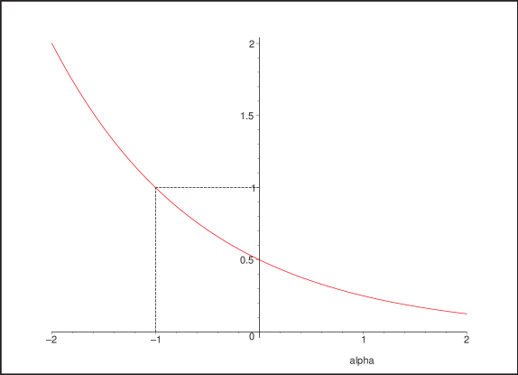
Figure 2: Ratio of the error estimates for $\int_{0}^{h}x^{\alpha}\,\mbox{d}x$ for the intervals $[0,h/2]$ over $[0,h]$ for different $\alpha$. Note that the error grows (ratio $>1$) for $\alpha<-1$, where the integral is divergent.

The rate at which the error decreases (or, in this case, increases) may be a good indicator for the convergence or divergence of the integral in Equation (20), where the singularity is at the edge of the domain, yet it does not work as well for the shifted singularity

$$\int_{0}^{h}|x-\beta|^{\alpha}\,\mbox{d}x,\quad\beta\in[0,h/2].$$ (21)

Depending on the location of the singularity ($x=\beta$), the ratio of the error estimates over $[0,h]$ and $[0,h/2]$ varies widely for both $\alpha>-1$ and $\alpha\leq-1$ and can not be used to determine whether the integral diverges or not. In Figure 3 we have shaded the regions in which the ratio of the error estimates $\varepsilon[0,h/2]/\varepsilon[0,h]>1$ for different values of $\alpha$ and the location of the singularity $\beta$. For this ratio to be a good indicator for the value of $\alpha$ (and hence the convergence/divergence of the integral), the shaded area should at least partially cover the lower half of the plot where $\alpha<-1$, which it does not.

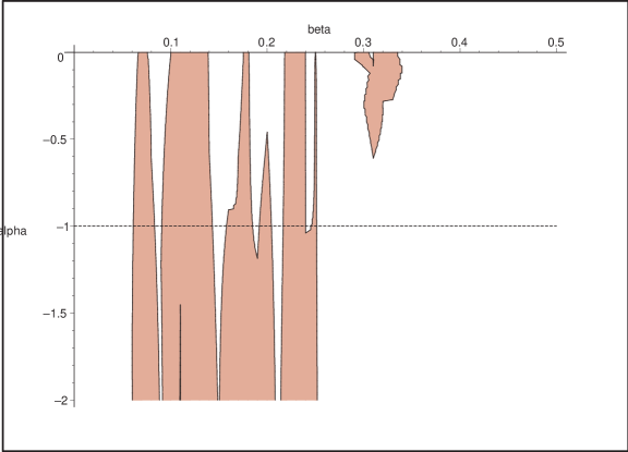
Figure 3: Contour of the ratio of the error estimates for $\int_{0}^{h}|x-\beta|^{\alpha}\,\mbox{d}x$ over the intervals $[0,1]$ and $[0,1/2]$. The filled area represent the region in which this ratio is larger than 1.

A more reliable approach consist of comparing the computed integral in two successive intervals $[a,b]$ and $[a,(a+b)/2]$ or $[(a+b)/2,b]$. For the integrand in Equation (20), the integral in the left sub-interval $[0,h/2]$ is larger than that over the interval $[0,h]$ when $\alpha<-1$. For the integral in Equation (21) the ratio of the integrals in the intervals $[0,h]$ and $[0,h/2]$ is larger than 1 for most cases where $\alpha\leq-1$ (see Figure 4).

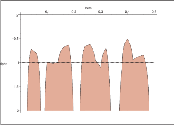
Figure 4: Contour of the ratio of the integral estimates for $\int_{0}^{h}|x-\beta|^{\alpha}\,\mbox{d}x$ over the intervals $[0,1]$ and $[0,1/2]$. The filled area represent the region in which this ratio is larger than 1.

Although this relation (ratio $>1\Rightarrow\alpha<-1$), which is independent of the interval $h$, is not always correct, it can still be used as a statistical hint for the integrand’s behavior during subdivision. In the area $-2\leq\alpha\leq-1$ it is correct approximately two thirds of the time. We will therefore count the number of times that

$$\frac{Q_{n}[a,(a+b)/2]}{Q_{n}[a,b]}\geq 1\quad\mbox{or}\quad\frac{Q_{n}[(a+b)/2,b]}{Q_{n}[a,b]}\geq 1$$ (22)

during subdivision. Note that since the integral goes to either $+\infty$ or $-\infty$, the integral approximations will be of the same sign and thus the sign of the ratios do not matter. If this count exceeds some maximum number and is more than half of the recursion depth – i.e. the ratio of integrals was larger than one over more than half of the subdivisions – then we declare the integral to be divergent and return an error or warning to the user to this effect.

6 The Algorithm

We present the algorithm in two variants, Algorithm 3 and Algorithm 4, using both the naive and the refined error estimates presented in Section 3. Both algorithms follow the globally adaptive general scheme shown in Algorithm 2.

Algorithm 3 int_naive $(f,a,b,\tau)$

1:  for $i=0\dots n_{d_{\mathsf{max}}}$ do $f_{i}\leftarrow f\left((a+b)/2-(a-b)x^{(m)}_{i}/2\right)$ end for (evaluate the integrand at the nodes $x^{(m)}_{i}$)

2:  $\mathbf{c}^{(d_{\mathsf{max}}-1)}\leftarrow(\mathbf{P}^{(d_{\mathsf{max}}-1)})^{-1}\mathbf{f}[1:2:n_{m}+1]$, $\mathbf{c}^{(d_{\mathsf{max}})}\leftarrow(\mathbf{P}^{(d_{\mathsf{max}})})^{-1}\mathbf{f}$ (compute the interpolation coefficients)

3:  $q_{0}\leftarrow(b-a)\boldsymbol{\omega}^{\mathsf{T}}\mathbf{c}^{(d_{\mathsf{max}})}/2$ (approximate the integral as per Equation (5))

4:  $\varepsilon_{0}\leftarrow(b-a)\|\mathbf{c}^{(d_{\mathsf{max}})}-\mathbf{c}^{(d_{\mathsf{max}}-1)}\|/2$ (approximate the error)

5:  $H\leftarrow\{[a,b,\mathbf{c}^{(d_{\mathsf{max}})},q_{0},\varepsilon_{0},d_{\mathsf{max}},0,0]\}$ (init the heap with the first interval)

6:  $\varepsilon_{\mathsf{xs}}\leftarrow 0$, $q_{\mathsf{xs}}\leftarrow 0$ (init the excess error and integral)

7:  while $\sum_{\varepsilon_{i}\in H}\varepsilon_{i}>\tau$ do

8:     $k\leftarrow\arg\max_{k}\varepsilon_{k}$ (get the index of the interval with the largest error)

9:     $m\leftarrow(a_{k}+b_{k})/2$, $h\leftarrow(b_{k}-a_{k})/2$

10:     $\mathsf{split}\leftarrow\mathbf{false}$ (init $\mathsf{split}$)

11:     if $\varepsilon_{k}<|q_{k}|\varepsilon_{\mathsf{mach}}\mbox{cond}(\mathbf{P}^{(d_{k})})\ \vee$ interval too small then

12:        $\varepsilon_{\mathsf{xs}}\leftarrow\varepsilon_{\mathsf{xs}}+\varepsilon_{k}$, $q_{\mathsf{xs}}\leftarrow q_{\mathsf{xs}}+q_{k}$ (collect the excess error and integral)

13:        $H\leftarrow H\setminus\{[a_{k},b_{k},\mathbf{c}^{\mathsf{old}},q_{k},\varepsilon_{k},d_{k},\mathsf{nr}_{\mathsf{div}},\mathsf{nr}_{\mathsf{rec}}]\}$ (remove the $k$th interval)

14:     else if $d_{k}<d_{\mathsf{max}}$ then

15:        $d_{k}\leftarrow d_{k}+1$ (increase the degree in this interval)

16:        for $i=0\dots n_{d_{k}}$ do $f_{i}\leftarrow f\left(m-hx^{(d_{k})}_{i}/2\right)$ end for

17:        $\mathbf{c}^{(d_{k})}=(\mathbf{P}^{(d_{k})})^{-1}\mathbf{f}$ (compute the new interpolation coefficients)

18:        $q_{k}\leftarrow h\boldsymbol{\omega}^{\mathsf{T}}\mathbf{c}^{(d_{k})}$ (approximate the new integral)

19:        $\varepsilon_{k}\leftarrow h\|\mathbf{c}^{(d_{k})}-\mathbf{c}^{\mathsf{old}}\|$ (approximate the new error)

20:        $\mathsf{split}\leftarrow\frac{\|\mathbf{c}^{(d_{k})}-\mathbf{c}^{\mathsf{old}}\|}{\|\mathbf{c}^{(d_{k})}\|}>\mathsf{hint}$ (check change in the coefficients)

21:     else

22:        $\mathsf{split}\leftarrow\mathbf{true}$ (split the interval if we are already at highest-degree rule)

23:     end if

24:     if $\mathsf{split}$ then

25:        $H\leftarrow H\setminus\{[a_{k},b_{k},\mathbf{c}^{\mathsf{old}},q_{k},\varepsilon_{k},d_{k},\mathsf{nr}^{\mathsf{old}}_{\mathsf{div}},\mathsf{nr}_{\mathsf{rec}}]\}$ (remove the $k$th interval)

26:        for $i=0\dots n_{0}$ do

27:           $f^{\mathsf{left}}_{i}\leftarrow f\left((a_{k}+m)/2+hx^{(0)}_{i}/2\right)$, $f^{\mathsf{right}}_{i}\leftarrow f\left((m+b_{k})/2+hx^{(0)}_{i}/2\right)$

28:        end for

29:        for $\mathsf{half}\in\{\mathsf{left},\mathsf{right}\}$ do

30:           $\mathbf{c}^{\mathsf{half}}=(\mathbf{P}^{(0)})^{-1}\mathbf{f}^{\mathsf{half}}$ (compute the new interpolation coefficients)

31:           $q_{\mathsf{half}}\leftarrow hc^{\mathsf{half}}_{0}/\sqrt{2}$ (approximate the new integral)

32:           if $q_{\mathsf{half}}\geq q^{(0)}_{k}$ then $\mathsf{nr}^{\mathsf{half}}_{\mathsf{div}}\leftarrow\mathsf{nr}^{\mathsf{old}}_{\mathsf{div}}+1$ else $\mathsf{nr}^{\mathsf{half}}_{\mathsf{div}}\leftarrow\mathsf{nr}^{\mathsf{old}}_{\mathsf{div}}$ end if

33:           if $\mathsf{nr}^{\mathsf{half}}_{\mathsf{div}}>\mathsf{nr}_{\mathsf{divmax}}\wedge 2\mathsf{nr}^{\mathsf{half}}_{\mathsf{div}}>\mathsf{nr}_{\mathsf{rec}}$ then return error end if (abort on divergence)

34:           $\varepsilon_{\mathsf{half}}\leftarrow h\|\mathbf{c}^{\mathsf{half}}-\mathbf{T}^{\mathsf{half}}\mathbf{c}^{\mathsf{old}}\|$ (approximate the new error)

35:        end for

36:        $H\leftarrow H\cup\{[a_{k},m,\mathbf{c}^{\mathsf{left}},q_{\mathsf{left}},\varepsilon_{\mathsf{left}},0,\mathsf{nr}^{\mathsf{left}}_{\mathsf{div}},\mathsf{nr}_{\mathsf{rec}}+1],$

37:                  $[m,b_{k},\mathbf{c}^{\mathsf{right}},q_{\mathsf{right}},\varepsilon_{\mathsf{right}},0,\mathsf{nr}^{\mathsf{right}}_{\mathsf{div}},\mathsf{nr}_{\mathsf{rec}}+1]\}$ (push the new intervals back on the heap)

38:     end if

39:  end while

40:  return  $\left[q_{\mathsf{xs}}+\sum_{q_{i}\in H}q_{i}\right],\left[\varepsilon_{\mathsf{xs}}+\sum_{\varepsilon_{i}\in H}\varepsilon_{i}\right]$ (return the integral and the error)

The first algorithm (Algorithm 3) uses the naive error estimate in Equation (10) in a doubly adaptive strategy using $d_{\mathsf{max}}+1$ rules of degree $n_{i}=2n_{i-1}$, $i=1\dots d_{\mathsf{max}}$, using the nodes $\mathbf{x}^{(i)}$ and the Vandermonde-like matrices $\mathbf{P}^{(i)}$, $i=0\dots d_{\mathsf{max}}$. For the tests in Section 7, $n_{0}=4$, $\mathsf{hint}=0.1$ and $d_{\mathsf{max}}=3$ were used.

In Lines 1 to 4, the coefficients of the two highest-degree rules are computed and used to approximate the initial integral and error estimate. In Line 5 the heap $H$ is initialized with this interval data. The algorithm then loops until the sum of the errors over all the intervals is below the required tolerance (Line 7). At the top of the loop, the interval with the largest error is selected (Line 8). If the error in this interval is below the numerical accuracy available for the rule used or the interval is too small (i.e. the space between the first two or last two nodes is zero, Line 11), the interval is dropped and its error and integral are accumulated in the excess variables $\varepsilon_{\mathsf{xs}}$ and $q_{\mathsf{xs}}$ (Line 12). If the selected interval has not already used the highest-degree rule (Line 14), the coefficients of the next-higher degree rule are computed and the integral and error estimate are updated (Lines 15 to 19). The interval is bisected if either the highest-degree rule has already been applied or if when increasing the degree of the rule the coefficients change too much (Line 20), analogously to the decision process suggested by ref:Venter2002. For the two new sub-intervals, the coefficients for the lowest-degree rule are computed (Line 30) and used to approximate the integral (Line 31). The number of times the integral increases over the sub-interval is counted in the variables $\mathsf{nr}_{\mathsf{div}}$ (Line 32) and if they exceed $\mathsf{nr}_{\mathsf{divmax}}$ and half of the recursion depth $\mathsf{nr}_{\mathsf{rec}}$ of that interval, the algorithm aborts (Line 33) as per Section 4. Note that since the test in Equation (19) requires that both estimates be of the same degree, we will use, for the estimate $q_{k}^{(0)}$ from the parent interval, the estimate which was computed for the first rule. The error estimate for the new interval is computed by transforming the interpolation coefficients from the parent interval using Equation (6) and using its difference to the interpolation in the new interval (Line 34). When the sum of the errors falls below the required tolerance, the algorithm returns its approximations to the integral and the integration error (Line 40).

Algorithm 4 int_refined $(f,a,b,\tau)$

1:  for $i=0\dots n$ do $f_{i}\leftarrow f\left((a+b)/2-(a-b)x_{i}/2\right)$ end for (evaluate the integrand at the nodes $x_{i}$)

2:  $\mathbf{c}\leftarrow\mathbf{P}^{-1}\mathbf{f}$, (compute the interpolation coefficients)

3:  $q_{0}\leftarrow(b-a)\boldsymbol{\omega}^{\mathsf{T}}\mathbf{c}^{(d_{\mathsf{max}})}/2$ (approximate the integral)

4:  $\varepsilon_{0}\leftarrow\infty$ (start with a somewhat pessimistic appreciation of the error)

5:  $H\leftarrow\{[a,b,\mathbf{c},\mathbf{b},q_{0},\varepsilon_{0},0,0]\}$ (init the heap with the first interval)

6:  $\varepsilon_{\mathsf{xs}}\leftarrow 0$, $q_{\mathsf{xs}}\leftarrow 0$ (init the excess error and integral)

7:  while $\sum_{\varepsilon_{i}\in H}\varepsilon_{i}>\tau$ do

8:     $k\leftarrow\arg\max_{k}\varepsilon_{k}$ (get the index of the interval with the largest error)

9:     $H\leftarrow H\setminus\{[a_{k},b_{k},\mathbf{c}^{\mathsf{old}},\mathbf{b}^{\mathsf{old}},q_{k},\varepsilon_{k},\mathsf{nr}^{\mathsf{old}}_{\mathsf{div}},\mathsf{nr}_{\mathsf{rec}}]\}$ (remove the $k$th interval)

10:     if $\varepsilon_{k}<|q_{k}|\varepsilon_{\mathsf{mach}}\mbox{cond}(\mathbf{P})\ \vee$ interval too small then

11:        $\varepsilon_{\mathsf{xs}}\leftarrow\varepsilon_{\mathsf{xs}}+\varepsilon_{k}$, $q_{\mathsf{xs}}\leftarrow q_{\mathsf{xs}}+q_{k}$ (collect the excess error and integral)

12:     else

13:        $m\leftarrow(a_{k}+b_{k})/2$, $h\leftarrow(b_{k}-a_{k})/2$

14:        for $i=0\dots n$ do

15:           $f^{\mathsf{left}}_{i}\leftarrow f\left((a_{k}+m)/2+hx_{i}/2\right)$, $f^{\mathsf{right}}_{i}\leftarrow f\left((m+b_{k})/2+hx_{i}/2\right)$ (evaluate the integrand at the nodes $x_{i}$ in the sub-intervals)

16:        end for

17:        for $\mathsf{half}\in\{\mathsf{left},\mathsf{right}\}$ do

18:           $\mathbf{c}^{\mathsf{half}}=(\mathbf{P})^{-1}\mathbf{f}^{\mathsf{half}}$ (compute the new interpolation coefficients)

19:           $q_{\mathsf{half}}\leftarrow h\boldsymbol{\omega}^{\mathsf{T}}\mathbf{c}^{\mathsf{half}}$ (approximate the new integral)

20:           if $q_{\mathsf{half}}\geq q_{k}$ then $\mathsf{nr}^{\mathsf{half}}_{\mathsf{div}}\leftarrow\mathsf{nr}^{\mathsf{old}}_{\mathsf{div}}+1$ else $\mathsf{nr}^{\mathsf{half}}_{\mathsf{div}}\leftarrow\mathsf{nr}^{\mathsf{old}}_{\mathsf{div}}$ end if

21:           if $\mathsf{nr}^{\mathsf{half}}_{\mathsf{div}}>\mathsf{nr}_{\mathsf{divmax}}\wedge 2\mathsf{nr}^{\mathsf{half}}_{\mathsf{div}}>\mathsf{nr}_{\mathsf{rec}}$ then return error end if (abort on divergence)

22:           $f^{(n+1)}_{\mathsf{half}}\leftarrow\frac{\|\mathbf{c}^{\mathsf{half}}-\mathbf{T}^{(\mathsf{half})}\mathbf{c}^{\mathsf{old}}\|}{\|\mathbf{b}^{\mathsf{half}}-2^{n+1}\mathbf{T}^{(\mathsf{half})}\mathbf{b}^{\mathsf{old}}\|}$ (approximate the higher derivative)

23:           if $\max\left\{\left|\mathbf{P}\mathbf{c}^{\mathsf{old}}-\mathbf{f}^{\mathsf{half}}\right|-\vartheta_{1}f^{(n+1)}_{\mathsf{half}}\left|\mathbf{P}\mathbf{b}^{\mathsf{old}}\right|\right\}>0$ then

24:              $\varepsilon_{\mathsf{half}}\leftarrow h\|\mathbf{c}^{\mathsf{half}}-\mathbf{c}^{\mathsf{old}}\|$ (compute the un-scaled error)

25:           else

26:              $\varepsilon_{\mathsf{half}}\leftarrow hf^{(n+1)}_{\mathsf{half}}\|\mathbf{b}^{\mathsf{half}}\|$ (compute the extrapolated error)

27:           end if

28:        end for

29:        $H\leftarrow H\cup\{[a_{k},m,\mathbf{c}^{\mathsf{left}},\mathbf{b}^{\mathsf{left}},q_{\mathsf{left}},\varepsilon_{\mathsf{left}},\mathsf{nr}^{\mathsf{left}}_{\mathsf{div}},\mathsf{nr}_{\mathsf{rec}}+1]$, …          $[m,b_{k},\mathbf{c}^{\mathsf{right}},\mathbf{b}^{\mathsf{right}},q_{\mathsf{right}},\varepsilon_{\mathsf{right}},\mathsf{nr}^{\mathsf{left}}_{\mathsf{div}},\mathsf{nr}_{\mathsf{rec}}+1]\}$ (push the new intervals back on the heap)

30:     end if

31:  end while

32:  return  $\left[q_{\mathsf{xs}}+\sum_{q_{i}\in H}q_{i}\right],\left[\varepsilon_{\mathsf{xs}}+\sum_{\varepsilon_{i}\in H}\varepsilon_{i}\right]$ (return the integral and the error)

The second algorithm (Algorithm 4) uses the refined error estimate in Equation (18), which re-uses the coefficients from a previous level of recursion. For the results in Section 7, $n=10$ and $\vartheta_{1}=1.1$ were used.

In Lines 1 to 5 an initial estimate is computed and used to initialize the heap $H$. The error estimate is set to $\infty$ since it can not be estimated (Line 4). While the sum of error estimates is above the required tolerance, the algorithm selects the interval with the largest error estimate (Line 8) and removes it from the heap (Line 9). As with the previous algorithm, if the error estimate is smaller than the numerical precision of the integral or the interval is too small, the interval is dropped (Line 10) and its error and integral estimates are stored in the excess variables $\varepsilon_{\mathsf{xs}}$ and $q_{\mathsf{xs}}$ (Line 11). The algorithm then computes the new coefficients for each sub-interval (Line 18), as well as their integral approximation (Line 19). If the integral over the sub-interval is larger than over the previous interval, the variable $\mathsf{nr}_{\mathsf{div}}$ is increased (Line 20) and if it exceeds $\mathsf{nr}_{\mathsf{divmax}}$ and half of the recursion depth $\mathsf{nr}_{\mathsf{rec}}$, the algorithm aborts with an error (Line 21). In Line 23 the algorithm tests whether the conditions laid out in Equation (19) for the approximation of the $n+1$st derivative hold. If they do not, the un-scaled error estimate is returned (Line 24), otherwise, the scaled estimate is returned (Line 26). Finally, both sub-intervals are returned to the heap (Line 29). Once the required tolerance is met, the algorithm returns its approximations to the integral and the integration error (Line 32).

Although the algorithm descriptions in Algorithms 3 and 4 are quite complete, some details have been omitted for simplicity. First of all, when the function values are computed (Lines 1, 15 and 27 of Algorithm 3 and Lines 1 and 15 of Algorithm 4), it is understood that previously computed function values at the same nodes, i.e. on the edges of the domain for both algorithms or inside the Clenshaw-Curtis rules of increasing degree for Algorithm 3, are re-used and not re-evaluated.

We have also not included the downdate of the interpolations when $\mathsf{NaN}$ or $\pm\mathsf{Inf}$ is encountered. This is done as is shown in Algorithm 5. If, when evaluating the integrand, a non-numerical value is encountered, the function values is set to zero and the index of the node is stored in $\mathsf{nans}$ (Line 4). The coefficients of the interpolation are then computed for those function values (Line 6). For each index in $\mathsf{nans}$, first the coefficients $\mathbf{b}$ of the Newton polynomial over the nodes of the quadrature rule are down-dated as per Equation (4) (Line 8). The downdated $\mathbf{b}$ is then in turn used to downdate the interpolation coefficients $\mathbf{c}$ as per Equation (4) (Line 9).

Furthermore, to improve memory efficiency, both algorithms maintain at most 200 intervals in the heap. If this number is exceeded, the interval with the smallest error estimate is removed and its integral and error estimates are added to the excess variables $q_{\mathsf{xs}}$ and $\varepsilon_{\mathsf{xs}}$ respectively.

Algorithm 5 Interpolation downdate procedure

1:  $\mathsf{nans}\leftarrow\{\}$ (initialize $\mathsf{nans}$)

2:  for $i=0\dots n$ do

3:     $f_{i}\leftarrow f\left(a+\frac{x_{i}+1}{2}(b-a)\right)$ (evaluate the integrand at the nodes $x_{i}$)

4:     if $f_{i}\in\{\mathsf{NaN},\mathsf{Inf}\}$ then $f_{i}\leftarrow 0,\mathsf{nans}\leftarrow\mathsf{nans}\cup\{i\}$ end if (if the result is non-numerical, set the node to zero and remember it)

5:  end for

6:  $\mathbf{c}\leftarrow\mathbf{P}^{-1}\mathbf{f}$ (compute the initial interpolation coefficients)

7:  for $i\in\mathsf{nans}$ do

8:     $\mathbf{b}\leftarrow\mathbf{U}^{-1}_{i}\mathbf{b}$ (downdate the coefficients of the Newton polynomial)

9:     $\mathbf{c}\leftarrow\mathbf{c}-\frac{c_{n}}{b_{n}}\mathbf{b}$ (downdate the coefficients of the interpolation)

10:     $n\leftarrow n-1$ (decrement the degree)

11:  end for

7 Validation

$\tau=10^{-3}$	quadl			DQAGS			da2glob			Algorithm 4			Algorithm 3
$f(x)$	✓	✕	$n_{\mathsf{eval}}$	✓	✕	$n_{\mathsf{eval}}$	✓	✕	$n_{\mathsf{eval}}$	✓	✕	$n_{\mathsf{eval}}$	✓	✕	$n_{\mathsf{eval}}$
Eqn (23)	$395$	$605$	$94.47$	$915$	$85$	$450.62$	$977$	$23$	$95.97$	$1000$	$0$	$361.63$	$1000$	$0$	$281.75$
Eqn (24)	$885$	$115$	$117.48$	$963$	$37$	$399.13$	$1000$	$0$	$59.62$	$1000$	$0$	$306.80$	$1000$	$0$	$175.30$
Eqn (25)	$867$	$133$	$46.14$	$1000$	$0$	$179.13$	$1000$	$0$	$29.14$	$1000$	$0$	$99.39$	$1000$	$0$	$113.36$
Eqn (26)	$360$	$640$	$88.53$	$706$	$294\,(16)$	$409.37$	$882$	$118.5$	$136.50$	$1000$	$0$	$498.56$	$1000$	$0$	$342.02$
Eqn (27)	$265$	$735$	$291.60$	$962$	$38\,(4)$	$1715.74$	$997$	$3$	$480.64$	$1000$	$0$	$1457.63$	$996$	$4$	$990.57$
Eqn (7)	$995$	$5$	$765.39$	$1000$	$0$	$450.53$	$1000$	$0$	$523.35$	$1000$	$0$	$688.98$	$1000$	$0$	$879.37$

$\tau=10^{-6}$	quadl			DQAGS			da2glob			Algorithm 4			Algorithm 3
$f(x)$	✓	✕	$n_{\mathsf{eval}}$	✓	✕	$n_{\mathsf{eval}}$	✓	✕	$n_{\mathsf{eval}}$	✓	✕	$n_{\mathsf{eval}}$	✓	✕	$n_{\mathsf{eval}}$
Eqn (23)	$406$	$594$	$371.64$	$910$	$90$	$1094.27$	$993\,(7)$	$7$	$298.45$	$1000$	$0$	$993.84$	$1000$	$0$	$870.30$
Eqn (24)	$879$	$121$	$237.54$	$906$	$94$	$791.28$	$1000$	$0$	$100.12$	$1000$	$0$	$626.96$	$1000$	$0$	$316.15$
Eqn (25)	$780$	$220$	$103.56$	$987$	$13$	$365.32$	$1000$	$0$	$58.12$	$1000$	$0$	$255.25$	$1000$	$0$	$313.78$
Eqn (26)	$987$	$13$	$482.85$	$931$	$69\,(69)$	$699.22$	$1000$	$0$	$290.52$	$1000$	$0$	$766.88$	$1000$	$0$	$616.96$
Eqn (27)	$994$	$6$	$1318.02$	$999$	$1$	$2075.72$	$1000$	$0$	$870.0$	$1000$	$0$	$2292.21$	$1000$	$0$	$1840.57$
Eqn (7)	$999$	$1$	$2077.80$	$1000$	$0$	$581.41$	$1000\,(1)$	$0$	$695.02$	$1000$	$0$	$1193.97$	$1000$	$0$	$1200.88$

$\tau=10^{-9}$	quadl			DQAGS			da2glob			Algorithm 4			Algorithm 3
$f(x)$	✓	✕	$n_{\mathsf{eval}}$	✓	✕	$n_{\mathsf{eval}}$	✓	✕	$n_{\mathsf{eval}}$	✓	✕	$n_{\mathsf{eval}}$	✓	✕	$n_{\mathsf{eval}}$
Eqn (23)	$360$	$640\,(38)$	$1064.38$	$394\,(389)$	$606\,(597)$	$1525.27$	$874\,(222)$	$126\,(125)$	$627.40$	$897\,(163)$	$103\,(103)$	$2007.81$	$894\,(23)$	$106\,(99)$	$1852.39$
Eqn (24)	$877$	$123$	$357.51$	$609\,(571)$	$391\,(284)$	$1025.39$	$1000$	$0$	$141.82$	$1000$	$0$	$945.20$	$1000$	$0$	$460.87$
Eqn (25)	$779$	$221$	$186.24$	$867\,(734)$	$133\,(98)$	$485.73$	$1000$	$0$	$93.74$	$1000$	$0$	$415.14$	$1000$	$0$	$522.28$
Eqn (26)	$998$	$2$	$1218.57$	$931\,(414)$	$69\,(69)$	$805.81$	$1000$	$0$	$474.81$	$1000$	$0$	$1291.34$	$1000$	$0$	$1078.27$
Eqn (27)	$1000$	$0$	$3375.24$	$999\,(936)$	$1\,(1)$	$2369.30$	$1000$	$0$	$1431.70$	$1000$	$0$	$3915.23$	$1000$	$0$	$3292.26$
Eqn (7)	$945$	$55\,(55)$	$5274.96$	$1000\,(873)$	$0$	$672.17$	$998\,(63)$	$2\,(2)$	$799.86$	$1000\,(3)$	$0$	$2028.08$	$1000\,(1)$	$0$	$1344.78$

$\tau=10^{-12}$	quadl			DQAGS			da2glob			Algorithm 4			Algorithm 3
$f(x)$	✓	✕	$n_{\mathsf{eval}}$	✓	✕	$n_{\mathsf{eval}}$	✓	✕	$n_{\mathsf{eval}}$	✓	✕	$n_{\mathsf{eval}}$	✓	✕	$n_{\mathsf{eval}}$
Eqn (23)	$265$	$735\,(359)$	$2868.37$	$0$	$1000\,(1000)$	$1525.27$	$494\,(267)$	$506\,(506)$	$1068.39$	$558\,(187)$	$442\,(442)$	$9156.03$	$551\,(65)$	$449\,(449)$	$8713.21$
Eqn (24)	$892$	$108$	$489.84$	$3\,(3)$	$997\,(900)$	$1025.39$	$1000$	$0$	$184.42$	$1000\,(2)$	$0$	$1264.45$	$1000$	$0$	$606.67$
Eqn (25)	$781$	$219$	$317.73$	$19\,(15)$	$981\,(949)$	$485.73$	$1000$	$0$	$133.60$	$1000$	$0$	$575.06$	$1000$	$0$	$737.59$
Eqn (26)	$942$	$58$	$3235.86$	$871\,(851)$	$129\,(127)$	$845.92$	$996\,(765)$	$4\,(4)$	$710.62$	$1000\,(592)$	$0$	$10626.40$	$1000\,(428)$	$0$	$17855.83$
Eqn (27)	$711$	$289\,(289)$	$8799.54$	$987\,(987)$	$13\,(13)$	$2400.09$	$1000\,(849)$	$0$	$2068.38$	$1000\,(410)$	$0$	$9619.10$	$1000\,(352)$	$0$	$13596.62$
Eqn (7)	$223$	$777\,(777)$	$9640.14$	$951\,(951)$	$49\,(49)$	$672.17$	$548\,(548)$	$452\,(452)$	$894.86$	$989\,(658)$	$11\,(11)$	$9808.66$	$987\,(514)$	$13\,(13)$	$22433.79$

Table 1: Results of the Lyness-Kaganove tests for $\tau=10^{-3},10^{-6},10^{-9}$ and $10^{-12}$. The columns marked with ✓ and ✕ indicate the number of correct and incorrect results respectively, out of 1 000 runs. The numbers in brackets indicate the number of runs in which a warning was issued. The column $n_{\mathsf{eval}}$ contains the average number of function evaluations required for each run.

In the following, we will test both algorithms described in Section 6 against the following routines:

• quadl, MATLAB’s adaptive quadrature routine [The Mathworks (2003)], based on Gander and Gautschi’s adaptlob [Gander and Gautschi (2001)]. This algorithm uses a 4-point Gauss-Lobatto quadrature rule and its 7-point Kronrod extension.

• DQAGS, QUADPACK’s [Piessens et al. (1983)] adaptive quadrature routine using a 10-point Gauss quadrature rule and its 21-point Kronrod extension as well as the $\varepsilon$-Algorithm to extrapolate the integral and error estimate. The routine is called through the GNU Octave [Eaton (2002)] package’s quad routine.

• da2glob from ref:Espelid2007, which uses a doubly-adaptive strategy over rules of degree 5, 9, 17 and 27 over 5, 9, 17 and 33 equidistant nodes respectively, using the error estimator described in ref:Berntsen1991.

The two algorithms in Section 6 were implemented in the MATLAB programming language.

Over the years, several authors have specified sets of test functions to evaluate the performance and reliability of quadrature routines. In the following, we will use, with some minor modifications, the test “families” suggested by ref:Lyness1977 and the “battery” of functions compiled by ref:Gander1998, which are an extension of the set proposed by ref:Kahaner1971.

The function families used for the Lyness-Kaganove test are

$$\int_{0}^{1}|x-\lambda|^{\alpha}\,\mbox{d}x,\quad \lambda\in[0,1],\ \alpha\in[-0.5,0]$$ (23)

$$\int_{0}^{1}(x>\lambda)e^{\alpha x}\,\mbox{d}x,\quad \lambda\in[0,1],\ \alpha\in[0,1]$$ (24)

$$\int_{0}^{1}\exp(-\alpha|x-\lambda|)\,\mbox{d}x,\quad \lambda\in[0,1],\ \alpha\in[0,4]$$ (25)

$$\int_{1}^{2}10^{\alpha}/((x-\lambda)^{2}+10^{\alpha})\,\mbox{d}x,\quad \lambda\in[1,2],\alpha\in[-6,-3]$$ (26)

$$\int_{1}^{2}\sum_{i=1}^{4}10^{\alpha}/((x-\lambda_{i})^{2}+10^{\alpha})\,\mbox{d}x,\quad \lambda_{i}\in[1,2],\alpha\in[-5,-3]$$ (27)

$$\int_{0}^{1}2\beta(x-\lambda)\cos(\beta(x-\lambda)^{2})\,\mbox{d}x,\quad \lambda\in[0,1],\ \alpha\in[1.8,2],$$

$$\beta=10^{\alpha}/\max\{\lambda^{2},(1-\lambda)^{2}\}$$

where the boolean expressions are evaluated to 0 or 1. The integrals are computed to relative precisions of $\tau=10^{-3}$, $10^{-6}$, $10^{-9}$ and $10^{-12}$ for $1\,000$ realizations of the random parameters $\lambda$ and $\alpha$. The results of these tests are shown in Table 1. For each function, the number of correct and incorrect integrations is given with, in brackets, the number of cases each where a warning (either explicit or whenever an error estimate larger than the requested tolerance is returned) was issued. We consider an integration to be correct only when the returned value is within the required tolerance of the exact result.

The functions used for the “battery” test are

$$\begin{array}[]{rclrcl}f_{1}&=&\textstyle\int_{0}^{1}e^{x}\,\mbox{d}x&f_{14}&=&\textstyle\int_{0}^{10}\sqrt{50}e^{-50\pi x^{2}}\,\mbox{d}x\\ f_{2}&=&\textstyle\int_{0}^{1}(x>0.3)\,\mbox{d}x&f_{15}&=&\textstyle\int_{0}^{10}25e^{-25x}\,\mbox{d}x\\ f_{3}&=&\textstyle\int_{0}^{1}x^{1/2}\,\mbox{d}x&f_{16}&=&\textstyle\int_{0}^{10}50(\pi(2500x^{2}+1))^{-1}\,\mbox{d}x\\ f_{4}&=&\textstyle\int_{-1}^{1}(\frac{23}{25}\cosh(x)-\cos(x))\,\mbox{d}x&f_{17}&=&\textstyle\int_{0}^{1}50(\sin(50\pi x)/(50\pi x))^{2}\,\mbox{d}x\\ f_{5}&=&\textstyle\int_{-1}^{1}(x^{4}+x^{2}+0.9)^{-1}\,\mbox{d}x&f_{18}&=&\textstyle\int_{0}^{\pi}\cos(\cos(x)+3\sin(x)+2\cos(2x)+3\cos(3x))\,\mbox{d}x\\ f_{6}&=&\textstyle\int_{0}^{1}x^{3/2}\,\mbox{d}x&f_{19}&=&\textstyle\int_{0}^{1}\log(x)\,\mbox{d}x\\ f_{7}&=&\textstyle\int_{0}^{1}x^{-1/2}\,\mbox{d}x&f_{20}&=&\textstyle\int_{-1}^{1}(1.005+x^{2})^{-1}\,\mbox{d}x\\ f_{8}&=&\textstyle\int_{0}^{1}(1+x^{4})^{-1}\,\mbox{d}x&f_{21}&=&\textstyle\int_{0}^{1}\sum_{i=1}^{3}\left[\cosh(20^{i}(x-2i/10))\right]^{-1}\,\mbox{d}x\\ f_{9}&=&\textstyle\int_{0}^{1}2(2+\sin(10\pi x))^{-1}\,\mbox{d}x&f_{22}&=&\textstyle\int_{0}^{1}4\pi^{2}x\sin(20\pi x)\cos(2\pi x)\,\mbox{d}x\\ f_{10}&=&\textstyle\int_{0}^{1}(1+x)^{-1}\,\mbox{d}x&f_{23}&=&\textstyle\int_{0}^{1}(1+(230x-30)^{2})^{-1}\,\mbox{d}x\\ f_{11}&=&\textstyle\int_{0}^{1}(1+e^{x})^{-1}\,\mbox{d}x&f_{24}&=&\textstyle\int_{0}^{3}\lfloor e^{x}\rfloor\,\mbox{d}x\\ f_{12}&=&\textstyle\int_{0}^{1}x(e^{x}-1)^{-1}\,\mbox{d}x&f_{25}&=&\textstyle\int_{0}^{5}(x+1)(x<1)+(3-x)(1\leq x\leq 3)\\ f_{13}&=&\textstyle\int_{0}^{1}\sin(100\pi x)/(\pi x)\,\mbox{d}x&&&\quad+2(x>3)\,\mbox{d}x\\ \end{array}$$

where the boolean expressions in $f_{2}$ and $f_{25}$ evaluate to 0 or 1. The functions are taken from ref:Gander1998 with the following modifications:

• No special treatment is given to the case $x=0$ in $f_{12}$, allowing the integrand to return $\mathsf{NaN}$.

• $f_{13}$ and $f_{17}$ are integrated from 0 to 1 as opposed to 0.1 to 1 and 0.01 to 1 respectively, allowing the integrand to return $\mathsf{NaN}$ for $x=0$.

• No special treatment of $x<10^{-15}$ in $f_{19}$ allowing the integrand to return $-\mathsf{Inf}$.

• $f_{24}$ was suggested by J. Waldvogel as a simple yet tricky test function with multiple discontinuities.

• $f_{25}$ was introduced in ref:Gander1998, yet not used in the battery test therein.

The rationale for the modifications of $f_{12}$, $f_{13}$, $f_{17}$ and $f_{19}$ is that we can’t, on one hand, assume that the user was careful enough or knew enough about his or her integrand to remove the non-numerical values, and on the other hand assume that he or she would still resort to a general-purpose quadrature routine to integrate it. Any general purpose quadrature routine should be robust enough to deal with any function, provided by either careful or careless users.

These changes have little effect on quadl and DQAGS since, as mentioned in Section 4, the former shifts the integration boundaries by $\varepsilon_{\mathsf{mach}}$ if a non-numerical value is encountered on the edges of the integration domain and the later uses Gauss and Gauss-Kronrod quadrature rules which do not contain the end-points and thus avoid the $\mathsf{NaN}$ returned at $x=0$ for $f_{12}$, $f_{13}$ and $f_{17}$ and the $\mathsf{Inf}$ at $x=0$ in $f_{19}$. da2glob treats $\mathsf{NaN}$s by setting the offending function values to 1. Due to the rather fortunate coincidence that $f_{12}$, $f_{13}$ and $f_{17}$ all have a limit of 1 for $x\rightarrow 0$, this integrator is in no way troubled by these integrands.

	$\tau=10^{-3}$					$\tau=10^{-6}$					$\tau=10^{-9}$					$\tau=10^{-12}$
$f(x)$	quadl	DQAGS	da2glob	Alg. 4	Alg. 3	quadl	DQAGS	da2glob	Alg. 4	Alg. 3	quadl	DQAGS	da2glob	Alg. 4	Alg. 3	quadl	DQAGS	da2glob	Alg. 4	Alg. 3
$f_{1}$	18	21	9	27	33	18	21	9	27	33	18	21	9	27	33	18	21	17	27	33
$f_{2}$	108	357	61	283	161	198	357	101	603	301	318	357	141	923	441	408	357	181	1243	581
$f_{3}$	48	105	25	107	101	108	231	65	315	429	258	231	137	523	799	618	231	241	827	1191
$f_{4}$	18	21	9	27	33	18	21	9	27	33	18	21	25	27	33	48	21	33	27	33
$f_{5}$	18	21	17	27	33	48	21	33	59	95	48	63	65	59	95	168	63	65	123	219
$f_{6}$	18	21	9	27	33	48	105	41	123	159	108	189	73	251	359	288	189	137	427	607
$f_{7}$	289	231	121	411	269	439	231	285	1035	709	889	231	581	1867	1409	2429	231	965	3291	2179
$f_{8}$	18	21	17	27	33	18	21	25	43	33	48	21	33	59	95	138	63	49	123	95
$f_{9}$	198	315	121	251	261	468	399	233	411	587	1038	567	401	891	991	2808	735	577	1387	1425
$f_{10}$	18	21	9	27	33	18	21	17	27	33	48	21	17	59	33	48	21	33	75	33
$f_{11}$	18	21	9	27	33	18	21	9	27	33	18	21	9	27	33	48	21	17	43	33
$f_{12}$	19	21	9	59	47	19	21	9	59	55	19	21	9	59	63	19	21	9	59	63
$f_{13}$	589	651	929	907	1403	1519	1323	1469	1643	2347	4879	1323	1913	2955	2459	10039	1323	2233	5035	2521
$f_{14}$	78	231	45	187	151	138	231	65	203	183	228	273	105	315	225	588	273	153	379	369
$f_{15}$	78	147	41	187	135	168	189	69	219	159	288	189	101	283	191	708	231	145	379	277
$f_{16}$	18	21	9	27	33	18	21	9	27	33	18	21	9	27	33	18	21	9	27	33
$f_{17}$	79	483	325	619	903	949	777	1065	1195	1491	2839	1323	1725	2123	2419	6469	1323	2077	3419	2451
$f_{18}$	108	105	73	123	145	228	147	129	187	209	738	189	185	379	395	1758	273	273	731	581
$f_{19}$	109	231	65	155	255	229	231	145	475	717	499	231	285	875	1323	1369	231	449	1563	1943
$f_{20}$	18	21	17	27	33	48	21	33	59	33	48	63	65	91	95	168	63	65	187	219
$f_{21}$	138	273	85	235	203	348	357	185	347	391	1158	441	273	1179	653	2748	525	649	1771	1839
$f_{22}$	228	147	241	235	371	888	315	305	379	627	2508	315	385	699	627	5568	315	513	1291	627
$f_{23}$	108	273	93	299	191	258	399	161	411	365	588	441	241	699	569	1608	483	401	1083	957
$f_{24}$	138	1911	453	3227	4515	1878	8211	857	9163	11433	3738	12285	1301	15275	18503	5538	16359	1745	21147	25191
$f_{25}$	108	567	81	379	277	348	819	149	859	593	528	819	201	1339	933	678	819	269	1803	1253

Table 2: Results of battery test for $\tau=10^{-3},10^{-6},10^{-9}$ and $10^{-12}$. The columns contain the number of function evaluations required by each integrator for each tolerance. For each test and tolerance, the best result (least function evaluations) is in bold and unsuccessful runs are stricken through.

The battery functions were integrated for the relative tolerances $\tau=10^{-3}$, $10^{-6}$, $10^{-9}$ and $10^{-12}$ and compared to the exact result, computed analytically. The results are summarized in Table 2, where the number of required function evaluations for each combination of integrand, integrator and tolerance are given. If integration was unsuccessful, the number is stricken through. If the number of evaluations was the lowest for the given integrand and tolerance, it is shown in bold face.

Finally, the integrators were tested on the problem

$$\int_{0}^{1}\left|x-\lambda\right|^{\alpha}\,\mbox{d}x,\quad\lambda\in[0,1]$$

for $1\,000$ realizations of the random parameter $\lambda$ and different values of $\alpha\in[-0.1,-2]$ for a relative tolerance $\tau=10^{-3}$. Since for $\alpha\leq-1$, the integral diverges and can not be computed numerically, we are interested in the warnings or errors returned by the different quadrature routines. The results are shown in Table 3 and Figure 5. For each integrator we give the number of successes and failures as well as, in brackets, the number of times each possible error or warning was returned. The different errors, for each integrator, are:

• quadl: $(\mathsf{Min}/\mathsf{Max}/\mathsf{Inf})$

  • $\mathsf{Min}$: Minimum step size reached; singularity possible.

  • $\mathsf{Max}$: Maximum function count exceeded; singularity likely.

  • $\mathsf{Inf}$: Infinite or Not-a-Number function value encountered.

• DQAGS: $(\mathsf{ier}_{1}/\mathsf{ier}_{2}/\mathsf{ier}_{3}/\mathsf{ier}_{4}/\mathsf{ier}_{5})$

  • $\mathsf{ier}_{1}$: Maximum number of subdivisions allowed has been achieved.

  • $\mathsf{ier}_{2}$: The occurrence of roundoff error was detected, preventing the requested tolerance from being achieved. The error may be under-estimated.

  • $\mathsf{ier}_{3}$: Extremely bad integrand behavior somewhere in the interval.

  • $\mathsf{ier}_{4}$: The algorithm won’t converge due to roundoff error detected in the extrapolation table. It is presumed that the requested tolerance cannot be achieved, and that the returned result is the best which can be obtained.

  • $\mathsf{ier}_{5}$: The integral is probably divergent or slowly convergent.

• da2glob: $(\mathsf{noise}/\mathsf{min}/\mathsf{max}/\mathsf{sing})$

  • $\mathsf{noise}$: The requested tolerance is below the noise level of the problem. Required tolerance may not be met.

  • $\mathsf{min}$: Interval too small. Required tolerance may not be met.

  • $\mathsf{max}$: Maximum number of function evaluations. Required tolerance may not be met.

  • $\mathsf{sing}$: Singularity probably detected. Required tolerance may not be met.

• Algorithms 3 and 4: $(\mathsf{err}/\mathsf{div})$

  • $\mathsf{err}$: The final error estimate is larger than the required tolerance.

  • $\mathsf{div}$: The integral is divergent.

Thus, the results for DQAGS at $\alpha=-0.8$ should be read as the algorithm returning 146 correct and 854 false (requested tolerance not satisfied) results and having returned the error $\mathsf{ier}_{3}$ (bad integrand behavior) 58 times and the error $\mathsf{ier}_{5}$ (probably divergent integral) 4 times.

$\alpha$	quadl	DQAGS	da2glob	Algorithm 4	Algorithm 3
$\alpha=-0.1$	487 / 513 (0/0/0)	979 / 21 (0/0/0/0/0)	979 / 21 (0/0/0/0)	1000 / 0 (0/0)	1000 / 0 (0/0)
$\alpha=-0.2$	459 / 541 (0/0/0)	953 / 47 (0/0/0/0/0)	980 / 20 (0/0/0/0)	1000 / 0 (0/0)	1000 / 0 (0/0)
$\alpha=-0.3$	388 / 612 (0/0/0)	909 / 91 (0/0/0/0/0)	988 / 12 (0/0/0/0)	1000 / 0 (0/0)	1000 / 0 (0/0)
$\alpha=-0.4$	298 / 702 (0/0/0)	852 / 148 (0/0/0/0/0)	985 / 15 (0/0/0/0)	1000 / 0 (0/0)	1000 / 0 (0/0)
$\alpha=-0.5$	181 / 819 (0/0/0)	788 / 212 (0/0/0/0/1)	975 / 25 (0/0/0/0)	1000 / 0 (0/0)	1000 / 0 (0/0)
$\alpha=-0.6$	107 / 893 (0/0/0)	642 / 358 (0/0/0/0/2)	976 / 24 (0/0/0/0)	1000 / 0 (0/0)	1000 / 0 (0/0)
$\alpha=-0.7$	46 / 954 (0/0/0)	451 / 549 (0/0/0/0/1)	958 / 42 (0/84/0/6)	1000 / 0 (0/0)	1000 / 0 (0/0)
$\alpha=-0.8$	4 / 996 (0/0/0)	146 / 854 (0/0/58/0/4)	957 / 43 (0/865/0/0)	998 / 2 (836/0)	970 / 30 (0/3)
$\alpha=-0.9$	0 / 1000 (0/0/98)	3 / 997 (0/0/611/0/18)	0 / 1000 (0/1000/0/0)	0 / 1000 (916/62)	0 / 1000 (918/82)
$\alpha=-1.0$	0 / 1000 (4/0/968)	0 / 1000 (0/0/716/20/119)	0 / 1000 (0/1000/0/0)	0 / 1000 (198/802)	0 / 1000 (431/569)
$\alpha=-1.1$	0 / 1000 (1/0/994)	0 / 1000 (0/0/397/36/482)	0 / 1000 (0/1000/0/0)	0 / 1000 (5/995)	0 / 1000 (40/960)
$\alpha=-1.2$	0 / 1000 (1/0/998)	0 / 1000 (0/0/21/68/897)	0 / 1000 (0/1000/0/0)	0 / 1000 (1/999)	0 / 1000 (6/994)
$\alpha=-1.3$	0 / 1000 (1/0/999)	0 / 1000 (0/0/0/91/908)	0 / 1000 (0/1000/0/0)	0 / 1000 (0/1000)	0 / 1000 (6/994)
$\alpha=-1.4$	0 / 1000 (0/588/412)	0 / 1000 (0/0/0/117/883)	0 / 1000 (0/1000/0/0)	0 / 1000 (0/1000)	0 / 1000 (5/995)
$\alpha=-1.5$	0 / 1000 (0/986/14)	0 / 1000 (0/0/0/191/809)	0 / 1000 (0/998/2/0)	0 / 1000 (0/1000)	0 / 1000 (5/995)
$\alpha=-1.6$	0 / 1000 (0/999/1)	0 / 1000 (0/0/0/254/746)	0 / 1000 (0/994/6/0)	0 / 1000 (0/1000)	0 / 1000 (4/996)
$\alpha=-1.7$	0 / 1000 (0/1000/0)	0 / 1000 (0/0/0/315/685)	0 / 1000 (0/995/5/0)	0 / 1000 (0/1000)	0 / 1000 (4/996)
$\alpha=-1.8$	0 / 1000 (0/1000/0)	0 / 1000 (0/0/0/348/652)	0 / 1000 (0/990/10/0)	0 / 1000 (0/1000)	0 / 1000 (4/996)
$\alpha=-1.9$	0 / 1000 (0/1000/0)	0 / 1000 (0/0/1/387/612)	0 / 1000 (0/981/19/0)	0 / 1000 (0/1000)	0 / 1000 (3/997)
$\alpha=-2.0$	0 / 1000 (0/1000/0)	0 / 1000 (0/0/0/433/567)	0 / 1000 (0/985/15/0)	0 / 1000 (0/1000)	0 / 1000 (3/997)

Table 3: Results of computing $\int_{0}^{1}\left|x-\lambda\right|^{\alpha}\,\mbox{d}x$ for $1\,000$ realizations of $\lambda\in[0,1]$ for different $\alpha$. The columns contain the number of correct/incorrect integrations as well as the number of times (in brackets) the different errors or warnings of each algorithm were returned. Thus, the results for DQAGS at $\alpha=-0.8$ should be read as the algorithm returning 146 correct and 854 false results and having returned the error $\mathsf{ier}_{3}$ 58 times and the error $\mathsf{ier}_{5}$ 4 times.

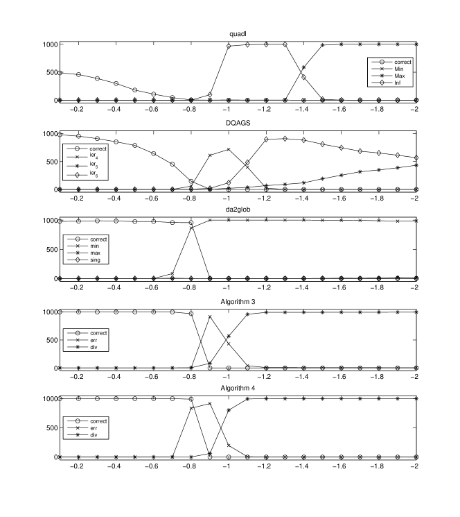
Figure 5: Results of computing $\int_{0}^{1}\left|x-\lambda\right|^{\alpha}\,\mbox{d}x$ for $1\,000$ realizations of $\lambda\in[0,1]$ for different values of $\alpha$ ($x$-axis). The curves represent the number of correct integrations and the number of times each different warning was issued for each value of $\alpha$.

8 Discussion

As can be seen from the results in Table 1, for the integrands in the Lyness-Kaganove test, both new algorithms presented in Section 6 are clearly more reliable than quadl and DQAGS. MATLAB’s quadl performs best for high precision requirements (small tolerances, best results for $\tau=10^{-9}$), yet still fails often without warning. QUADPACK’s DQAGS does better for low precision requirements (large tolerances, best results for $\tau=10^{-3}$), yet also fails often, more often than not with a warning.

Espelid’s da2glob does significantly better, with only a few failures at $\tau=10^{-3}$ (without warning) and a large number of failures for Equation (7) at $\tau=10^{-12}$, albeit all of them with prior warning. The former are due to the error estimate not detecting specific features of the integrand due to the interpolating polynomial looking smooth, when it is, in fact, singular (see Figure 7). The latter were due to the integral estimates being affected by noise (most often in the 17-point rule), which was, in all cases, detected and warned against by the algorithm.

The new algorithms fail only for Equation (23) at small tolerances since the integral becomes numerically impossible to evaluate (there are not sufficient machine numbers near the singularity to properly resolve the integrand), for which a warning is issued. This problem is shared by the other integrators as well. Algorithm 3 also fails a few times when integrating Equation (27). In all such cases, one of the peaks was missed completely by the lower-degree rules, giving the appearance of a flat curve. Both algorithms also failed a few times on Equation (7) in cases where the resulting integral was several orders of magnitude smaller than the function values themselves, making the required tolerance practically un-attainable.

Whereas the new algorithms out-perform the others in terms of reliability, they do so at a cost of a higher number of function evaluations. On average, Algorithm 3 uses about twice as many function evaluations as da2glob, whereas Algorithm 4 uses roughly six times as many.

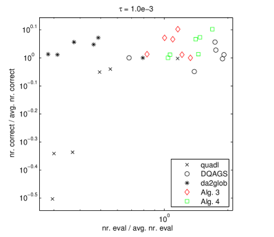
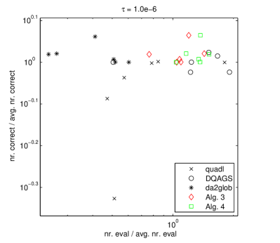
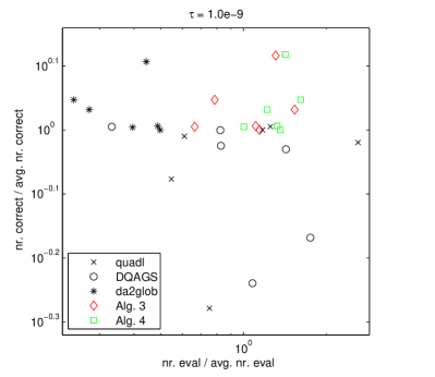
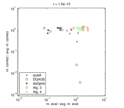
Figure 6: Scatter-plots of the results of the Lyness-Kaganove test-suite for each tolerance. Each point represents one of the test functions (Equations 23 to 7). Its location is determined by the relative number of function evaluations (on the $x$-axis) and the relative number of correct evaluations (on the $y$-axis).

The results are summarized in Figure 6. The plots, for each tolerance and integrand, show where each algorithm stand in terms of relative reliability and relative efficiency. If we divide the plots into four regions

we can see that whereas da2glob is clearly efficient and reliable, the two new algorithms are slightly more reliable, yet slow. The results for quadl and QUADPACK’s DQAGS are scattered over all four regions.

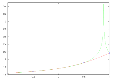
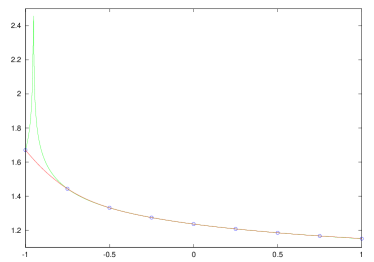
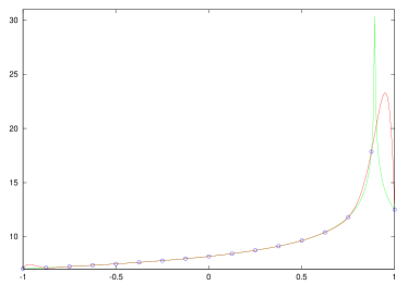
Figure 7: Some cases in which the 5, 9 and 17-point rules used in da2glob fail to detect a singularity (as in Equation (23)). The assumed integrand (red) is sufficiently smooth such that its higher-degree coefficients, from which the error estimate is computed, are near zero.

This trend is also visible in the results of the “battery” test (Table 2). Algorithms 3 and 4 fail on $f_{21}$ for all but the highest and second-highest tolerances respectively, since the third peak at $x=0.6$ is missed completely. da2glob also does quite well, failing on $f_{21}$ at the same tolerances and for the same reasons as the new algorithms and on $f_{24}$ for $\tau<10^{-3}$, using, however, in almost all cases, less function evaluations than Algorithms 3 or 4.

It is interesting to note that quadl, DAQGS and da2glob all failed to integrate $f_{24}$ for tolerances $\tau<10^{-3}$. A closer look at the intervals that caused each algorithm to fail (see Figure 8) reveals that in all cases, multiple discontinuities in the same interval caused the error estimate to be accidentally small, leading the algorithms to erroneously assume convergence. This is not a particularity of the interval chosen: if we integrate

$$\int_{0}^{\lambda}\lfloor e^{x}\rfloor\,\mbox{d}x,\quad\lambda\in[2.5,3.5]$$ (29)

for $1\,000$ realizations of the random parameter $\lambda$ for $\tau=10^{-6}$ using these three integrators, they fail on $894$, $945$ and $816$ of the cases respectively. Both Algorithms 3 and 4 succeed in all cases.

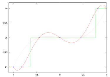
a  b  c 

Figure 8: Intervals in which the error estimates of quadl (a), DQAGS (b) and da2glob (c) failed for $f_{24}$. The interpolatory polynomials used to compute the error estimates are shown in red.

One could argue that the different error estimates are all equally good and the different ratios of reliability vs. efficiency are only due to their parameterization, i.e. their scaling of the error estimate. We can test this hypothesis by scaling the error estimates of all five algorithms by the smallest value $\rho$ such that the 1 000 runs at $\tau=10^{-3}$ for Equation (23) produce no incorrect results:

$\tau=10^{-3}$	quadl		DQAGS		da2glob		Algorithm 4		Algorithm 3
$f(x)$	$\rho$	$n_{\mathsf{eval}}$	$\rho$	$n_{\mathsf{eval}}$	$\rho$	$n_{\mathsf{eval}}$	$\rho$	$n_{\mathsf{eval}}$	$\rho$	$n_{\mathsf{eval}}$
Eqn (23)	40 000	783.18	—	—	50	229.40	0.006	319.24	0.02	243.85

For quadl, a scaling of $\rho=40\,000$ was necessary, resulting in an 8-fold increase in the number of required evaluations and for QUADPACK’s DQAGS, no amount of scaling produced the correct result. For da2glob, Algorithm 3 and Algorithm 4, only moderate scaling was necessary, bringing the number of required function evaluations much closer to each other. There is, therefore, for da2glob a potential for tuning empirical scaling factors towards more reliability, yet at the cost of close to the same number of function evaluations as Algorithms 3 and 4, at least for Equation (23).

This approach, however, breaks down completely for Equation (29). As can be seen in Figure 8, the error estimates which cause the individual algorithms to fail are not merely small: they are zero, and hence no amount of scaling will fix them. The two new algorithms are therefore not only more reliable due to a stricter (or more pessimistic) scaling of the error estimate, but mainly due to the fundamentally different type of error estimate, which is less prone to accidentally small estimates (see [Gonnet (2009a)]).

In the final test evaluating divergent integrals (Table 3), quadl fails to distinguish between divergent and non-divergent integrals, reporting that a non-numerical value was encountered for $-1.0\geq\alpha\geq-1.4$ and then aborting after the maximum $10\,000$ function evaluations for $\alpha<1.4$. For $\alpha<-1.0$, DQAGS reports the integral to be either subject to too much rounding error or divergent. The latter correct result was returned in more than half of the cases tested. In most cases where $\alpha<-0.8$, da2glob aborted, reporting that the smallest interval size had been reached, or, in some cases, that the maximum number of evaluations (by default $10\,000$) had been exceeded. All these cases were accompanied by an additional warning that a singularity had probably been detected. For $\alpha=-0.8$, Algorithm 4 fails with a warning that the required tolerance was not met and as of $\alpha<-1.1$ both Algorithms 4 and 3 abort, correctly, after deciding that the integral is divergent.

We conclude that the new Algorithms 4 and 3, presented herein, are more reliable than MATLAB’s quadl, QUADPACK’s DQAGS and Espelid’s da2glob. This higher reliability is not due to a stricter scaling of the error, but to a new type of error estimator which avoids most of the problems observed in the other algorithms. This increased reliability comes at a cost of two to six times higher number of function evaluations required for complicated integrands such as those in Equations 23 to 7.

The tradeoff between reliability and efficiency should, however, be of little concern in the context of automatic or general-purpose quadrature routines, which should work reliably for any type of integrand. Most modifications which increase efficiency usually rely on making certain assumptions on the integrand, e.g. smoothness, continuity, non-singularity, monotonically decaying coefficients, etc… If, however, the user knows enough about his or her integrand as to know that these assumptions are indeed valid and therefore that the algorithm will not fail, then he or she knows enough about the integrand as to not have to use a general-purpose quadrature routine and, if efficiency is crucial, should consider integrating it by a specialized routine or even trying to do so analytically.

In making any assumptions for the user, we would be making two mistakes:

1. The increase in efficiency would reward users who, despite knowing enough about their integrand to trust the quadrature rule, have not made the effort to look for a specialized or less general routine,

2. The decrease in reliability punishes users who have turned to a general-purpose quadrature routine because they knowingly can not make any assumptions regarding their integrand.

It is for this reason that we should have no qualms whatsoever in sacrificing a bit of efficiency on some special integrands for much more reliability on tricky integrands for which we know, and can therefore assume, nothing.

Ideally, software packages such as Matlab or libraries such as the Gnu Scientific Library [Galassi et al. (2009)] should offer both heavy-duty quadrature routines such as Algorithms 3 and 4 presented herein, alongside other efficient routines, such as da2glob [Espelid (2007)] for less tricky integrands, as well as even more efficient methods (e.g. the exponentially convergent integrator proposed by ref:Waldvogel2009) for analytic (continuous and smooth) integrands, allowing the user to choose according to his or her specific needs or level of understanding regarding the integrand.

9 Acknowledgements

I would like to thank Walter Gander who supervised my PhD thesis which resulted in this work. Further thanks go to Jörg Waldvogel, François Cellier, Gradimir Milovanović, Aleksandar Cvetković, Marija Stanić, Geno Nikolov and Borislav Bojanov who, through their collaboration in the Swiss National Science Foundation (SNSF) SCOPES Project (Nr. IB7320-111079/1, 2005–2008) “New Methods for Quadrature”, provided not only valuable answers, but also the right questions, as well as to Gaston Gonnet for his input on several topics regarding the algorithms and the manuscript itself. Finally, I would like to thank the anonymous reviewers who’s corrections and suggestions, especially those regarding the graphical representation of the results, made this a better manuscript.

..

References

- Bauer et al. (1963) Bauer, F. L., Rutishauser, H., and Stiefel, E. 1963. New aspects in numerical quadrature. In Experimental Arithmetic, High Speed Computing and Mathematics, N. C. Metropolis, A. H. Taub, J. Todd, and C. B. Tompkins, Eds. American Mathematical Society, Providence, RI, 199–217.
- Berntsen and Espelid (1991) Berntsen, J. and Espelid, T. O. 1991. Error estimation in automatic quadrature routines. ACM Transactions on Mathematical Software 17, 2, 233–252.
- Björck and Pereyra (1970) Björck, Å. and Pereyra, V. 1970. Solution of Vandermonde systems of equations. Mathematics of Computation 24, 112, 893–903.
- Casaletto et al. (1969) Casaletto, J., Pickett, M., and Rice, J. 1969. A comparison of some numerical integration programs. SIGNUM Newsletter 4, 3, 30–40.
- Clenshaw and Curtis (1960) Clenshaw, C. W. and Curtis, A. R. 1960. A method for numerical integration on an automatic computer. Numerische Mathematik 2, 197–205.
- Davis and Rabinowitz (1984) Davis, P. J. and Rabinowitz, P. 1984. Numerical Integration, 2nd Edition. Blaisdell Publishing Company, Waltham, Massachusetts.
- de Boor (1971) de Boor, C. 1971. CADRE: An algorithm for numerical quadrature. In Mathematical Software, J. R. Rice, Ed. Academic Press, New York and London, 201–209.
- de Doncker (1978) de Doncker, E. 1978. An adaptive extrapolation algorithm for automatic integration. SIGNUM Newsl. 13, 2, 12–18.
- Eaton (2002) Eaton, J. W. 2002. GNU Octave Manual. Network Theory Limited.
- Espelid (2007) Espelid, T. O. 2007. Algorithm 868: Globally doubly adaptive quadrature—reliable Matlab codes. ACM Trans. Math. Softw. 33, 3, 21.
- Favati et al. (1991) Favati, P., Lotti, G., and Romani, F. 1991. Interpolatory integration formulas for optimal composition. ACM Transactions on Mathematical Software 17, 2, 207–217.
- Forsythe et al. (1977) Forsythe, G. E., Malcolm, M. A., and Moler, C. B. 1977. Computer Methods for Mathematical Computations. Prentice-Hall, Inc., Englewood Cliffs, N.J. 07632.
- Galassi et al. (2009) Galassi, M., Davies, J., Theiler, J., Gough, B., Jungman, G., Alken, P., Booth, M., and Rossi, F. 2009. GNU Scientific Library Reference Manual, 3rd ed. Network Theory Ltd.
- Gallaher (1967) Gallaher, L. J. 1967. Algorithm 303: An adaptive quadrature procedure with random panel sizes. Comm. ACM 10, 6, 373–374.
- Gander and Gautschi (1998) Gander, W. and Gautschi, W. 1998. Adaptive quadrature — revisited. Tech. Rep. 306, Department of Computer Science, ETH Zurich, Switzerland.
- Gander and Gautschi (2001) Gander, W. and Gautschi, W. 2001. Adaptive quadrature — revisited. BIT 40, 1, 84–101.
- Gautschi (1975) Gautschi, W. 1975. Norm estimates for inverses of Vandermonde matrices. Numer. Math. 23, 337–347.
- Gautschi (1997) Gautschi, W. 1997. Numerical Analysis, An Introduction. Birkhäuser Verlag, Boston, Basel and Stuttgart.
- Gentleman (1972) Gentleman, W. M. 1972. Implementing Clenshaw-Curtis quadrature, II computing the cosine transformation. Commun. ACM 15, 5, 343–346.
- Golub and Welsch (1969) Golub, G. H. and Welsch, J. H. 1969. Calculation of Gauss quadrature rules. Mathematics of Computation 23, 106, 221–230.
- Gonnet (2009a) Gonnet, P. G. 2009a. Adaptive quadrature re-revisited. Ph.D. thesis, ETH Zürich, Switzerland.
- Gonnet (2009b) Gonnet, P. G. 2009b. Efficient construction, update and downdate of polynomial interpolations based on polynomials satisfying a three-term recurrence relation. IMA Journal of Numerical Analysis (Submitted).
- Henriksson (1961) Henriksson, S. 1961. Contribution no. 2: Simpson numerical integration with variable length of step. BIT Numerical Mathematics 1, 290.
- Higham (1988) Higham, N. J. 1988. Fast solution of Vandermonde-like systems involving orthogonal polynomials. IMA Journal of Numerical Analysis 8, 473–486.
- Higham (1990) Higham, N. J. 1990. Stability analysis of algorithms for solving confluent Vandermonde-like systems. SIAM J. Matrix Anal. Appl. 11, 1, 23–41.
- Hillstrom (1970) Hillstrom, K. E. 1970. Comparison of several adaptive Newton-Cotes quadrature routines in evaluating definite integrals with peaked integrands. Comm. ACM 13, 6, 362–365.
- Kahaner (1971) Kahaner, D. K. 1971. 5.15 Comparison of numerical quadrature formulas. In Mathematical Software, J. R. Rice, Ed. Academic Press, New York and London, 229–259.
- Krommer and Überhuber (1998) Krommer, A. R. and Überhuber, C. W. 1998. Computational Integration. SIAM, Philadelphia.
- Kronrod (1965) Kronrod, A. S. 1965. Nodes and Weights of Quadrature Formulas — Authorized Translation from the Russian. Consultants Bureau, New York.
- Kuncir (1962) Kuncir, G. F. 1962. Algorithm 103: Simpson’s rule integrator. Comm. ACM 5, 6, 347.
- Laurie (1983) Laurie, D. P. 1983. Sharper error estimates in adaptive quadrature. BIT 23, 258–261.
- Laurie (1992) Laurie, D. P. 1992. Stratified sequences of nested quadrature formulas. Quaestiones Mathematicae 15, 364–384.
- Lyness (1970) Lyness, J. N. 1970. Algorithm 379: SQUANK (Simpson Quadrature Used Adaptively – Noise Killed). Comm. ACM 13, 4, 260–262.
- Lyness and Kaganove (1977) Lyness, J. N. and Kaganove, J. J. 1977. A technique for comparing automatic quadrature routines. Comp. J. 20, 2, 170–177.
- Malcolm and Simpson (1975) Malcolm, M. A. and Simpson, R. B. 1975. Local versus global strategies for adaptive quadrature. ACM Transactions on Mathematical Software 1, 2, 129–146.
- McKeeman (1962) McKeeman, W. M. 1962. Algorithm 145: Adaptive numerical integration by Simpson’s rule. Comm. ACM 5, 12, 604.
- McKeeman (1963) McKeeman, W. M. 1963. Algorithm 198: Adaptive integration and multiple integration. Comm. ACM 6, 8, 443–444.
- McKeeman and Tesler (1963) McKeeman, W. M. and Tesler, L. 1963. Algorithm 182: Nonrecursive adaptive integration. Comm. ACM 6, 6, 315.
- Morrin (1955) Morrin, H. 1955. Integration subroutine – fixed point. Tech. Rep. 701 Note #28, U.S. Naval Ordnance Test Station, China Lake, California. March.
- Ninham (1966) Ninham, B. W. 1966. Generalised functions and divergent integrals. Numerische Mathematik 8, 444–457.
- Ninomiya (1980) Ninomiya, I. 1980. Improvements of adaptive Newton-Cotes quadrature methods. J. of Inf. Porc. 3, 3, 162–170.
- O’Hara and Smith (1968) O’Hara, H. and Smith, F. J. 1968. Error estimation in Clenshaw-Curtis quadrature formula. Computer Journal 11, 2, 213–219.
- O’Hara and Smith (1969) O’Hara, H. and Smith, F. J. 1969. The evaluation of definite integrals by interval subdivision. The Computer Journal 12, 2, 179–182.
- Oliver (1972) Oliver, J. 1972. A doubly-adaptive Clenshaw-Curtis quadrature method. The Computer Journal 15, 2, 141–147.
- Patterson (1973) Patterson, T. N. L. 1973. Algorithm 468: Algorithm for automatic numerical integration over a finite interval. Comm. ACM 16, 11, 694–699.
- Piessens (1973) Piessens, R. 1973. An algorithm for automatic integration. Angewandte Informatik 9, 399–401.
- Piessens et al. (1983) Piessens, R., de Doncker-Kapenga, E., Überhuber, C. W., and Kahaner, D. K. 1983. QUADPACK A Subroutine Package for Automatic Integration. Springer-Verlag, Berlin.
- Ralston and Rabinowitz (1978) Ralston, A. and Rabinowitz, P. 1978. A first course in Numerical Analysis. McGraw-Hill Inc., New York.
- Rice (1975) Rice, J. R. 1975. A metalgorithm for adaptive quadrature. Journal of the ACM 22, 1, 61–82.
- Robinson (1979) Robinson, I. 1979. A comparison of numerical integration programs. J. Comp. Appl. Math. 5, 3, 207–223.
- Rowland and Varol (1972) Rowland, J. H. and Varol, Y. L. 1972. Exit criteria for Simpson’s compound rule. Mathematics of Computation 26, 119, 699–703.
- Rutishauser (1976) Rutishauser, H. 1976. Vorlesung über numerische Mathematik. Birkhäuser Verlag, Basel and Stuttgart.
- Schwarz (1997) Schwarz, H. R. 1997. Numerische Mathematik. B. G. Teubner, Stuttgart.
- Stiefel (1961) Stiefel, E. 1961. Einführung in die numerische Mathematik. B. G. Teubner Verlagsgesellschaft, Stuttgart.
- Sugiura and Sakurai (1989) Sugiura, H. and Sakurai, T. 1989. On the construction of high-order integration formulae for the adaptive quadrature method. Journal of COmputational and Applied Mathematics 28, 367–381.
- The Mathworks (2003) The Mathworks 2003. MATLAB 6.5 Release Notes. The Mathworks, Cochituate Place, 24 Prime Park Way, Natick, MA, USA.
- Trefethen (2008) Trefethen, L. N. 2008. Is Gauss quadrature better than Clenshaw-Curtis? Siam Review 50, 1, 67–87.
- Venter and Laurie (2002) Venter, A. and Laurie, D. P. 2002. A doubly adaptive integration algorithm using stratified rules. BIT 42, 1, 183–193.
- Villars (1956) Villars, D. S. 1956. Use of the IBM 701 computer for quantum mechanical calculations II. overlap integral. Tech. Rep. 5257, U.S. Naval Ordnance Test Station, China Lake, California. August.
- Waldvogel (2009) Waldvogel, J. 2009. Towards a general error theory of the trapezoidal rule. In Approximation and Computation. Springer Verlag, W. Gautschi and G. Mastroianni and Th.M. Rassias, in Press. Preprint obtained from http://www.math.ethz.ch/~waldvoge/Projects/nisJoerg.pdf.
..