Generalized self-dual Chern-Simons vortices

Abstract

We search for vortices in a generalized Abelian Chern-Simons model with a non-standard kinetic term. We illustrate our results plotting and comparing several features of the vortex solution of the generalized model with those of the vortex solution found in the standard Chern-Simons model.

I Introduction

The study of vortices in planar Chern-Simons (CS) models has been pioneered in Refs. csv1 ; csv2 ; csv3 . Since then, a lot of investigations on Chern-Simons vortices have been done; see, e.g., dunne1 ; dunne2 ; sakai ; schap . During the past years, however, theories with non-canonical kinetic term, named generalized of $k$-field models, have been intensively studied. Generically, their applications have been found in strong interaction physics, with the Skyrme Skyrme1 and Skyrme-like models Skyrme2 ; Skyrme3 ; Skyrme4 ; Skyrme5 ; bmm ; Skyrme6 , and also in cosmology with the so-called $k$-essence models kessence1 ; kessence2 . $k$ fields change the way the fields approach their vacuum values, allowing thereby, for instance, the existence of solitons which approach their vacuum values in a power-like instead of an exponential fashion and which therefore have a compact support Adam1 ; Adam2 ; Adam3 ; Adam4 ; Adam5 . Also, $k$-theories allow to avoid Derrick’s theorem Derrick increasing the chances to find soliton solutions in symmetry-breaking models. By this way, several $k$-topological defects were already studied by several authors Babichev1 ; Jin ; Sarangi ; bmp ; bglm ; Bazeia0 ; Bazeia3 ; Babichev2 ; Babichev3 and the overall conclusion is that their properties can be quite different from the standard ones depending specifically of the choice made for the kinetic term.

The non-linear effects in $k$-theories make the equations of motion more difficult to solve and therefore we will focus only on BPS vortex solutions which minimize the energy. They can be found by minimizing the energy functional Bogomol'nyi1 ; Prasad1 or equivalently by using the conservation law for the energy-momentum tensor combined with the boundary conditions that require finite energy for the vortex Vega1 . This method combined with supersymmetry arguments allows for the first order formalism developed in ref. Bazeia0 , used to obtain BPS global $k$ defects in one dimension and whose linear stability is proved analytically. In particular, when considering perturbative corrections to the canonical kinetic term, the authors found linearly stable solitons which, as expected, do not differ physically from the standard kinks, as they have the same energy, even though their width and energy densities are different. They also found kink solutions through a specific combination for the non-canonical kinetic term and the potential. Finally, the method was used to obtain topological compactons C1 ; C2 ; C3 ; C4 , e.g., solitons which approach the vacuum values at finite distance, confirming the results of ref. Adam2 . Thus, an important conclusion of this work is that even being a first order formalism, it is suitable for the study of nonlinearities in the kinetic term. More recently, supersymmetric extensions of $k$-field models has been introduced bmp .

The most important aim of the present work is to generalize to vortices the first order formalism developed in ref. Bazeia0 . We take a $(2,1)$ Abelian Chern-Simons model with a non-canonical kinetic term for the complex scalar field. We apply the method of ref. Vega1 to obtain the first order equations of motion, and then search for vortex solutions choosing the usual rotationally symmetric Ansatz for the scalar and gauge fields. First, we check that all vortex solutions of the Bogomol’nyi equations, i.e., BPS vortices, are physical requiring that they minimize the action. We then study analytically the BPS vortex equations and present a vortex solution for a specific choice for the non-canonical kinetic term. Finally, we compare our results with the BPS vortex solutions obtained in refs.csv1 ; csv2 . We use standard conventions, taking a $(2,1)$ spacetime with a plus minus signature for the Minkowski metric $\left(+--\right)$ and using bold style for the spatial components of 3-vectors.

II The model

We take an extension of the vortex model suggested by refs.csv1 ; csv2 , which has the standard form

$$\mathcal{L}_{S}=\frac{k}{4}\epsilon^{\alpha\beta\gamma}A_{\alpha}F_{\beta\gamma}+\left|D_{\mu}\varphi\right|^{2}-V\left(\left|\varphi\right|\right),$$ (1)

where $k$ is a constant, $\varphi$ is the complex Higgs field and $V\left(\left|\varphi\right|\right)$ is its potential. Also, $F_{\alpha\beta}=\partial_{\alpha}A_{\beta}-\partial_{\beta}A_{\alpha}$ and $D_{\mu}=\partial_{\mu}+ieA_{\mu}$, with $e$ being the electric charge. Here we are using $A^{\beta}=\left(A^{0},\mathbf{A}\right)$, and the electric and magnetic fields are given by $\mathbf{E^{i}=}F^{i0}=-\dot{{\mathbf{A}}^{i}}-\nabla_{i}A^{0}$ and $\mathbf{B}=\overrightarrow{\nabla}\times\mathbf{A}$, respectively.

We modify this model by changing the canonical kinetic term of the scalar field, as described by the new Lagrangian density

$$\mathcal{L}_{G}=\frac{k}{4}\epsilon^{\alpha\beta\gamma}A_{\alpha}F_{\beta\gamma}+w(|\varphi|)\left|D_{\mu}\varphi\right|^{2}-V\left(\left|\varphi\right|\right),$$ (2)

where $w(|\varphi|)$ is, in principle, an arbitrary function of the complex scalar field. Note that the non-canonical term in the Lagrangian density, in the limit $w(|\varphi|)\to 1$, leads us back to the standard Chern-Simons model.

It is convenient for the study of vortices to write all the variables in dimensionless units. For that we take $x^{\mu}\rightarrow x^{\mu}/M$, where $M$ is a mass scale of the model. Also, we take the two parameters $k$ and $e$ as: $k\rightarrow Mk$ and the electric charge $e\rightarrow M^{\frac{1}{2}}e$. In this case, we get

$$\varphi\rightarrow M^{\frac{1}{2}}\varphi\;\;A_{\gamma}\rightarrow M^{\frac{1}{2}}A_{\gamma},$$ (3)

and we can write $\mathcal{L}_{G}\rightarrow M^{3}\mathcal{L}_{g}$, with $\mathcal{L}_{g}$ being the Lagrangian density to be used from now on.

III Equations of motion

The equations of motion for the gauge fields are given by

$$\frac{k}{2}\epsilon^{\mu\beta\gamma}F_{\beta\gamma}=-J^{\mu}$$ (4)

where $J^{\mu}=(\rho,\mathbf{j})$ is the current density given by

$$J^{\mu}=i\,e\,w\,\left[\varphi\left(D^{\mu}\varphi\right)^{\ast}-\varphi^{\ast}D^{\mu}\varphi\right].$$ (5)

The time and spatial components of eq. (4) are, for static field configurations,

$$kB=\rho=2e^{2}A_{0}\left|\varphi\right|^{2}w(\left|\varphi\right|)$$ (6)

and

$$k\mathbf{E}^{a}=\epsilon_{ba}\,j^{b},$$ (7)

which show that the electric charge density is proportional to the magnetic field while the density current is perpendicular to the electric field. This fact is important for the phenomenological applications of Chern-Simons theories as effective field theories for the quantum Hall effect Hall1 .

The equation of motion for the scalar field is given by

$$w\,\Box\varphi+\partial_{\mu}wD^{\mu}\varphi+\frac{\partial V}{\partial\varphi^{\ast}}-\left|D_{\mu}\varphi\right|^{2}\,\frac{\partial\,w}{\partial\varphi^{\ast}}=0$$ (8)

with

$$\Box\,\varphi=\frac{1}{\sqrt{g}}D^{\mu}\left[\sqrt{g}\,D_{\mu}\,\varphi\right]$$ (9)

where $g$ is the determinant of the metric.

These second order differential equations will be reduced to first order ones by using the method developed in Vega1 . For that, we need to obtain the components of the energy-momentum tensor, given by

$$T_{\lambda\rho}=\frac{2}{\sqrt{g}}\frac{\partial\left[\sqrt{g}\mathcal{L}_{g}^{\prime}\right]}{\partial g^{\lambda\rho}},$$ (10)

where $\mathcal{L}_{g}^{\prime}$ excludes the Chern-Simons term of the Lagrangian density, since it does not contribute to the energy-momentum tensor. For the vortex they become

$$T_{\lambda\rho}=-g_{\lambda\rho}\mathcal{L}_{g}^{\prime}+2w\Psi_{\lambda\rho}$$ (11)

with

$$\Psi_{\lambda\rho}=\frac{1}{2}D_{\mu}\varphi\left(D_{\nu}\varphi\right)^{\ast}\left[\delta_{\lambda\mu}\delta_{\rho\nu}+\delta_{\lambda\nu}\delta_{\rho\mu}\right]$$ (12)

Writing explicitly the components of the energy-momentum tensor one obtains

$$\varepsilon\equiv T_{00} = 2e^{2}wA_{0}^{2}|\varphi|^{2}-w|D_{\mu}\varphi|^{2}+V$$ (13)

$$\mathcal{P}_{1}\equiv T_{11} = w\,|D_{\mu}\varphi|^{2}+2w|D_{1}\varphi|^{2}-V$$ (14)

$$\mathcal{P}_{2}\equiv T_{22} = w\,|D_{\mu}\varphi|^{2}+2w|D_{2}\varphi|^{2}-V$$ (15)

$$T_{01} = A_{0}j_{1}$$ (16)

$$T_{02} = A_{0}j_{2}$$ (17)

$$T_{12} = w\,\left[(D_{1}\varphi)(D_{2}\varphi)^{\ast}\!+\!(D_{1}\varphi)^{\ast}(D_{2}\varphi)\right]$$ (18)

where

$$|D_{i}\varphi|^{2} = |(\partial_{i}+ieA_{i})\varphi|^{2};\;\;\;i=1,2.$$ (19)

Now setting the vortex stability condition (see Vega1 )

$$\mathcal{P}_{1}=\mathcal{P}_{2}=0$$ (20)

we get to the first order equations of motion

$$D_{\pm}\varphi = 0$$ (21)

$$\frac{k^{2}}{4e^{2}}\frac{B^{2}}{|\varphi|^{2}}\frac{1}{w} = V$$ (22)

where

$$D_{\pm}\varphi = \left(D_{1}\pm iD_{2}\right)\varphi$$ (23)

$$|D_{\mu}\varphi|^{2} = -|D_{1}\varphi|^{2}-|D_{2}\varphi|^{2}+e^{2}A_{0}^{2}\left|\varphi\right|^{2}$$ (24)

with

$$A_{0}=\frac{kB}{2e^{2}\left|\varphi\right|^{2}\,w}\text{ .}$$ (25)

We now look for vortex solutions of the Eqs. (21) and (22), i.e., BPS vortices, for which we take the Ansatz

$$\varphi(r,\theta) = g\left(r\right)\exp\left(in\theta\right)$$ (26)

$$e\,A^{i} = \epsilon_{ij}\left[a\left(r\right)-n\right]\,(\widehat{r}^{j}\,/r)$$ (27)

where $r$ and $\theta$ are the polar coordinates and $n$ is the vortex winding number. For simplicity, we set $n=1$ from now on.

Inside the core, i.e., near the origin, the boundary conditions are: $g(r\rightarrow 0)\rightarrow 0$, $a(r\rightarrow 0)\rightarrow 1$ and $A^{\prime}_{0}(r\rightarrow 0)\rightarrow 0$, while faraway from it the vortex fields approach the vacuum, i.e., $g(r\rightarrow\infty)\rightarrow 1$, $a(r\rightarrow\infty)\rightarrow 0$ and $A^{\prime}_{0}(r\rightarrow\infty)\rightarrow 0$. This means that the potential has to have spontaneous symmetry breaking, as usual.

The magnetic field, with magnitude

$$B=\frac{1}{er}\frac{da}{dr}$$ (28)

is parallel to the magnetic momentum, $\mu$, $(\frac{1}{2}\int dr^{2}\,\epsilon_{ab}\,r^{a}\,j^{b})$ and the angular momentum, $L$, $(\int dr^{2}\,\epsilon^{ab}\,r_{a}\,T_{0b})$. They all vanish near the origin and faraway from it.

Also note that the magnetic flux, $\phi=2\pi\int dr\,rB(r)$, and the electric charge, $Q=2\pi\int dr\,r\rho(r)$ are quantized according to

$$\phi=-\frac{2\pi}{e}\text{ \ \ \ \ \ and \ \ \ }Q=k\phi\text{.}$$ (29)

Substituting the Ansatz Eqs. (26) and (27) into Eq. (21) and (22) we get the BPS vortex equations given by

$$\frac{dg}{dr} = \frac{g\,a}{r}$$ (30)

$$\frac{k^{2}}{4e^{2}g^{2}}\frac{B^{2}}{w} = V$$ (31)

which substituted into Eq. (24) gives

$$|D_{\mu}\varphi|^{2}=-2\left(\frac{dg}{dr}\right)^{2}+\frac{V}{w}\text{ .}$$ (32)

We note that solutions of the first order equations Eqs. (30) and (31) do satisfy the second order equations of motion (4) and (8).

For further reference we also need to write the Eqs. (7) and (8) as

$$\frac{d}{dg}\left[\frac{\sqrt{V/w}}{g}\right]=-\frac{2\,e^{2}}{k}\,w\,g$$ (33)

$$\frac{d\left(kA_{0}\right)}{dr}=2\,e\,w\,a\,\frac{g^{2}}{r}$$ (34)

which in particular gives that $V$ and $w$ are not independent.

We also need to write the energy density, the spatial component of the current density, the magnetic and angular momenta which respectively are given by

$$\varepsilon = 2w\left(\frac{dg}{dr}\right)^{2}+2V$$ (35)

$$j^{\theta} = 2\,e\,w\,a\,\frac{g^{2}}{r}$$ (36)

$$\mu^{z} = 2\pi\,e\,\int\,dr\,r\,w\,a\,g^{2}$$ (37)

$$L^{z} = 4\pi\,e\,\int\,dr\,r\,w\,a\,g^{2}\,A_{0}$$ (38)

We note that the procedure used in this section, to get to the first order equations, started with the conditions $\mathcal{P}_{1}=\mathcal{P}_{2}=0$. This is motivated by ref. Vega1 , and it shows explicitly that the choice of the potential $V(\varphi)$ depends on the choice of $\omega(\varphi)$. Thus, neither the potential nor the function $w(\left|\varphi\right|)$ used to generalize the Chern-Simons model are arbitrary functions anymore.

IV Standard self-dual vortices

In this section we review the vortex solution of the standard Chern-Simons model that is recovered by setting $w(|\varphi|)\to 1$. We use the Eq. (33) to get

$$\frac{g}{2}\frac{dV}{dg}=V-\frac{2e^{2}}{k}\,g^{3}\,\sqrt{V}$$ (39)

whose solution gives the potential of the standard Chen-Simons model, which is

$$V_{S}=\frac{e^{4}}{k^{2}}\,g^{2}\left(1-g^{2}\right)^{2}.$$ (40)

Here we have adjusted the integrating constant according to the vortex boundary conditions.

The first order equations (30) and (31) then become

$$\frac{dg}{dr} = \frac{a}{r}g$$ (41)

$$eB = -\frac{2e^{4}}{k^{2}}g^{2}\left(1-g^{2}\right)$$ (42)

which can be integrated numerically from the infinity up to the origin. For this, we need to write down the asymptotic solutions at the infinity which are

$$g(r\rightarrow\infty) = 1-CK_{0}(mr)$$ (43)

$$P(r\rightarrow\infty) = CmrK_{1}(mr)$$ (44)

with $K_{i}$ the modified Bessel functions, $m={2e^{2}}/{k}$ and $C$ a constant which can be adjusted to get the suitable boundary conditions at the origin.

Also note that as

$$eA_{0}=\frac{m}{2}\left(g^{2}-1\right),$$ (45)

it comes that near the origin $A_{0}(r\rightarrow 0)\rightarrow-e/k$ while faraway from it $A_{0}(r\rightarrow\infty)\rightarrow 0$.

In the figures, we set $m=1$ and plot the Higgs potential, the Higgs and gauge fields, and the electric and magnetic fields. For that we used the asymptotic solutions

$$eB(r\rightarrow\infty) = -m^{2}\,C\,K_{0}(mr)$$ (46)

$$eE(r\rightarrow\infty) = m^{2}\,C\,K_{1}(mr)$$ (47)

$$\frac{1}{e}\rho(r\rightarrow\infty) = -2m\,C\,K_{0}(mr)$$ (48)

$$\frac{1}{e}j^{\theta}(r\rightarrow\infty) = 2m\,C\,K_{1}(mr)\text{.}$$ (49)

For further reference it is also necessary to write the asymptotic solutions for the energy density, magnetic and angular momenta given by

$$\varepsilon(r\rightarrow\infty) = 2m^{2}\,C^{2}\,\left[K_{0}^{2}(mr)+K_{1}^{2}(mr)\right]$$ (50)

$$\frac{1}{e}\frac{d\mu^{z}}{dr}(r\rightarrow\infty) = 2\pi mC\,r^{2}K_{1}(mr)$$ (51)

$$\frac{dL^{z}}{dr}(r\rightarrow\infty) = -4\pi m^{2}C^{2}\,r^{2}K_{1}(mr)\,K_{0}(mr)\text{.}$$ (52)

V Generalized self-dual vortices

In this section we give an example of a vortex solution for the model introduced in Sec. II. In order to make a choice for $w$ we first note from eq. (33) that if $w$ is not a constant it changes the position of the zeros of the potential and its maximum amplitude when compared with those for the standard Chern-Simons potential. We choose $w$ such that the zeros of $V$ are the same as the zeros of the Higgs potential of the standard Chern-Simons model. A possible choice for $w$ is $w=3\,(1-g^{2})^{2}$ which, from Eqs. (33) and (34), gives

$$V=\frac{3\,e^{4}}{k^{2}}\,g^{2}\,\left[1-g^{2}\right]^{8}$$ (53)

$$eA_{0}=-\frac{e^{2}}{k}\left[1-g^{2}\right]^{3}\text{.}$$ (54)

Thus, the electric field is given by

$$e\,E=-\frac{6\,e^{2}}{k}\,\,\frac{g^{2}\,a\,\left[1-g^{2}\right]^{2}}{r}$$ (55)

while the first order equations (30) and (31) become

$$\frac{dg}{dr} = \frac{g\,a}{r}$$ (56)

$$e\,B = -\frac{6\,e^{4}}{k^{2}}\,g^{2}\,\left[1-g^{2}\right]^{5}\text{.}$$ (57)

The energy density, the polar component of the current density, the magnetic and angular momenta are respectively given by

$$\varepsilon = 6\,\left[1-g^{2}\right]^{2}\,\left[\left(\frac{dg}{dr}\right)^{2}+\frac{e^{4}}{k^{2}}\,g^{2}\,\left[1-g^{2}\right]^{6}\right]$$ (58)

$$\ j^{\theta} = 6\,e\,\frac{g^{2}\,a\,\left[1-g^{2}\right]^{2}}{r}$$ (59)

$$\mu^{z} = 6\pi\,e\,\int\,dr\,r\,a\,g^{2}\,\left[1-g^{2}\right]^{2}$$ (60)

$$L^{z} = -\frac{\pi\,k}{e^{2}}$$ (61)

Note that this particular choice for $w$ allows the existence of vortices. In fact, the vacuum manifold of the Higgs potential is a dot and a circle which are not simply connected and the energy density is localized (see Vilenkin ). In particular the electric and magnetic field vanish near the origin and faraway from it. Note that faraway from the origin the vortex solution approaches the standard vortex solution and therefore the asymptotic solutions are also given by the Eqs. (43), (44), and (46)-(52). Also note that there is no divergence in any physical quantity. All this can be seen from the plots in Figs. [1]-[6], where we show and compare the generalized vortex solution with the one of the standard Chern-Simons model.

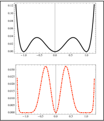
Figure 1: The potentials for the standard and generalized models, plotted in function of the Higgs field, with black/higher and red/lower lines, respectively.

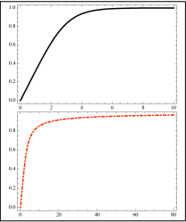
Figure 2: The Higgs field as a function of the distance $r$ for the standard and generalized models. Conventions as in Fig1. Note that in our model the vacuum is reached for a larger distance than in the standard model – see Fig.3 as well

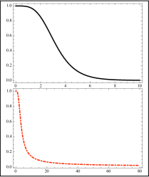
Figure 3: The spatial component of the gauge field. Conventions as in Fig. 2.

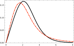
Figure 4: The electric field in units of $e$ (black/ red-dotdashed lines for standard/our model). This is also the Figure for the polar current density $j^{\theta}$ in units of $k$. Note that it is smaller and spread over a larger distance than in the standard model.

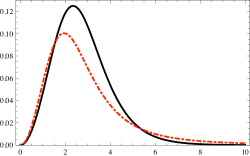
Figure 5: The magnetic field in units of $e$. Note that it is smaller and spread over a larger distance than in the standard model. The same result applies for the charge density $\rho$. Conventions as in Fig. 4.

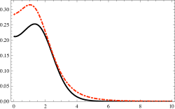
Figure 6: The energy density. Conventions as in Fig. 1.

VI Ending comments

In this work we have studied the presence of vortices in a generalized Chern-Simons model. The idea is different from the recent work Babichev1 , where the author has investigated vortices in the Maxwell-Higgs model, modified to accommodate generalized structure, with the kinetic term being changed to a function of it. This study was done with the numerical integration of the equations of motion, and the modification there introduced has induced another mass scale.

Here, our objective was to generalize the Chern-Simons model in a way such that we could find first order differential equations. To do this, we have changed the kinetic term $|D_{\mu}\varphi|^{2}$ to $w(|\varphi|)|D_{\mu}\varphi|^{2}$. We suppose that this modification leads to an effective planar field theory somehow similar to the standard Chern-Simons model. Despite the modification in the kinematic scalar field term, we could write a first order framework and find vortices which are qualitatively similar to the vortices of the standard Chern-Simons model. However, we could identify several properties of the BPS vortices which are quantitatively different from the standard vortices, since the solutions can be thicker then the standard solutions. These differences are shown in all the figures, where we depict distinct features of the vortices in both the generalized and standard Chern-Simons models.

When compared to the model investigated in Babichev1 , an important distinction which appears in our work is that the modification we have included does not introduce another mass scale in the system. To see this clearly, let us write the potential in Eq. (53) in terms of dimensional quantities. It writes

$$V(|\varphi|)=\frac{3\,e^{4}}{k^{2}v^{6}}|\varphi|^{2}(v^{2}-|\varphi|^{2})^{8}$$ (62)

where $v$ is the symmetry breaking parameter of the model. In this case, the mass scale $M$ which we had to include at the end of Sec. II can be seen as $M=v^{2}$, so we do not need an extra mass scale, which had to be included in Babichev1 .

We are now examining how to obtain first order equations in a more general model, modifying the kinetic scalar field term but including both the Maxwell and the Chern-Simons terms. Also, we are studying the presence of vortices in a Maxwell-Higgs model with the k-field modification similar to the case investigated in Babichev1 . Preliminary results indicate the presence of compact vortices, e.g., of vortices with the scalar and gauge fields getting to their vacuum values at finite distances from the origin.

Before ending the work, let us study the Bogomol’nyi decomposition of the energy of the static solutions of the first order equations found above. To make the calculation explicit, we rewrite the energy density (13) in the form

$$\varepsilon = w\left|\left(D_{1}\pm iD_{2}\right)\varphi\right|^{2}+\left(\frac{kB}{2eg\sqrt{w}}\mp\sqrt{V}\right)^{2}$$ (63)

$$\;\;\;\pm ewg^{2}B\pm\frac{kB}{eg}\sqrt{\frac{V}{w}}\pm\frac{w}{r}\frac{d}{dr}\left(g^{2}a\right)\text{ .}$$

This result can be used to recover the standard case of the Chern-Simons model. We make $w\left(g\right)=1$ to get to

$$\varepsilon = \left|\left(D_{1}\pm iD_{2}\right)\varphi\right|^{2}+\left(\frac{kB}{2eg}\mp\frac{e^{2}}{k}g\left(g^{2}-1\right)\right)^{2}$$ (64)

$$\;\;\;\pm eB\pm\frac{1}{r}\frac{d}{dr}\left(g^{2}a\right)\text{ ,}$$

with the standard potential

$$V=\frac{e^{4}}{k^{2}}g^{2}\left(1-g^{2}\right)^{2}\text{,}$$ (65)

which leads to the first order equations obtained in Sec. III.

On the other hand, if we take $w\left(g\right)=3\,(1-g^{2})^{2}$ we get

$$\varepsilon = 3\left(1-g^{2}\right)^{2}\left|\left(D_{1}\pm iD_{2}\right)\varphi\right|^{2}\mp\frac{1}{r}\frac{d}{dr}\left(a\left(1-g^{2}\right)^{3}\right)$$ (66)

$$+\left(\frac{kB}{2eg\sqrt{3}\left(1-g^{2}\right)}\mp\frac{\sqrt{3}e^{2}}{k}g\left(1-g^{2}\right)^{4}\right)^{2}\text{ ,}$$

where we used

$$V=\frac{3e^{4}}{k^{2}}g^{2}\left(1-g^{2}\right)^{8}\text{ .}$$ (67)

We point out that an integration of $r^{-1}d_{r}\left(a\left(1-g^{2}\right)^{3}\right)$ over all planar space can be identified with an integration of $-B(r)$ the same space. This integration process gives the magnetic flux $\phi$ which is topologically invariant. In this way, this result leads to the first order equations used above, so the corresponding solutions are in fact BPS states, with the energy bound being $E_{B}=e\,|\phi|$ where $\phi$ represents the flux of the magnetic field in the plane. We note that the energy bound in the generalized model is the same of the energy bound of the standard Chern-Simons model.

VII Acknowledgments

We thank CAPES and CNPq, Brazil and Christoph Adam and Filipe Correia for interesting comments. C dos Santos is partially financed by SFRH/BSAB/925/2009, FCT Grant No. CERN/FP/109306/2009. and would like to thank the Departamento de Fisica USC for all their hospitality while doing this work.

References

- (1) J. Hong, Y. Kim, P.Y. Pac, Phys. Rev. Lett. 64, 2230 (1990).
- (2) R. Jackiw, E. J.Weinberg, Phys. Rev. Lett. 64, 2234 (1990).
- (3) R. Jackiw, K. Lee, E. J.Weinberg Phys. Rev. D 42, 3488 (1990).
- (4) G. V. Dunne, Self-Dual Chern-Simons Theories, (Springer, Heidelberg, 1995).
- (5) G. V. Dunne, Aspects of Chern-Simons Theory, Les Houches Lectures, 1998 [hep-th/9902115].
- (6) N. Sakai, D. Tong, JHEP 0503, 019 (2005).
- (7) G. S. Lozano, D. Marques, E. F. Moreno, F. A. Schaposnik, Phys. Lett. B 654, 27 (2007).
- (8) T. H. R. Skyrme, Proc. R. Soc. London, Ser. A 260, 127 (1961).
- (9) L. Faddeev, A.J. Niemi Phys. Rev. Lett. 82, 1624, (1999).
- (10) D. A. Nicole, J. Phys. G 4 1363, (1978 ).
- (11) S. Deser, M. J. Du?, C. J. Isham, Nucl. Phys. B 114 29 (1976).
- (12) H. Aratyn, L. A. Ferreira, A. H. Zimerman, Phys. Rev. Lett. 83 1723, (1999).
- (13) D. Bazeia, J. Menezes, and R. Menezes, Phys. Rev. Lett. 91, 241601 (2003).
- (14) C. Adam, J. Sanchez-Guillen, R. A. Vazquez and J. A. Wereszczynski, Math. Phys. 47, 052302 (2006).
- (15) E. Babichev, V. Mukhanov, A. Vikman, JHEP 2, 101, (2008).
- (16) C. Armendariz-Picon, V. F. Mukhanov, P. J. Steinhardt, Phys. Rev. D 63, 103510, (2001).
- (17) C. Adam, N. Grandi, J. Sanchez-Guillen, A. Wereszczynski, J. Phys. A 41, 212004 (2008). Erratum-ibid. A 42, 159801 (2009).
- (18) C. Adam, J. Sanchez-Guillen, A. Wereszczynski, J.Phys.A40, 13625, (2007); Erratum-ibid. A 42, 089801 (2009).
- (19) C. Adam, N. Grandi, P. Klimas, J. Sanchez-Guillen, A. Wereszczynski, J. Phys. A 41, 375401 (2008).
- (20) C. Adam, P. Klimas, J. Sanchez-Guillen, A. Wereszczynski, J. Phys. A 42, 135401 (2009).
- (21) C. Adam, N. Grandi, P. Klimas, J. Sanchez-Guillen, A. Wereszczynski, [arXiv:0908.0218]
- (22) G. H. Derrick, J. Math. Phys. 5, 1252 (1964).
- (23) E. Babichev, Phys. Rev. D 77 065021 (2008).
- (24) X. Jin, X. Li, D. Liu, Class. Quantum Grav. 24, 2773 (2007).
- (25) S. Sarangi, J. High Energy Phys. 018, 0807 (2008).
- (26) D. Bazeia, R. Menezes, A. Yu. Petrov, Phys. Lett. B 683, 335 (2010), [arXiv:0910.2827].
- (27) D. Bazeia, A. R. Gomes, L. Losano, R. Menezes, Phys. Lett. B 671, 402 (2009).
- (28) D. Bazeia, L. Losano, R. Menezes, Phys. Lett. B 668, 246 (2008).
- (29) D. Bazeia, L. Losano, R. Menezes, J.C.R.E. Oliveira, Eur. Phys. J. C 51, 953 (2007).
- (30) E. Babichev, Phys. Rev. D 74, 085004 (2006).
- (31) E. Babichev, P. Brax, C. Caprini, cesJEP 3, 091 (2009).
- (32) E. Bogomol’nyi, Sov. J. Nucl. Phys. 24, 449 (1976).
- (33) M. Prasad, C. Sommerfield, Phys. Rev. Lett. 35, 760 (1975).
- (34) H. Vega, F. Schaposnik, Phys. Rev. D 14, 1100 (1976).
- (35) P. Rosenau, J.M. Hyman, Phys. Rev. Lett. 70, 564 (1993).
- (36) F. Cooper, H. Shepard, P. Sodano, Phys. Rev. E 48, 4027 (1993).
- (37) A. Khare, F. Cooper, Phys. Rev. E 48, 4843 (1993).
- (38) F. Cooper, J.M. Hyman, A. Khare, Phys. Rev. E 64, 026608 (2001).
- (39) A. Zee, Prog. Theor. Phys. Suppl. 107, 77 (1992).
- (40) A. Vilenkin, E. P. S. Shellard, Cosmic Strings and Other Topological Defetcs, Cambridge University Press, Cambridge, UK (1994).