Dynamically avoiding fine-tuning the cosmological constant: the “Relaxed Universe”

Abstract:

We demonstrate that there exists a large class of ${\cal F}(R,{\cal G})$ action functionals of the scalar curvature and of the Gauß-Bonnet invariant which are able to relax dynamically a large cosmological constant (CC), whatever it be its starting value in the early universe. Hence, it is possible to understand, without fine-tuning, the very small current value $\Lambda_{0}\sim H_{0}^{2}$ of the CC as compared to its theoretically expected large value in quantum field theory and string theory. In our framework, this relaxation appears as a pure gravitational effect, where no ad hoc scalar fields are needed. The action involves a positive power of a characteristic mass parameter, ${\cal M}$, whose value can be, interestingly enough, of the order of a typical particle physics mass of the Standard Model of the strong and electroweak interactions or extensions thereof, including the neutrino mass. The model universe emerging from this scenario (the “Relaxed Universe”) falls within the class of the so-called $\Lambda$XCDM models of the cosmic evolution. Therefore, there is a “cosmon” entity $X$ (represented by an effective object, not a field), which in this case is generated by the effective functional ${\cal F}(R,{\cal G})$ and is responsible for the dynamical adjustment of the cosmological constant. This model universe successfully mimics the essential past epochs of the standard (or “concordance”) cosmological model ($\Lambda$CDM). Furthermore, it provides interesting clues to the coincidence problem and it may even connect naturally with primordial inflation.

1 Introduction

The status of cosmology as a quantitative subdiscipline of physics is largely based on the high-quality observations made during the last two decades. The availability of these data enabled cosmologists to demonstrate that cosmological models are able to explain not only qualitative features of the universe and its dynamics, but also quantitatively reproduce the details of the many observed cosmic phenomena [1]. Yet, the discovery of the accelerated expansion of the universe at the present epoch [2] revealed a gap in our understanding of the universe. The search for the underlying mechanism producing the accelerated expansion revived an old problem of theoretical physics: the cosmological constant problem [3, 4], which manifests itself as the double conundrum on the tiny observed value of the cosmological constant (CC) in Einstein’s equations – the “old CC problem” [5] – and the puzzling fact that this value is so close to the current matter density – the “cosmic coincidence problem” [6]. Even though the simplest candidate for the acceleration mechanism is the existence of a small positive cosmological constant, $\Lambda$, now incorporated into the benchmark model of modern cosmology, or “concordance” $\Lambda$CDM model, there is quite a list of challenging cosmological problems of various sorts afflicting the standard model of cosmology, see e.g. [7].

Above all these problems there is a problem of greatest importance, one which is by far the most troublesome one from the point of view of Fundamental Physics, to wit: the size of the cosmological constant energy density required to describe the cosmological data is in drastic disaccord with the value predicted by any known fundamental physical theory based on quantum field theory (QFT) or string theory. Indeed, from a theoretical point of view, the cosmological constant energy density, $\rho_{\Lambda}=\Lambda/(8\pi G_{N})$ ($G_{N}$ being Newton’s constant), is a single number, but of remarkable composition as it involves all sources of vacuum energy: e.g. the zero-point energy density of a quantum field of mass $m$ produces a contribution to the CC energy density of the order of $m^{4}$, where bosonic fields contribute positively and fermionic fields negatively; phase transitions in the early universe also leave an imprint on the value of $\rho_{\Lambda}$ in the form of vacuum energy associated to spontaneous symmetry breaking (e.g. the energy density of the electroweak vacuum); or the non-perturbative condensates (as e.g. the quark and gluon condensates of the QCD vacuum) etc. All these contributions, which differ in size and sign, have a common characteristic: they are all much larger in absolute value than the experimentally determined vacuum energy density, $\rho_{\Lambda}^{0}\simeq(2.3\times 10^{-3}\,\text{eV})^{4}$ [1]. There is a (remote) possibility that these manyfold effects might cancel among themselves to produce the observed value of the CC. This, however, requires extreme fine-tuning which, in perturbative QFT, needs to be iterated to all orders of the perturbative expansion. Such explanation, therefore, although technically possible, is utterly unconvincing.

If we discard the explanations based on fine-tuning, and we take seriously the idea that all the contributions to the vacuum energy do have an impact on the final CC value, then we are unavoidably left with a value of $\rho_{\Lambda}$ many orders of magnitude larger than $\rho_{\Lambda}^{0}$. Since we have no experimental verification of the dynamics in the UV limit, the size and sign of the “initial” CC energy density – which we may call $\rho_{\Lambda}^{i}$ – are not precisely known, except the fact that its absolute value must be really huge when measured in units of the observed CC energy density; i.e. the number $|\rho_{\Lambda}^{i}|/\rho_{\Lambda}^{0}$ must be enormous.

To reconcile the anomalously large size of this ratio with the behavior of the observed universe, the value of $\rho_{\Lambda}^{i}$ has to be neutralized in some reasonable manner. One possibility would be the existence of a mildly broken symmetry requiring the CC to be very small (zero if the symmetry would be exact). Such a symmetry, however, is not presently known. Supersymmetry (SUSY) [8], for instance, despite the first natural hopes [9], cannot cure the CC problem in any obvious way, because we know that SUSY must be broken at the electroweak scale or higher, which means that the SUSY particles must have masses larger than their conventional counterparts, and as a result the “residual” vacuum energy left in the universe must again be of the order (or even larger) than that of the Standard Model (SM) of particle physics, i.e. of order $M_{W}^{4}$, where $M_{W}\sim 100$ GeV is the scale of the weak gauge boson masses . Therefore, in general we expect, roughly, $|\rho_{\Lambda}^{i}|/\rho_{\Lambda}^{0}\sim 10^{55}$, which is an appallingly large number! Obviously, a theoretical breakthrough is demanded to account for this situation.

From a physical point of view, it is especially appealing to have a dynamical adjustment of the CC value, because we can then avoid resorting to too preposterous a fine-tuning of the parameters – at least 55 digits in the SM case. This idea was originally pursued in terms of dynamical scalar fields [12], but it was later shown by S. Weinberg that it is generally obstructed by a “no-go theorem” [3]. Subsequently, the more modest idea of quintessence [13] was proposed without attempting to explain the smallness of the CC, but only to cope with some aspects of the cosmic coincidence problem.

In this paper, we wish to face a possible dynamical solution that can escape the no-go theorem and that is based on a different concept, one that makes no use of scalar fields. Specifically, we refer to the concept of “dynamical effective $\Lambda$” or “effective vacuum energy” $\rho_{\Lambda{\rm eff}}$, in which, rather than replacing $\Lambda$ by a collection of ad hoc ersatz fields, we stick to the idea that the CC term in Einstein’s equations is still a “true cosmological term”, although we permit that “the observable CC at each epoch” can be an effective quantity evolving with the expansion of the universe: $\rho_{\Lambda{\rm eff}}=\rho_{\Lambda{\rm eff}}(H)$, where $H$ is the expansion rate or Hubble function. This general dynamical $\Lambda$ approach has been recently re-emphasized in [14, 15], and it was explored with different particular implementations in the past from the point of view of QFT in curved-space time [16, 17], including some recent applications to structure formation [18] – see e.g. the review [19] and references therein.

The variable CC approach was also tried long ago on purely phenomenological terms, cf. [20, 21]. Furthermore, the idea of a slowly running CC is in general compatible with the experimental data [22, 23], and has been even exploited as an alternative description of the notion of dynamical dark energy (DE) for a possible viable solution of the aforementioned cosmic coincidence problem [24, 25, 26]. But, most important of all, it may also be advantageously utilized as a powerful mechanism capable of solving (or highly alleviating) the big or “old” CC problem [3], viz.  the absolutely formidable task of trying to explain the value itself of the current vacuum energy $\rho_{\Lambda}^{0}$ – not just its time evolution in the vicinity of it – on the face of its enormous input value $\rho_{\Lambda}^{i}$ left over in the early times.

Can we explain the measured value of $\Lambda$ and at the same time insure that it remains safely small throughout the entire history of the universe? In this paper, we shall present a thorough attempt of this sort, actually one which substantially improves previous recent attempts along these lines [27, 28]. From now on, we shall call this new process of dynamical neutralization of the “true” cosmological constant: the “relaxation mechanism” of the CC.

Relaxation offers indeed an entirely different perspective on the old CC problem. Many CC adjustment mechanisms, partly discussed above, function unilaterally, as e.g. when using scalar fields. In other words, in these cases the dynamics of the relaxation mechanism works “intrinsically” to neutralize the real value of the CC. A new quality could be added to the relaxation mechanism if it becomes bilateral. Namely, apart from the mechanism itself for neutralizing the value of the CC, we could also envisage that the expansion of the universe, fueled by the big CC value $\rho_{\Lambda}^{i}$, enables the very action of the relaxation mechanism. The idea is that the relaxation mechanism neutralizes the value of $\rho_{\Lambda}^{i}$, but at the same time the existence of this value sets the relaxation mechanism to motion. Since the expansion of the universe should be responsible for the triggering of the relaxation dynamics, it is reasonable to assume that such mechanism should be closely related to the expansion itself, or more precisely, to the interaction governing the expansion, i.e. gravity.

Despite the appeal of such a feedback, a number of important questions have to be answered: i) Is it possible that the observed value of the CC (or effective vacuum energy) is small exactly because the “real” value of the CC is large? ii) Is there a way to dynamically counterbalance the effects of a large CC in all epochs of the cosmic evolution? iii) Can the feedback between the relaxation mechanism and expansion be formulated in terms of an action functional? In this paper, we present a modified gravity theory based on an action functional ${\cal F}(R,{\cal G})$ of the Ricci scalar, $R$, and the Gauss-Bonnet invariant, ${\cal G}$, in which all the above questions have an affirmative answer.

A simple model exploring the viability of a mechanism cancelling dynamically the effects of a large CC was presented in [27]. Previously, it had been shown that the inhomogeneous equation of state (EOS) of a cosmic fluid can be interpreted as an effective description of modified gravity theories or even braneworld models [29]. In a cosmological model containing only two components, a large cosmological constant of an arbitrary sign and a component with an inhomogeneous EOS of the form $p=w\rho-\beta H^{-\alpha}$, for $\alpha>0$ the cosmic expansion asymptotically tends to de Sitter phase with a small positive effective CC [27]. Essentially, the effect of a very large $\Lambda$ is counterbalanced by the terms of the form $1/H^{2n}$ when $H$ is sufficiently small. In this cosmological model, at late times the universe expands as if there existed a small positive CC even though the actual CC is very large and it can even be negative. As there is no fine-tuning in this model, such a dynamical outcome can be rightfully identified as a viable approach for solving the cosmological constant problem. One specific feature of the model deserves a special emphasis. Within this relaxation mechanism, the size of the CC is not only a problem, but also a part of the solution. To illustrate this fact let us consider the asymptotic value of the Hubble parameter $H_{\mathrm{asym}}\sim\sqrt{\Lambda_{\text{eff}}}$ for $\alpha=2$. For this value of $\alpha$ we have $H_{\mathrm{asym}}\sim 1/|\rho_{\Lambda}^{i}|$. The bigger $\rho_{\Lambda}^{i}$ is, the smaller is the effective observed $\Lambda_{\text{eff}}$. For some other recent work on relaxation mechanisms, see also [30] and [31]. For recent alternative ideas on the CC problem, see [32, 33].

The mechanism based on the inhomogeneous EOS, despite exhibiting CC relaxation properties, is incomplete since it does not contain matter or reproduce the observed sequence of epochs in the history of the universe. The idea of the CC relaxation mechanism has to be embedded into a realistic cosmological model. Such a realistic implementation was made in [28] in the formalism of variable $\Lambda$ interacting with a dark matter component, i.e. within the context of the so-called $\Lambda$XCDM model [24]. The variable CC contains contributions in the form of functions of curvature invariants such as $R^{2}$, $R^{ab}R_{ab}$ and $R^{abcd}R_{abcd}$. The model successfully produces the sequence of radiation, matter and de Sitter phases in the expansion of the universe. During the de Sitter phase, the action of a large CC is counterbalanced by the term $1/H^{2n}$ when $H$ is sufficiently small, similarly as with having inhomogeneous EOS. However, during the matter and radiation dominated phases, the effect of a large $\Lambda$ is equilibrated by the terms $\sim 1/(q-1/2)$ and $\sim 1/(q-1)$, respectively, where $q$ is the deceleration parameter. Within this model one can easily produce an expansion history of the universe close to that of the $\Lambda$CDM model despite the persistence of the huge primeval CC, which is permanently subdued by the dynamical mechanism. Besides, a dedicated analysis of the growth of perturbations shows that the formation of structures in this kind of models is also comparable to the $\Lambda$CDM [34].

The model introduced and elaborated in [28] is thus phenomenologically very successful, but it lacks the action principle formulation. To fill this remaining gap, we proposed recently a specific model universe [35] based on an action functional for modified gravity. In the present paper, we extend and generalize this approach while maintaining the phenomenologically pleasing features discussed above. Specifically, we discuss here a modified gravity theory (“The Relaxed Universe”) based on a class of ${\cal F}(R,{\cal G})$ action functionals capable of relaxing the highly “stressed” primeval state of our universe, namely a state which is beset by a large vacuum energy which prevents the startup of the normal thermal history. The relaxation mechanism allows not only to unblock this situation, it also operates very actively during all the subsequent epochs of the cosmic expansion without fine-tuning the parameters of the theory at any time. Furthermore, it involves a characteristic mass scale, ${\cal M}$, whose value is of the order of a typical particle physics scale whether of the SM or of a Grand Unified Theory (GUT), and therefore avoids introducing extremely tiny masses ($m_{\phi}\sim H_{0}\sim 10^{-33}$ eV) plaguing most proposals, as e.g. quintessence [13].

It should finally be emphasized that the cosmological model introduced here goes beyond the idea of modified gravity with late time cosmic acceleration [36, 37]. Indeed, let us stress once more that the proposed gravity modifications inherent to our mechanism are crucial during the entire cosmic history, and not just in the late universe. The reason is that they primarily counterbalance the effect of a huge CC during all accessible epochs (radiation and matter), and without any fine-tuning. The late time acceleration phenomenon appears here only as a special, but certainly very important effect, either in quintessence-like, de Sitter or phantom-like disguise.

The paper is organized as follows. In the next section, we sketch the old CC problem and its relation with the notion of fine-tuning. In section 3 we define and solve the ${\cal F}(R,{\cal G})$-cosmology. In section 4 we discuss the working principle of the relaxation mechanism. The analysis of some concrete implementations of the model is performed in section 5, including detailed numerical results. In the last section we deliver our conclusions. Finally, in appendix A we provide information on our notation and conventions, in appendix B we extend the discussion of the severity of the CC fine-tuning problem in QFT, and in appendix C we briefly discuss the relaxation mechanism in the solar system.

2 The old CC problem as a fine-tuning problem

Before we present our relaxation mechanism, let us summarize the old CC problem and discuss why the fine-tuning problem unavoidably appears if one does not modify some aspects of the theory of gravity in interaction with matter. We wish to illustrate the problem within the context of the standard model (SM) of particle physics, and more specifically within the Glashow-Weinberg-Salam model of electroweak interactions. This is the most successful QFT we have at present (together with the QCD theory of strong interactions), both theoretically and phenomenologically, and therefore it is the ideal scenario where to formulate the origin of the problem. As is well-known, the unification of weak and electromagnetic interactions into a renormalizable theory requires to use the principle of local gauge symmetry in combination with the phenomenon of spontaneous symmetry breaking (SSB). It is indeed the only known way to generate all the particle masses by preserving the underlying gauge symmetry. In the SM, one must introduce a fundamental complex doublet of scalar fields. However, in order to simplify the discussion, let us just consider a field theory with a real single scalar field $\varphi$, as this does not alter at all the nature of the problem under discussion. To trigger SSB, one must introduce a potential for the field $\varphi$, which in renormalizable QFT takes the form (the tree-level Higgs potential):

$$V(\varphi)=\frac{1}{2}\,m^{2}\,\varphi^{2}+\frac{1}{4!}\,\lambda\,\varphi^{4}\,,\ \ \ \ \ (\lambda>0)\,.$$ (1)

Since we are dealing with a problem related with the CC, we must inexcusably consider the influence of gravity. To this effect, we shall conduct our investigation of the CC problem within the semiclassical context, i.e. from the point of view of quantum field theory (QFT) in curved space-time [38]. It means that we address the CC problem in a framework where gravity is an external gravitational field and we quantize matter fields only [14, 39]. The potential in equation (1) is given at the moment only at the classical level, but it will eventually acquire quantum effects generated by the matter fields themselves. In this context, we need to study what impact the presence of such potential may have on Einstein’s equations both at the classical and at the quantum level.

Einstein’s field equations for the classical metric in vacuo are derived from the Einstein-Hilbert (EH) action with a cosmological term $\Lambda_{\rm vac}$ (hereafter the CC vacuum term). The EH action in vacuo reads:

$$S_{EH}=\frac{1}{16\pi\,G_{N}}\,\int d^{4}x\sqrt{|g|}\,\left(\,R-2\,\Lambda_{\rm vac}\,\right)=\,\int d^{4}x\sqrt{|g|}\,\left(\frac{1}{16\pi\,G_{N}}\,R-\rho_{\Lambda\rm vac}\right)\,.$$ (2)

(See the Appendix A for our notation and sign conventions). Here we have defined $\rho_{\Lambda\rm vac}$, the energy density associated to the CC vacuum term:

$$\rho_{\Lambda\rm vac}=\frac{\Lambda_{\rm vac}}{8\pi\,G_{N}}\,.$$ (3)

The classical action including the scalar field $\varphi$ with its potential (1) is

$$S=S_{EH}+\int d^{4}x\,\sqrt{|g|}\,\left[\frac{1}{2}\,g^{ab}\,\partial_{a}\varphi\,\partial_{b}\varphi-V(\varphi)\right]\,.$$ (4)

Due to the usual interpretation of Einstein’s equations as an equality between geometry and a matter-energy source, it is convenient to place the $\rho_{\Lambda\rm vac}$ term as a part of the matter action, $S[\varphi]$. Then the total action (4) can be reorganized as

$$S=\,\frac{1}{16\pi\,G_{N}}\,\int d^{4}x\sqrt{|g|}\,R+S[\varphi]\,,$$ (5)

with

$$S[\varphi]=\int d^{4}x\,\sqrt{|g|}\,\left[\frac{1}{2}\,g^{ab}\,\partial_{a}\varphi\,\partial_{b}\varphi-\rho_{\Lambda\rm vac}-{V}(\varphi)\right]\equiv\int d^{4}x\,\sqrt{|g|}\ \mathcal{L}_{\varphi}\,,$$ (6)

where $\mathcal{L}_{\varphi}$ is the matter Lagrangian for $\varphi$. For the moment, we will treat the matter fields contained in $\mathcal{L}_{\varphi}$ as classical fields, and in particular the potential $V$ is supposed to take the classical form (1) with no quantum corrections. If we compute the energy-momentum tensor of the scalar field $\varphi$ in the presence of the vacuum term $\rho_{\Lambda\rm vac}$, let us call it $\tilde{T}_{ab}^{\varphi}$, we obtain

$$\tilde{T}_{ab}^{\varphi}={2\over\sqrt{|g|}}\,{\delta\,S[\varphi]\over\delta\,g^{ab}}=2\,{\partial\mathcal{L}_{\varphi}\over\partial\,g^{ab}}-g_{ab}\,\mathcal{L}_{\varphi}=g_{ab}\,\rho_{\Lambda\rm vac}+{T}_{ab}^{\varphi}\,,$$ (7)

where we have used $\partial\sqrt{|g|}/\partial g^{ab}=-(1/2)\sqrt{|g|}\,g_{ab}$. Here

$${T}_{ab}^{\varphi}=\left[\,\partial_{a}\varphi\,\partial_{b}\varphi-\frac{1}{2}\,g_{ab}\ \partial_{c}\varphi\,\partial^{c}\varphi\right]+g_{ab}\,V(\varphi)$$ (8)

is the ordinary energy-momentum tensor of the scalar field $\varphi$.

In the vacuum (i.e. in the ground state of $\varphi$) there is no kinetic energy, so that the first term on the r.h.s of (8) does not contribute in that state. Only the potential may take a non-vanishing vacuum expectation value, which we may call $\langle V(\varphi)\rangle$. Thus, the ground state value of (7) is

$$\langle\tilde{T}_{ab}^{\varphi}\rangle=g_{ab}\,\rho_{\Lambda\rm vac}+\langle{T}_{ab}^{\varphi}\rangle=g_{ab}\,(\rho_{\Lambda\rm vac}+\langle V(\varphi)\rangle)\equiv\rho_{\rm vac}^{\rm cl}\ g_{ab}\,,$$ (9)

where $\rho_{\rm vac}^{\rm cl}$ is the classical vacuum energy in the presence of the field $\varphi$.

If $m^{2}>0$ in equation (1), then $\langle\varphi\rangle=0\ \Rightarrow$ $\langle V(\varphi)\rangle=0$ and the classical vacuum energy is just the original $\rho_{\Lambda\rm vac}$ term,

$$\langle\tilde{T}_{ab}^{\varphi}\rangle=g_{ab}\,\rho_{\Lambda\rm vac}\,.$$ (10)

This result also applies in the free field theory case. However, if the phenomenon of SSB is active, which precisely occurs when $m^{2}<0$, we have a non-trivial ground-state value for $\varphi$:

$$\langle\varphi\rangle=\sqrt{\frac{-6\,m^{2}}{\lambda}}\,.$$ (11)

In this case, there is an induced part of the vacuum energy at the classical level owing to the electroweak phase transition generated by the Higgs potential. This transition induces a non-vanishing contribution to the cosmological term which is usually called the “induced CC”. At the classical level, it is given by

$$\rho_{\Lambda\rm ind}\equiv\langle V(\varphi)\rangle=-\frac{3\,m^{4}}{2\lambda}=-\frac{1}{8}\,M_{\cal H}^{2}\,\langle\varphi\rangle^{2}=-\frac{1}{8\sqrt{2}}\,M_{\cal H}^{2}\,M_{F}^{2}\,,$$ (12)

In the last two equalities, we have used the physical Higgs mass squared $M_{\cal H}^{2}=-2m^{2}>0$. Indeed, if we redefine the Higgs field as $\cal H=\varphi\,-\langle\varphi\rangle$, then its value at the minimum will obviously be zero. This is the standard position for the ground state of the field before doing perturbation theory. The physical mass is just determined by the oscillations of $\cal H$ around this minimum, i.e. it follows from the second derivative of $V$ at $\varphi=\langle\varphi\rangle$. We have also introduced the so-called Fermi’s scale $M_{F}\equiv G_{F}^{-1/2}\simeq 290\,\text{GeV}$, which is defined from Fermi’s constant obtained from muon decay, $G_{F}\simeq\text{1.166}\times 10^{-5}\,\text{GeV}^{-2}$.

In view of the previous SSB contribution, it is clear that we must replace ${T}_{ab}^{\varphi}\to\tilde{T}_{ab}^{\varphi}$ in the expression of Einstein’s equations in vacuo. Furthermore, in the presence of incoherent matter contributions (e.g. from dust and radiation) described by a perfect fluid we have the additional term $T_{ab}=(\rho+p)u_{a}u_{b}-p\,g_{ab}$. Therefore, Einstein’s equations in terms of coherent and incoherent contributions of matter, plus the vacuum energy of the fields, finally read

$$R_{ab}-\frac{1}{2}g_{ab}R=-8\pi\,G_{N}\,\left(\langle\tilde{T}_{ab}^{\varphi}\rangle+T_{ab}\right)=-8\pi\,G_{N}\,\left[g_{ab}\left(\rho_{\Lambda\rm vac}+\rho_{\Lambda\rm ind}\right)+T_{ab}\right]\,.$$ (13)

We conclude that the “physical value” of the CC, at this stage, is not just the original term $\rho_{\Lambda\rm vac}$, but

$$\rho_{\Lambda{\rm ph}}=\rho_{\Lambda\rm vac}+\rho_{\Lambda\rm ind}\,,$$ (14)

where the induced part is given by (12). However, it is pretty obvious that a severe fine tuning problem is conjured in equation (14) when we compare theory and experiment. Indeed, the lowest order contribution from the Higgs potential, as given by equation (12), is already much larger than the observational value of the CC. Using the LEP lower bound on the Higgs mass ($M_{\cal H}\gtrsim 114\,\text{GeV}$), equation (12) yields $\rho_{\Lambda\rm ind}\simeq-10^{8}\,\text{GeV}^{4}$. Roughly speaking, the VEV of the Higgs potential is (naturally) in the ballpark of the fourth power of the electroweak VEV, i.e. $\rho_{\Lambda\rm ind}\sim v^{4}$, where $v={\cal O}(100)$ GeV. Thus, being the CC observed value of order $\rho_{\Lambda}^{0}\sim 10^{-47}$ GeV⁴, the electroweak vacuum energy density is predicted to be $55$ orders of magnitude larger than $\rho_{\Lambda}^{0}$!

Suppose that the induced result would exactly be $\rho_{\Lambda\rm ind}=-10^{8}\,\text{GeV}^{4}$ and that the vacuum density would exactly be $\rho_{\Lambda}^{0}=+10^{-47}\,\text{GeV}^{4}$. In such case one would have to choose the vacuum term $\rho_{\Lambda\rm vac}$ in equation (14) with a precision of $55$ decimal places in order to fulfill the equation

$$10^{-47}\,\text{GeV}^{4}=\rho_{\Lambda\rm vac}+\rho_{\Lambda\rm ind}=\rho_{\Lambda\rm vac}-10^{8}\,\text{GeV}^{4}\,.$$ (15)

This is of course the famous fine-tuning problem. This problem is in no way privative of the cosmological constant approach to the DE, but it is virtually present in any known model of the DE, in particular also in the quintessence approach [13]. Indeed, the quintessence scalar field potential $V(\varphi)$ is supposed to precisely match the value of the measured DE density at present starting from a high energy scale, usually some GUT scale $\varphi=M_{X}\sim 10^{16}$ GeV. In order to achieve this, an ugly fine-tuning of its initial value $\langle V\rangle\sim 10^{64}$ GeV⁴ is unavoidable. Therefore, the quintessence approaches, apart from introducing extremely unnatural small mass scales of the order of the Hubble function at present (hence masses as small as $m_{\varphi}\sim 10^{-33}$ eV), are plagued with fine-tuning problems in no lesser degree than the original CC problem itself.

However, this is not quite the end of the story yet. In QFT the induced value of the vacuum energy is much more complicated than just the simple result (12), and the fine-tuning problem is much more cumbersome than the one expressed in equation (15), see the Appendix B for a more detailed exposition. At the end of the day, we really need some mechanism that is able to concoct the tuning “dynamically”, i.e. automatically, and without requiring the intervention of some carefully “designed” counterterm encoding the aforementioned fabulous numerical precision. In the rest of the paper, we will try to convince the reader that such mechanism to avoid fine-tuning does exist.

3 ${\cal F}(R,{\cal G})$-cosmology

As already mentioned, in Ref. [28] we investigated a powerful mechanism for relaxing dynamically the vacuum energy or effective cosmological constant. For all of its virtues, it is nevertheless based on introducing a direct modification of the gravitational part at the level of the field equations, and hence without any obvious connection with an action principle. A deeper step in the theoretical construction process would be to implement it from an action functional. For this reason, we investigate here the CC relaxation mechanism within the context of the ${\cal F}(R,{\cal G})$ modified gravity setup and in the metric formalism, where ${\cal F}$ defines a functional of the Ricci scalar $R$ and the Gauß-Bonnet invariant ${\cal G}$,

$${\cal G}\equiv R^{2}-4R_{ab}R^{ab}+R_{abcd}R^{abcd}\,.$$ (16)

(For more details on notation, see once more the Appendix A). The reason why the higher curvature term is ${\cal G}$ rather than the individual higher derivative components that define it will become clear later.

3.1 The generic class of the $\Lambda$XCDM models

Our theoretical ${\cal F}(R,{\cal G})$ construct is placed within the general class of the so-called $\Lambda$XCDM models of the cosmological evolution [24, 28], in which the cosmological term is supplemented (not replaced!) with an effective entity $X$ at the level of the field equations. The resulting cosmological system is thus characterized by a compound dark energy made out of a (constant or variable) cosmological term $\rho_{\Lambda}$ and the contribution $\rho_{X}$ corresponding to a new entity $X$ (called the “cosmon”). The total DE density (or “effective CC density”) reads

$$\rho_{\Lambda{\rm eff}}=\rho_{\Lambda}+\rho_{X}\,.$$ (17)

In the simplest formulation of the $\Lambda$XCDM model, in which Newton’s coupling $G_{N}$ is constant, this overall DE density is locally and covariantly conserved [24]:

$$\dot{\rho}_{\Lambda{\rm eff}}+3\,H\,(\rho_{\Lambda{\rm eff}}+p_{\Lambda{\rm eff}})=0\,,$$ (18)

where $H(t)\equiv{\dot{a}}/{a}$ is the expansion rate (overdots represent time-derivatives with respect to the cosmic time). We can reexpress this equation in terms of $\omega_{\rm eff}$, the effective EOS of the compound DE system:

$$\dot{\rho}_{\Lambda{\rm eff}}+3\,H\,(1+\omega_{\rm eff})\,\rho_{\Lambda{\rm eff}}=0\,,\ \ \ \omega_{\rm eff}=\frac{p_{\Lambda{\rm eff}}}{\rho_{\Lambda{\rm eff}}}=\frac{p_{\Lambda}+p_{X}}{\rho_{\Lambda}+\rho_{X}}\,,$$ (19)

where $p_{\Lambda}=-\rho_{\Lambda}$ is the CC pressure and $p_{X}$ is the pressure of the cosmon component. It follows that matter is also covariantly conserved.

As emphasized in [24], the cosmon is not to be viewed in general as a field, but as a complex object emerging from the full structure of the effective action. Its dynamics is determined either by suggesting an explicit modification of the effective action, or by providing a particular evolution law for the CC term, $\rho_{\Lambda}=\rho_{\Lambda}(t)$. In either case $\rho_{X}=\rho_{X}(t)$ is then completely determined by the local conservation law (18). This can be further appreciated by rewriting that law as follows:

$$\dot{\rho}_{\Lambda}+\dot{\rho}_{X}+\,3\,H\,(1+\omega_{X})\,\rho_{X}=0\,,$$ (20)

where we have defined the effective EOS of the cosmon: $\omega_{X}=p_{X}/\rho_{X}$. The effective EOS of the compound DE system can now be written as

$$\omega_{\rm eff}=\frac{-\rho_{\Lambda}+\omega_{X}\,\rho_{X}}{\rho_{\Lambda}+\rho_{X}}=-1+(1+\omega_{X})\,\frac{\rho_{X}}{\rho_{\Lambda{\rm eff}}}\,.$$ (21)

In general, both $\omega_{X}$ and $\omega_{\rm eff}$ will be non-trivial functions of the cosmic time or the cosmological scale factor, $a=a(t)$, or the redshift: $z=(1-a)/a$. In the original $\Lambda$XCDM model of Ref. [24], one starts from a given evolution law $\rho_{\Lambda}=\rho_{\Lambda}(H)$ for the CC term, specifically one which is motivated by the presence of quantum corrections, and the EOS parameter $\omega_{X}$ for the cosmon is taken constant. This setup enabled a full analytical treatment and an explicit determination of the cosmon energy density as a function of the redshift, $\rho_{X}=\rho_{X}(z)$. In the present case, however, $\rho_{\Lambda}$ is just a constant (given by the initial $\rho_{\Lambda}^{i}$), and the dynamics of the cosmon – represented by the conservation law (20) – will be completely controlled by the influence of a new gravitational term that modifies the EH action. In fact, the complete action functional is composed, apart from the conventional matter part and the EH term, also of the aforementioned function of the invariants $R$ and ${\cal G}$ – whose contribution to the total action will, for brevity sake, be referred to as the “${\cal F}(R,{\cal G})$-functional”. This functional determines the dynamics of $X$. Notice that the apparent simplification produced by the fact that $\rho_{\Lambda}$ is now just a constant is compensated by the fact that the cosmon EOS will be a complicated function of time or redshift: $\omega_{X}=\omega_{X}(z)$. As a result, a complete analytical treatment will not be possible. The reward, however, will be a powerful formulation of the $\Lambda$XCDM model in which the cosmon will be able to efficiently deal (as its name intends to suggest) with the old CC problem, and specifically with the toughest aspect of it: the fine-tuning problem.

Let us note that the definition of the cosmon $X$ in the wide class of $\Lambda$XCDM models is really very general because it introduces the energy density $\rho_{X}$ not at the core level of the action, but at the level of the field equations. In the present case, our $\Lambda$XCDM model is constructed ab initio at the level of an action functional containing the piece ${\cal F}(R,{\cal G})$. This is of course a great advantage from the theoretical point of view. However, in order to recognize what is $\rho_{X}$ in the present case, and finally unveil the corresponding $\rho_{\Lambda{\rm eff}}$ (i.e. the “effective CC”) that results from the presence of the ${\cal F}$-functional, one has to account for the field equations of the complete effective action. We do this in the next section.

3.2 Action principle and field equations

The complete effective action of our cosmological model reads

$$\mathcal{S}=\int d^{4}x\,\sqrt{|g|}\left[\frac{1}{16\pi G_{N}}R-\rho_{\Lambda}^{i}-{\cal F}(R,{\cal G})+\mathcal{L}_{\phi}\right]\,,$$ (22)

where ${\cal L}_{\phi}$ stands for the Lagrangian of the matter fields. Clearly, our functional constitutes an extension of the EH action with CC in which we have added the ${\cal F}(R,{\cal G})$ part, i.e. a generalization of equations (5)-(6). We take ${\cal F}$ within the class of functions of the form

$${\cal F}(R,{\cal G})=\beta\,F(R,{\cal G})+A(R)\,,$$ (23)

in which $\beta$ is a parameter, $F(R,{\cal G})$ a non-polynomial function (see below) and $A(R)=a_{2}R^{2}+a_{3}R^{3}...$ is a (low order) polynomial of $R$. The latter has neither linear nor independent term, the reason being that these terms can already be included as part of the EH action with CC. Notice that we do not use ${\cal G}$ in the structure of the polynomial $A$ because the first term would just be ${\cal G}$, which is a topological invariant in four dimensions. As for $F(R,{\cal G})$, we take it as a function of negative mass dimension. We will usually call it the “$F$-term”. The canonical implementation of it is a rational function of $R$ and ${\cal G}$ vanishing as $R$ and ${\cal G}$ are sufficiently large, say

$$F(R,{\cal G})=\frac{1}{B(R,{\cal G})}\,,$$ (24)

with $B(R,{\cal G})$ a polynomial in $R$ and ${\cal G}$. Within this canonical ansatz (which we will adopt for most of our considerations), the complete functional (23) reads

$${\cal F}(R,{\cal G})=\frac{\beta}{B(R,{\cal G})}+A(R)\,.$$ (25)

Since, in the FLRW metric, $F(R,{\cal G})$ defines a functional $\Phi(H)$ of the Hubble function or expansion rate $H(t)\equiv{\dot{a}}/{a}$ and its time-derivatives, we can express the required condition as

$$F(R,{\cal G})=\Phi(H)\to 0\,\ \ \ \text{for}\ \ \ H\gtrsim H_{\rm rad}^{*}\,,$$ (26)

where $H_{\rm rad}^{*}$ is the Hubble rate at the time when the very early radiation period sets in, hence after both inflation and reheating have already taken place. We shall explain the motivation for this condition later on. Since $F(R,{\cal G})$ dies off with curvature, the parameter $\beta$ in equation (23) must have a positive dimension of energy, namely

$$\beta\equiv{\cal M}^{N}\,,\ \ \ \ \text{with}\ \ N>0\,,$$ (27)

where $N=n_{B}+4$ is an integer in which $n_{B}$ is equal to the mass dimension of the $B(R,{\cal G})$ polynomial, and ${\cal M}$ represents some characteristic cosmic mass scale associated to our ${\cal F}$-functional. For instance, if $B(R,{\cal G})$ is a polynomial involving just quadratic terms in $R$ and linear in ${\cal G}$, we would have $N=8$. Notice that if the polynomial $A(R)$ reduces to the monomial $a_{2}R^{2}$, then $a_{2}$ is a dimensionless coefficient. In this case, the only dimensionful scales carried by ${\cal F}$ are $\beta$ and those that might involve $B(R,{\cal G})$ in the form of monomials of $R$ (respect. ${\cal G}$) of order $3$ (respect. 2) or above. The mass scale ${\cal M}$ should have some physical significance, and therefore it will be interesting to check which are the typical values allowed for ${\cal M}$ (depending on the choice of $F$) in order to implement realistically the relaxation mechanism in our Universe. Generalizations of $F=1/B$ offer more possibilities for the mass scale ${\cal M}$ and will be discussed later on in Sec. 5.5.

Another essential ingredient of the effective action (22) is of course the “initial” cosmological constant term

$$\Lambda^{i}=8\pi G_{N}\,\rho_{\Lambda}^{i}\,,$$ (28)

in which $\rho_{\Lambda}^{i}$ stands for all possible vacuum energy density contributions (of arbitrary size) pertinent to “initial” phase transitions in the early universe, e.g. the GUT phase transitions, the electroweak transition, the QCD quark-gluon transition, and in general all vacuum energy density contributions associated to the matter fields (bosonic or fermionic) of the Lagrangian $\mathcal{L}_{\phi}$. For instance, $\rho_{\Lambda}^{i}$ embodies the important electroweak contribution from the SM Higgs potential, i.e. $|\rho_{\rm EW}|\sim M_{F}^{2}\,M_{\cal H}^{2}\sim 10^{8}\,\text{GeV}^{4}$. In addition, $\rho_{\Lambda}^{i}$ integrates the QCD contribution, which is of order $\rho_{\rm QCD}\sim\Lambda_{QCD}^{4}$, with $\Lambda_{QCD}\sim 0.1\,\text{GeV}$. Taken alone, any of these SM contributions from particle physics is enormous as compared to the current value of the CC density, $\rho_{\Lambda}^{0}\sim 10^{-47}\,\text{GeV}^{4}$. On the other hand, $\rho_{\Lambda}^{i}$ may contain much larger contributions; in general it will be dominated by the maximum effect prevailing in the early universe, which should be determined by the strongest GUT phase transition, say $\rho_{\Lambda}^{i}\sim M_{X}^{4}$, with $M_{X}\sim 10^{16}\,\text{GeV}$. At the same time, $\rho_{\Lambda}^{i}$ includes the vacuum term $\rho_{\Lambda\rm vac}$, too, if only for renormalizability reasons. This term is completely free and, in the traditional approach explained in section 2 and Appendix B, it can be used (after renormalization) to fine-tune all the other contributions.

For all of its non-trivial composition, $\rho_{\Lambda}^{i}$ is not yet the physical CC of the ${\cal F}(R,{\cal G})$-cosmology, even though it contains all the ingredients of the traditional approach, i.e. all the terms on the r.h.s. of equation (14). If it were, the tuning that we ought to apply to $\rho_{\Lambda\rm vac}$ to compensate for the energy released during the GUT phase transition would make the $55$-digits-electroweak-tuning described in section 2 pale in comparison, and hence would further increase the severity of the CC problem to the utmost level! But this is not what we shall assume here, so $\rho_{\Lambda\rm vac}$ will be taken as any other contribution, it is not important which one. What is important is that we will not take a special (fine-tuned) value for it (in contrast to the traditional approach, see Appendix B, and we will need not do it at any stage.

How to cut off from the root the unending escalade of fine-tunings plaguing the traditional approach and still render a sound value for the physical CC? A first key appears when we compute the “effective Einstein’s equations” of the ${\cal F}(R,{\cal G})$-cosmology. They emerge from functionally differentiating (22) with respect to the metric, with the result (cf. Appendix A for details):

$$0=2\frac{\delta\mathcal{S}}{\delta g^{ab}}=\int d^{4}x\,\sqrt{|g|}\left[\frac{1}{8\pi G_{N}}G_{ab}+g_{ab}\,\rho_{\Lambda}^{i}+2E_{ab}+T_{ab}\right],$$ (29)

where the surface terms have been omitted. Therefore, instead of (13) we now have

$$G_{\,\,b}^{a}=-8\pi G_{N}\left[\rho_{\Lambda}^{i}\,\delta_{\,\,b}^{a}+2E_{\,\,b}^{a}+T_{\,\,b}^{a}\right]\,.$$ (30)

Apart from the Einstein tensor $G_{\,\,b}^{a}=R_{\,\,b}^{a}-({1}/{2})\,\delta_{\,\,b}^{a}\,R$, we have the constant vacuum energy $\rho_{\Lambda}^{i}$ and the energy-momentum tensor $T_{ab}$ of matter. Notice that we have already absorbed in $\rho_{\Lambda}^{i}$ the vacuum effects (e.g. phase transitions and quantum effects) associated to the coherent matter contributions from the fields $\phi$ in the Lagrangian. Therefore,  $T_{ab}$ in equation (29) involves only the incoherent matter contributions. Finally, there is a new (“extra”) gravitational tensor $E_{\,\,b}^{a}$ coming solely from the ${\cal F}(R,{\cal G})$-term in the action (22), which we have also placed on the r.h.s. of the field equations in order not to distort the standard Einstein part, usually positioned on the l.h.s.

On a spatially flat FLRW background with line element $ds^{2}=dt^{2}-a^{2}(t)d\vec{x}^{2}$, scale factor $a(t)$ and expansion rate $H(t)\equiv{\dot{a}}/{a}$, the tensor components of the various gravitational parts in (30) are given by

$$G_{\,\,0}^{0} = -3H^{2}$$

$$G_{\,\,j}^{i} = -\delta_{\,\,j}^{i}(2\dot{H}+3H^{2})\,,$$ (31)

and

$$E_{\,\,0}^{0} = \frac{1}{2}\left[{\cal F}(R,{\cal G})-6(\dot{H}+H^{2}){\cal F}^{R}+6H\dot{{\cal F}}^{R}-24H^{2}(\dot{H}+H^{2}){\cal F}^{{\cal G}}+24H^{3}\dot{{\cal F}}^{{\cal G}}\right]$$ (32)

$$E_{\,\,j}^{i} = \frac{1}{2}\,\delta_{\,\,j}^{i}\left[{\cal F}(R,{\cal G})-2(\dot{H}+3H^{2}){\cal F}^{R}+4H\dot{{\cal F}}^{R}+2\ddot{{\cal F}}^{R}\right.$$ (33)

$$\left.-24H^{2}(\dot{H}+H^{2}){\cal F}^{{\cal G}}+16H(\dot{H}+H^{2})\dot{{\cal F}}^{{\cal G}}+8H^{2}\ddot{{\cal F}}^{{\cal G}}\right],$$

where ${\cal F}^{Y}\equiv\partial F/\partial Y$ are the partial derivatives of ${\cal F}$ with respect to $Y=R,{\cal G}$. Let us remark that in all these expressions the time derivative of the expansion rate can be reexpressed as $\dot{H}=-H^{2}(q+1)$, where

$$q=-\frac{\ddot{a}\,a}{\dot{a}^{2}}$$ (34)

is the deceleration parameter. This quantity will be very important in our discussions, as we shall see immediately. For one thing the two fundamental curvature invariants on which our action functional ${\cal F}$ depends can just be expressed in the FLRW metric in terms of $H$ and $q$ as follows:

$$R=6H^{2}(1-q)\,,\ \ \ \ \ \ \ \ \ \ {\cal G}=-24H^{4}q\,.$$ (35)

Notice from equations (30) and (32) that the effective CC density in our ${\cal F}(R,{\cal G})$-cosmology, and therefore the quantity playing the role of DE in our framework, is not just the parameter $\rho_{\Lambda}^{i}$, but the full expression

$$\rho_{\Lambda{\rm eff}}(H)=\rho_{\Lambda}^{i}+\rho_{\rm ind}(H)\,,$$ (36)

in which

$$\rho_{\rm ind}=2E_{\,\,0}^{0}$$ (37)

constitutes that part of the effective CC which is genuinely induced by the ${\cal F}$-functional. The expression (37) can be called the (gravitationally) “induced dark energy” . It adds up to the original cosmological constant $\rho_{\Lambda}^{i}$ to produce the quantity $\rho_{\Lambda{\rm eff}}$ or “effective vacuum energy density”. The induced DE is obviously dynamical, and with it the total effective DE density too. Therefore, $\rho_{\Lambda{\rm eff}}$ defined by (36) runs with the expansion of the universe. Because of (35), $\rho_{\Lambda{\rm eff}}$ is a function of the expansion rate $H$, the deceleration parameter $q$ and its first time derivative: $\rho_{\Lambda{\rm eff}}=\rho_{\Lambda{\rm eff}}(H,q,\dot{q})$, but for simplicity we shall indicate it sometimes simply as $\rho_{\Lambda{\rm eff}}=\rho_{\Lambda{\rm eff}}(H)$ – as we shall do also with other cosmological quantities. Most important, in the context of the ${\cal F}(R,{\cal G})$-cosmology, the sum (36) is the very observable quantity that should be accessible to observation, as it is this quantity that clearly takes the role of the CC in the effective Einstein’s equations emerging from the action functional (22). Put another way, $\rho_{\Lambda{\rm eff}}$ is the truly “observable DE density” of the ${\cal F}(R,{\cal G})$-cosmology. Notice that we cannot disentangle observationally the two terms in the sum (36), and therefore it does not matter if $\rho_{\Lambda}^{i}$ is very large provided the induced term $\rho_{\rm ind}$ is also large, but with opposite sign, such that the sum (36) leaves a small remainder. Obviously, for this cosmology to be realistic, we expect that this remainder is small enough and moreover runs only mildly with $H$, such that it can mimic approximately the $\Lambda$CDM concordance model. But, at the same time, and in order to avoid the fine-tuning problem, there must be a non-trivial dynamical interplay between the two terms in (36), leaving just a mild running residue at all times of the cosmological evolution after inflation, not just now. Let us remark that models with mildly running cosmological term provide a global fit to LSS and CMB data perfectly comparable to the $\Lambda$CDM model [22].

3.3 Searching for the class of ${\cal F}$ functionals

We will argue that for a realistic approach of the new ${\cal F}(R,{\cal G})$-cosmology, we expect the following two conditions to occur:

1. The effective cosmological term $\rho_{\Lambda{\rm eff}}=\rho_{\Lambda{\rm eff}}(H)$ in equation (36) must essentially coincide with the enormous value of the vacuum energy density in the vicinity of the post-inflationary time, when the seeds of a huge permanent vacuum energy are first sowed – and need to be removed. This value is what defines our big “initial” cosmological constant $\rho_{\Lambda}^{i}$, and corresponds to an epoch characterized by an expansion rate $H\lesssim M_{X}$. The function (23) must, therefore, allow for the following behavior of the quantity (36):

   $$\rho_{\Lambda{\rm eff}}(H)\simeq\rho_{\Lambda}^{i}\lesssim M_{X}^{4}\ \ \ \ \ (H_{\rm rad}^{*}<H\lesssim M_{X})\,.$$ (38)

   That this relation can be amply fulfilled in our framework, can be argued as follows. To start with, remember that we have imposed the condition (26) on the $F$-term. For $H\sim M_{X}$ such condition should presumably be satisfied (because $H_{\rm rad}^{*}\ll M_{X}$), and hence in this range we have

   $${\cal F}(R,{\cal G})\to A(R)=a_{2}R^{2}+...\ \ \ \ \$$ (39)

   where we have taken the simplest non-trivial possibility for the polynomial $A(R)$ in (23). Despite that this term grows with $R$, its value near the startup of the radiation epoch is not sufficiently large yet as to distort the goodness of the condition (38). For instance, for a typical GUT phase transition with $M_{X}\sim 10^{16}\,\text{GeV}$ we have $R\sim H^{2}\sim 8\pi\,\rho_{X}/M_{P}^{2}\sim 8\pi\,M_{X}^{4}/M_{P}^{2}$, and thus

   $$\frac{R^{2}}{\rho_{\Lambda}^{i}}\sim 64\pi^{2}\,\frac{M_{X}^{4}}{M_{P}^{4}}\sim 10^{-9}\,,$$ (40)

   where $M_{P}\equiv G_{N}^{-1/2}\sim 10^{19}\,\text{GeV}$ is the Planck mass. Clearly, the condition (40) would not be so easily satisfied if the vacuum energy left after primordial inflation would be very close to $M_{P}^{4}$. However, it does not seem realistic (not even necessary) to try to extrapolate cosmology up to this point, so we avoid this speculative situation which would probably require a deeper knowledge of the space-time structure at the level of Quantum Gravity rather than QFT in curved space-time (as we are dealing with in our approach). In short, the relaxation mechanism should efficiently wash out the large contributions to the vacuum energy only after inflation has fully accomplished its role, and more specifically after the reheating processes have been able to “restore” the “initial” relativistic matter content of the universe in the form of the so-called “radiation epoch”; but of course not before, since otherwise inflation itself could not have occurred. It follows that for the practical study of the relaxation mechanism we can simplify the induced DE (37) to the reduced form

   $$\rho_{\rm ind}\to\rho_{F}\equiv\rho_{\rm ind}\Big{|}_{A(R)=0}\ \ \ \ (\text{for}\ H<M_{X})\,,$$ (41)

   where the notation $\rho_{F}$ reminds us that this part is totally attributed to the $F$-term with no contributions from the polynomial $A(R)$ in equation (23).

2. At the same time, the effective quantity $\rho_{\Lambda{\rm eff}}(H)$ must not disturb the standard thermal history of the universe, and should reach the present epoch with a value $\rho_{\Lambda{\rm eff}}(H=H_{0})$ very close to $\rho_{\Lambda}^{0}\sim 10^{-47}\,\text{GeV}^{4}$. In view of the fact that $\rho_{\Lambda}^{0}\ll|\rho_{\Lambda}^{i}|$, it means that we need a huge dynamical cancelation between the two terms on the r.h.s. of equation (36) during both the radiation and matter epochs: $\rho_{\rm ind}\simeq-\rho_{\Lambda}^{i}$. On the face of (41), in practice this means that we must have

   $$\rho_{F}\simeq-\rho_{\Lambda}^{i}\,\ \ \ \ \ (\forall\ H\lesssim H_{\rm rad}^{*}\ll M_{X}\ \ \text{until the present})\,.$$ (42)

   This is of course the most delicate point of our construction and relies significantly on a suitable choice of the $F$-term. For example, the choice in equation (24) is convenient because it makes allowance for the requirement

   $$B(R,{\cal G})\to 0\ \ \ \ \ (\forall\ H\lesssim H_{\rm rad}^{*}\ll M_{X}\ \ \text{until the present})\,,$$ (43)

   as a starting point to fulfill the relation (42). Indeed, let us note that the condition (43) insures that $F(R,{\cal G})$ and its derivatives $F^{Y}\,(Y=R,{\cal G})$ become arbitrarily large; in fact as large as $\rho_{\Lambda}^{i}$ might be, but not infinite because $\rho_{\Lambda}^{i}$ is anyway finite and hence the point $B=0$ is actually never reached. How to make the requirement (43) natural (without fine-tuning) such that the relation (42) is fulfilled for arbitrarily large $\rho_{\Lambda}^{i}$, is something that we will discuss in much of the remainder of this paper.

Some further comments are now in order. The aforementioned conditions are interesting in that they not only define the range of the history of the early universe in which the relaxation mechanism of the vacuum energy must operate, they also make clear that the inflationary scenario can be preserved. This setup might actually prepare the ground for triggering primordial inflation itself through an $R^{2}$-term (or a higher order polynomial) in the functional $A(R)$ in equation (25). Indeed, equation (39) is fulfilled for $H>M_{X}$, so that $R^{2}$ becomes dominant in the far UV regime. This is consistent with the fact that the renormalizable quantum theory of matter fields on a curved background must necessarily include the action of vacuum, which contains the higher order $R^{2}$-curvature terms [38]. While these terms are irrelevant for scales of order $M_{X}$ or below – cf. equation (40) – they nevertheless become dominant near the Planck scale, where $R\sim M_{P}^{2}$, and in fact they then furnish the driving force for $R^{2}$-inflation. In other words, the ${\cal F}(R,{\cal G})$-cosmology provides also a possible natural connection with Starobinsky’s inflation [40] and the more recent developments on anomaly-induced inflation [41, 42, 43].

Finally, a possible additional bonus of the polynomial term in (23) is that it may provide an escape to some instability issues discovered in extended gravity theories in the metric formalism [36], as it is known e.g. for ${\cal F}(R)$ and ${\cal F}(R,R_{ab}^{2},R_{abcd}^{2})$ theories [44]. There are also potential difficulties as far as concerns the astrophysical implications on the solar system measurements [36]. In our case, also the functional defined by ${\cal F}(R,{\cal G})$ may not be completely free from typical modified gravity problems [45]. Nevertheless, it behaves better than the general ${\cal F}(R,R_{ab}^{2},R_{abcd}^{2})$-functionals and this should suffice for the illustration purposes of our paper. For example, a remarkable feature of the ${\cal F}(R,{\cal G})$ functionals is that they avoid the Ostrogradski instability, i.e. they do not involve vacuum states of negative energy, and are thought to have a reasonable behavior in the solar system limit [46, 47]. At the same time, Gauß-Bonnet models are automatically free from graviton ghosts and other singularities [47, 48].

From the foregoing considerations, it became clear that the polynomial contribution $A(R)$ is relevant for restoring renormalizability at high energies, for bridging the relaxation framework with inflation and maybe also to help curing stability issues, but the polynomial term is not indispensable for the relaxation mechanism itself. Therefore, we shall hereafter substitute the full ${\cal F}(R,{\cal G})$ functional (23) for its reduced part $\beta\,F(R,{\cal G})$, where the $F$-term is given by (24).

3.4 Effective equation of state

The matter sector can be adequately described by a perfect fluid stress tensor $T_{ab}=(\rho+p)u_{a}u_{b}-p\,g_{ab}$ with four-velocity $u_{a}$, energy density $\rho$ and (isotropic) pressure $p$, respectively. For a fluid at rest ($u^{a}=\delta_{0}^{a}$) this means

$$T_{\,\,0}^{0}=\rho,\,\,\,T_{\,\,j}^{i}=-p\,\delta_{\,\,j}^{i}\,.$$ (44)

Using a fluid description also for the vacuum energy, we define the (effective) pressures corresponding to the induced part (37) through $p_{F}=-(T_{F})_{i}^{i}/3$, where from (30) we have $(T_{F})_{j}^{i}=2\,E_{j}^{i}$. Thus

$$p_{F}=-\frac{2}{3}\,E_{\,\,i}^{i}\,,\ \ \ \ \ p_{\Lambda{\rm eff}}=p_{F}-\rho_{\Lambda}^{i}\,,$$ (45)

where the last expression is the corresponding pressure for the full effective vacuum energy (36). Since the Einstein tensor $G_{ab}$ and the extra gravitational tensor $E_{ab}$ are both covariantly conserved, it follows that the ${\cal F}(R,{\cal G})$-cosmology automatically conserves matter, too, i.e. $\nabla^{a}T_{ab}=0$. Therefore, the Bianchi identity on the FLRW background leads to the local covariant conservation laws

$$\dot{\rho_{n}}+3H(\rho_{n}+p_{n})=0\,,$$ (46)

which are valid for all the individual components ($n=$ radiation, matter and DE) with energy density $\rho_{n}$ and pressure $p_{n}$. In particular, the conserved matter ($p_{m}=0$) and radiation ($p_{r}=\rho_{r}/3$) components integrate immediately and yield the usual expressions $\rho_{m}=\rho_{m}^{0}a^{-3}$ and $\rho_{r}=\rho_{r}^{0}a^{-4}$, whereas the effective CC density is related to the corresponding pressure through equation (18), which in the present case is equivalent to

$$\dot{\rho}_{F}+3H(\rho_{F}+p_{F})=\dot{\rho}_{F}+3H\,\left(1+\omega_{F}(t)\right)\rho_{F}=0\,,$$ (47)

because the constant part of the effective CC satisfies $p_{\Lambda}^{i}=-\rho_{\Lambda}^{i}$ and therefore cancels out in (47). In the previous equation, we have defined

$$\omega_{F}(t)=\frac{p_{F}(t)}{\rho_{F}(t)}\,,$$ (48)

which plays the role of the EOS for the $F$-term. As it is obvious, the conservation law (47) is a particular case of the general $\Lambda$XCDM one (20) for $\rho_{\Lambda}=\rho_{\Lambda}^{i}=\text{const}$. The role of the cosmon density $\rho_{X}$ is thus played by $\rho_{F}$. The local conservation law (47) cannot be directly integrated because the EOS parameter (48) is actually a non-trivial function of the cosmological evolution. The parallelism with the $\Lambda$XCDM model can be made even more manifest if we define the overall EOS of the compound DE system formed by the constant $\rho_{\Lambda}^{i}$ and the induced $\rho_{F}$ component as $p_{\Lambda{\rm eff}}=\omega_{\rm eff}\ \rho_{\Lambda{\rm eff}}$. It is easy to see that $\omega_{\rm eff}$ is related with (48) as follows (for convenience we trade time for redshift):

$$\omega_{\rm eff}(z)=-1+\left(1+\omega_{F}(z)\right)\,\frac{\rho_{F}(z)}{\rho_{\Lambda}^{i}+\rho_{F}(z)}\,,$$ (49)

which is again a particular case of the general $\Lambda$XCDM effective EOS defined in equation (21), with the correspondence $\rho_{X}\to\rho_{F}$, $\omega_{X}\to\omega_{F}$ and $\rho_{\Lambda}^{i}+\rho_{F}(t)=\rho_{\Lambda{\rm eff}}$.

The expressions for $\rho_{F}$ and $p_{F}$ computed in section 3.2 are not just opposite in sign. Thus, we do not expect $\omega_{F}=-1$, and therefore $\omega_{\rm eff}\neq-1$ either. Both are non-trivial functions of time or redshift: $\omega_{F}=\omega_{F}(z)$ and $\omega_{\rm eff}=\omega_{\rm eff}(z)$. Models with variable cosmological parameters indeed usually exhibit this feature [49]. In our model universe, we see from (37) and (45) that the departure from a strict cosmological constant behavior is caused by the fact that $E_{\,\,0}^{0}\neq(1/3)E_{\,\,i}^{i}$ in equations (32) and (33). This relation would hold only if all derivatives $F^{Y}\equiv\partial F/\partial Y=0$  ($Y=R,{\cal G}$), but this is impossible for the typically needed structure for $F$, see equation (24). The $\omega_{\rm eff}\neq-1$ feature, therefore, will actually persist for the entire cosmological history, but we expect that the departure from $-1$ will not be very important near our time because we are currently observing a predominance of the “DE epoch” ($\rho_{m},\rho_{r}\ll\rho_{\Lambda{\rm eff}}$), in which the DE behaves essentially as a CC term. So we should ensure that $\omega_{\rm eff}(z)\simeq-1$ for redshift $z\simeq 0$.

Well within the original spirit of the class of $\Lambda$XCDM models, the local covariant conservation law satisfied by the cosmon – equation (47) – plays a fundamental role to elucidate the dynamics of the model. Thanks to this conservation law (which acts as a first integral of our dynamical system), there is no need to use the complicated expression (33) – which leads to a differential equation of one order higher than (32). Therefore, it is not necessary to use (33) to find $p_{\Lambda{\rm eff}}$ through (45). In practice, the effective EOS can be determined with the help of the local covariant conservation law  (18) or just (47). For this, $\rho_{\Lambda{\rm eff}}$ is to be determined first.

But how to find explicitly the effective vacuum energy $\rho_{\Lambda{\rm eff}}$? To this end let us consider the ${}_{\,\,0}^{0}$-component of the Einstein equation (30):

$$3H^{2}=8\pi G_{N}(\rho_{m}+\rho_{r}+\rho_{\Lambda{\rm eff}})\,.$$ (50)

This is the generalized Friedmann’s equation for the ${\cal F}(R,{\cal G})$-cosmology, in which the role of the CC is played by $\rho_{\Lambda{\rm eff}}$. Such equation provides the clue for integrating the field equations and determine all relevant energy densities. Substituting equation (37) in the formula (36) for the effective vacuum energy $\rho_{\Lambda{\rm eff}}$, one obtains an expression that depends on $H$, $q$ and $\dot{q}$. In practice, for any function $f$, we can trade the time evolution of the resulting expression for the scale factor dependence through $\dot{f}=aH(a)\,f^{\prime}(a)$. In particular, $\dot{H}(a)=aH(a)H^{\prime}(a)$ and moreover from $q(a)=-1-aH^{\prime}(a)/H(a)$ we have $\dot{q}(a)=-aH^{\prime}(a)-a^{2}[H^{\prime\prime}(a)-H^{\prime 2}(a)/H(a)]$. Proceeding in this way with all the terms, we arrive at the form $\rho_{\Lambda{\rm eff}}=\rho_{\Lambda{\rm eff}}(a,H(a),H^{\prime}(a),H^{\prime\prime}(a))$. Therefore, Friedmann’s equation (50) can be finally cast as a second order differential equation for $H(a)$ that can be solved numerically. Once $H(a)$ is known, the effective vacuum energy $\rho_{\Lambda{\rm eff}}=\rho_{\Lambda{\rm eff}}(a)$ is also known, and can be plugged in the local conservation law (18) to determine $p_{\Lambda{\rm eff}}=p_{\Lambda{\rm eff}}(a)$, and from here the desired EOS $\omega_{\rm eff}(a)=p_{\Lambda{\rm eff}}(a)/\rho_{\Lambda{\rm eff}}(a)$ ensues. We shall follow this procedure in practice.

Furthermore, the ${}_{\,\,j}^{i}$-component contains information on the acceleration, and can be expressed in terms of the deceleration parameter (34) as follows:

$$3\,H^{2}\,q=4\pi G_{N}\left[2\,\rho_{r}+\rho_{m}+(1+3\omega_{\rm eff})\,\rho_{\Lambda{\rm eff}}\right]\,.$$ (51)

Using (50), we can recast this expression such that its r.h.s. contains just the sum of pressure components:

$$H^{2}(q-1/2)=4\pi G_{N}(p_{r}+p_{\Lambda{\rm eff}})=4\pi G_{N}\left[\rho_{r}/3+\omega_{\rm eff}\,\rho_{\Lambda{\rm eff}}\right]\,.$$ (52)

Similarly, we obtain

$$3\,H^{2}(1-q)=4\pi G_{N}\left[\rho_{m}+\rho_{\Lambda{\rm eff}}-3p_{\Lambda{\rm eff}}\right]=4\pi G_{N}\,\left(\rho_{m}+(1-3\omega_{\rm eff})\,\rho_{\Lambda{\rm eff}}\right)\,.$$ (53)

The last two equations are convenient forms of the dynamical equation for the acceleration, they are written in terms of the deceleration parameter (34) and will be used later on. By ignoring $\rho_{\Lambda{\rm eff}}$ for the moment it is easy to see from (53) that the radiation epoch (in which $\rho_{m}$ can be neglected) is characterized by $q=1$, whereas from (52) it is transparent that the matter epoch (in which $\rho_{r}$ can be neglected) is characterized by $q=1/2$. In Secs. 5.1 and 5.2 we will show that these observations still hold when taking into account $\rho_{\Lambda{\rm eff}}$.

Let us note that the above formulae just follow the normal pattern of equations characterizing a cosmological medium which is composed of several fluids. If these fluids have EOS parameters $\omega_{n}=p_{n}/\rho_{n}$ and density parameters $\Omega_{n}(a)=\rho_{n}(a)/\rho_{c}(a)$ normalized with respect to the critical density $\rho_{c}(a)=3H^{2}(a)/(8\pi G_{N})$, one can easily show that the deceleration parameter (34) can be expressed as

$$q=\sum_{n}\,(1+3\omega_{n})\,\frac{\Omega_{n}}{2}\,;\ \ \ \ \ \ \ \ \sum_{n}\,\Omega_{n}=1\,.$$ (54)

Clearly $q=(1,1/2,-1)$ for radiation ($\omega_{R}=1/3$), matter ($\omega_{m}=0$) and standard vacuum energy ($\omega_{\Lambda}=-1$) dominated epochs respectively, which correspond to having the dominant density parameter in each epoch $\Omega_{n}=1$ and all the others zero. In the present epoch, we have a mixture of matter and DE in which the latter behaves very approximately as vacuum energy, therefore the current value of the deceleration parameter in the $\Lambda$CDM model is generally expressed as $q_{0}=\Omega_{m}^{0}/2-\Omega_{\Lambda}^{0}$. The only note of caution is that, within the framework under consideration, the effective CC term $\rho_{\Lambda{\rm eff}}$ does not behave as standard vacuum energy because it has a non-trivial EOS $\omega_{\rm eff}$, which is not equal to $-1$, and in general is a complicated function of time $\omega_{\rm eff}=\omega_{\rm eff}(t)$ or of the redshift – see (49). With this only proviso, equation (51) is easily seen to follow from the general one (54) accounting for a mixture of fluids. In this way, defining $\Omega_{\Lambda{\rm eff}}(a)=\rho_{\Lambda{\rm eff}}(a)/\rho_{c}(a)$ also for the effective vacuum fluid of our model, the value of the deceleration parameter at present is to be written as

$$q_{0}=\Omega_{m}^{0}/2+(1+3\omega_{\rm eff}^{0})\Omega_{\Lambda{\rm eff}}^{0}/2=\frac{1}{2}\left(1+3\omega_{\rm eff}^{0}\,\Omega_{\Lambda{\rm eff}}^{0}\right)\,,$$ (55)

where the second equality is valid only if the universe is spatially flat. Here $\Omega_{\Lambda{\rm eff}}^{0}$ and $\omega_{\rm eff}^{0}$ are the current values of these quantities. Equation (55) is obviously consistent with (51) when the radiation contribution is neglected. In sections 5.1 and 5.2 we will discuss the relation of the non-trivial EOS $\omega_{\rm eff}$ of the effective vacuum energy $\rho_{\Lambda{\rm eff}}$ with the EOS of matter and radiation in the various epochs.

3.5 Evading a “no-go theorem”

Before further exploring our ${\cal F}(R,{\cal G})$-cosmology, let us briefly comment why it has a chance to evade Weinberg’s “no-go theorem” for dynamical adjustment mechanisms of the cosmological term [3]. The theorem is formulated for a system of scalar fields $\varphi_{j}$ non-minimally coupled to gravity, and the basic claim is that it is impossible to find a stable vacuum state for this system that coincides with flat space-time in the gravity sector, unless fine-tuning is used. In a very simplified form, the proof is based on studying the consistency of the combined set of equations defining the existence of the necessary extremum for constant scalar fields and metric, namely the set of derivatives of the matter Lagrangian with respect to all the fields equated to zero:

$$\frac{\partial\mathcal{L}_{\phi}}{\partial\varphi_{j}}=0\,,\ \ \ \ \ \ \ \ \frac{\partial\mathcal{L}_{\phi}}{\partial g_{ab}}=0\,.$$ (56)

The solutions of this system must be compatible with the solution of the trace $T\equiv T_{\,\,a}^{a}$ of the energy-momentum tensor being zero at the same point in (constant) field space, i.e.

$$T=2\,g_{ab}\,\frac{\partial\mathcal{L}_{\phi}}{\partial g_{ab}}-4\,\mathcal{L}_{\phi}=0\,.$$ (57)

What are the chances for this possibility? A good start would be that the two expressions on the respective l.h.s. of the system (56) would be proportional, or related by a linear transformation. Then, a ground state solution in $\varphi_{j}$-space would automatically be compatible with a solution of constant metric $g_{ab}$, which we may suggestively call $\eta_{ab}$ (Minkowski). Besides, this would also imply that the first term on the r.h.s. of (57) would vanish. Unfortunately, this does not guarantee yet that the energy-momentum tensor vanishes unless the second term, viz. $-4\mathcal{L}_{\phi}=+4\,V_{\rm eff}(\varphi_{j})$, also vanishes. But this could not happen unless we would fine-tune to zero the value of the ground state of the effective potential of the scalar fields, quite in the same contrived way as discussed in section 2 – except that here we would have exactly zero on the l.h.s. of equation (15). Therefore, in general there is a “no-go” conclusion about the possibility of having $\eta_{ab}$ as the metric solution just at the point of field space where it is localized the ground state of the $\varphi_{j}$ fields. In the old days, it was expected that if this ground state value is zero, then there would be some hope that some symmetry or dynamical mechanism would help reaching it without fine-tuning. But it does not seem to be the case, as Weinberg’s no-go theorem claims [3].

The root of the problem lies on the fact that the above system of equations is over-constrained. If we would, instead, not require to have a constant solution $\eta_{ab}$ in the current vacuum state, the problem should not arise, because then the metric at any time – and in particular in the present universe – could be a dynamical one, typically the FLRW metric, with $g_{ab}$ a function of the scale factor $a=a(t)$. In this case, the second equation in (56) would not hold. If, in addition, we do not require that the expression for the trace of the energy-momentum tensor vanishes at the ground state for matter fields – and in particular neither at a point where $g_{ab}$ is constant – the system becomes less and less constrained and we should not expect any impediment to demand that $T$ carries, at the present time, some non-vanishing, even if small, energy density compatible with the curved space-time metric of our current epoch. In short, by loosing the constraints (by allowing dynamical metric – hence space-time curvature – and non-zero vacuum energy at any time) the no-go conclusion disappears. This is exactly our situation. The “only” final difficulty lies in achieving the right non-vanishing value of the current $T$, namely one which is small enough for particle physics standards. Here is precisely where the full power of the relaxation mechanism enters. The rest of the paper is devoted to explain why and how this is possible.

4 Dynamical relaxation of the vacuum energy

In Einstein’s General Relativity, the theoretically expected large vacuum energy density $\rho_{\Lambda}^{i}$ which was released at the early stages of the cosmic evolution would drastically change the essential features of the standard cosmological paradigm, in particular it would prevent the well-established thermal history and all the astounding successes of the Big Bang universe. This problem can be solved either by extreme fine-tuning or by a dynamical CC relaxation mechanism, which is the subject of this work.

The big value $\rho_{\Lambda}^{i}$ should prevail at times prior to the radiation epoch, in particular during the fast de Sitter expansion that characterizes the primordial inflationary phase. However, a “residual” vacuum energy of respectable (even of comparable) size is expected to remain in the universe in the vicinity of the incipient radiation epoch, i.e. the epoch that ensues after the universe loiters for a while in the reheating state, namely that state which is responsible for “re-creating” all the (relativistic) matter out of the decay of the inflaton or any other inflationary driving force. In fact, there is no reason to expect that after inflation the universe will roll down into a vacuum state of very small energy. The “residual” energy left in the reheating vacuum can be called again $\rho_{\Lambda}^{i}$, because it could perfectly be of the same order of magnitude. Let us take into account that nothing is accessible to us before this time, and much less if we move deep into the inflationary era. Therefore, the relaxation mechanism must be operative only after inflation has ceased and the turbulent state of the universe, caused by the reheating mechanism, has finally homogenized the fluid and triggered the primeval radiation epoch within the FLRW metric.

Of course we cannot easily describe the interpolation processes that made possible the transition from the de Sitter inflationary phase into the FLRW phase, and much less without a fundamental microscopic understanding of the very early universe (string theory, brane-world, M-theory?). This goes beyond our main purpose in this paper, which is only to demonstrate that a dynamical mechanism to relax the CC can be explicitly constructed. Thus, we shall just assume that the transition took place and that, after reheating, the universe was left in principle with a significant vacuum energy $\rho_{\Lambda}^{i}$ of the order of the initial de Sitter one. There is no reason whatsoever (apart from an unacceptable fine-tuning of the initial conditions) to expect that a sizeable vacuum energy is not there, so unless the universe unleashes automatically some countermeasures to reduce it fast at a minimum level, it may completely ruin the onset and full development of the standard thermal history of the Big Bang model, in particular the primordial and very successful nucleosynthesis of the light elements. For this reason, the neutralization process of $\rho_{\Lambda}^{i}$ must be immediately put to work with utmost efficiency.

The previous description tells us when our relaxation mechanism is supposed to start working. But the next (and highly non-trivial) question is: how does it work? To introduce the mechanism of relaxation in our modified gravity framework, let us make some ansatz within the class of the functionals ${\cal F}(R,{\cal G})$ defined by equation (25). Remember that we need to satisfy some properties described in section 3.3. For definiteness, let us choose for the polynomial in $R$ and ${\cal G}$ the expression

$$B(R,{\cal G})=b_{2}\,R^{2}+c\,{\cal G}+b_{n}\,R^{n}\,,$$ (58)

in which $n$ is some integer different from $2$. This simple ansatz is already sufficient to explain the basic principle, which carries over to more complicated models like $F=R^{2}/B^{3}$ etc that we will address briefly later on. It is obvious from the choice (58) that in general the corresponding $F$-term will trivially satisfy the condition (26). But a more difficult question is whether it can satisfy the dynamical neutralization condition (42) as well, which must hold for all $H$ below $H_{\rm rad}^{*}$ until the present epoch. Amazingly enough, achieving this feat is possible by an appropriate choice of the first two coefficients of the polynomial (58), whereas the third coefficient and the power $n$ just control some smoothing properties of the thermal history, as we shall see below. Notice that if $b_{2}$ and $c$ are dimensionless, then $b_{n}$ is dimensionful, with dimension $4-2n$ of mass, i.e. $M^{4-2n}$. At the same time, it is clear from dimensional analysis that, for the present ansatz, the coefficient $\beta$ in equation (27) has mass dimension $N=8$.

4.1 A toy model

Let us now explain how the relaxation mechanism works, and let us do it by making use of a simpler (albeit non-trivial) toy-model example which contains already some of the main ingredients. Relaxation means that the observed energy density $\rho_{\Lambda{\rm eff}}$ can be made much smaller in magnitude than the initial $\rho_{\Lambda}^{i}$. This can be achieved by making the induced part $\rho_{\rm ind}$ (37) large in magnitude, and opposite in sign to $\rho_{\Lambda}^{i}$, such that the two terms in equation (36) conspire to keep the sum $|\rho_{\Lambda}^{i}+\rho_{\rm ind}|\ll|\rho_{\Lambda}^{i}|$ for the full stretch of the post-inflationary cosmic evolution. With the current ansatz, the previous condition is realized when the denominator $B$ is sufficiently small, $B\rightarrow 0$, but non-zero.

As explained in section 3.3, for the study of the relaxation mechanism we can take the reduced form $\rho_{F}$ (41) of $\rho_{\rm ind}$. As a warm-up, let us consider the polynomial (58) for the particular case where $b_{2}=1$ and $c=b_{n}=0$. Then, $B$ takes the simplest possible structure $B=R^{2}=36\,H^{4}(1-q)^{2}$ – see equation (35) – and we have

$$\rho_{\Lambda{\rm eff}}(H)=\rho_{\Lambda}^{i}+\rho_{F}=\rho_{\Lambda}^{i}+\beta\,\left[\frac{1}{36\,H^{4}(1-q)^{2}}+{\cal E}(H,q,\dot{q})\right]\,,$$ (59)

where ${\cal E}(H,q,\dot{q})$ represents the terms in (32) containing derivatives of ${\cal F}$ (i.e., essentially of $F$). Notice that this toy-model example is similar to the one studied in Ref. [28], see equation (6) of the latter. The difference, however, is that here we use $1/R^{2}$ rather than $1/R$, and that we have the presence of the function ${\cal E}(H,q,\dot{q})$. The latter is a direct consequence of performing our analysis of the relaxation mechanism from an action functional rather than imposing the form of the new terms at the level of the field equations. However, none of these differences will change the qualitative behavior of the relaxation mechanism nor the fact that this setup, despite it contains the first clues to the dynamical relaxation, is still too simple for making it work realistically.

The dynamical relaxation of $\rho_{\Lambda{\rm eff}}$ originates from the $(1-q)$ factor in the denominator of the expression $\rho_{F}$ in equation (59). The large $\rho_{\Lambda}^{i}$ left over in the immediate post-inflationary period drives the deceleration parameter $q$ to larger values until $q\to 1$, which corresponds to radiation-like expansion. In other words, the very existence of the radiation period is triggered automatically by the presence of this term, which can be thought of as a countermeasure launched by the universe against the presence of the large “residual” vacuum energy $\rho_{\Lambda}^{i}$ at the pre-radiation era. In view of the form of (59), we expect that there will be a significant dynamical neutralization of $\rho_{\Lambda}^{i}$ during this epoch, for an appropriate sign of the parameter $\beta$. Although $q$ is driven dynamically to $q\to 1$, it cannot cross $q=1$ from below since, then, $\rho_{F}$ would dominate over $\rho_{\Lambda}^{i}$ and stop the cosmic deceleration before $q$ reaches $1$.

Let us also clarify that the function ${\cal E}$ in (59) is not just a passive spectator, as it contributes alike to the neutralization process. The reason is that the terms of ${\cal E}$ with derivatives $F^{R}$ and $\dot{F}^{R}$ furnish contributions to $\rho_{F}$ of the form $1/(1-q)^{3}$ and $1/(1-q)^{4}$, respectively. Thus, we end up with a general expression of the form

$$\rho_{\Lambda{\rm eff}}(H)=\rho_{\Lambda}^{i}+\rho_{F}=\rho_{\Lambda}^{i}+\beta\,\left[\frac{{\cal N}_{2}}{(1-q)^{2}}+\frac{{\cal N}_{3}}{(1-q)^{3}}+\frac{{\cal N}_{4}}{(1-q)^{4}}\right]\,,$$ (60)

where the functions ${\cal N}_{i}(H,q,\dot{q})\,(i=2,3,4)$ do not contain the factor $B$. As we see, the additional dynamical terms on the r.h.s. of equation (60) stay on equal footing as far as their ability to neutralize the $\rho_{\Lambda}^{i}$ term. As advanced in point ii) of section 3.3, one can show that the validity of the argument is general for any $F(R,{\cal G})$ of the form (24). At the same time, by dimensional reasons we have ${\cal N}_{i}(H,q,\dot{q})\to 0$ as $H\to\infty$, and therefore the condition (26) is satisfied. By the same token, ${\cal N}_{i}(H,q,\dot{q})\to\infty$ as $H\to 0$.

Despite there is a tremendous cancelation in (60) between $\rho_{\Lambda}^{i}$ and the “$\beta$-terms”, i.e. $|\rho_{\Lambda}^{i}+\rho_{F}|\ll|\rho_{\Lambda}^{i}|$, there is in fact no fine-tuning anywhere. The compensation is dynamical, and hence automatic, i.e. triggered by the evolution itself of the universe. The point is that $\rho_{\Lambda}^{i}$ and $\rho_{F}$ want to drive the deceleration parameter $q$ to different directions. Let us e.g. consider a dominant negative vacuum energy density $\rho_{\Lambda}^{i}<0$ (as it would be e.g. the case of the electroweak energy of the Higgs potential in the SM (see section 2). Then, $\rho_{\Lambda{\rm eff}}\approx\rho_{\Lambda}^{i}<0$ at the initial stage of the radiation epoch. This big negative vacuum energy would tend to produce a dramatic deceleration of the expansion, but at the same time $q$ is fast driven to $1$ until the terms in $\rho_{F}$ that increase with inverse powers of $(1-q)$ become sufficiently big to compensate for $\rho_{\Lambda}^{i}$. Put another way, $\rho_{F}$ acts as a “dynamical counterterm”. Ultimately, the “fine-tuning” between $\rho_{\Lambda}^{i}$ and $\rho_{F}$ is indeed there, but it is not “man-made”, it is rather dictated dynamically by the universe itself!

Worth emphasizing is the fact that the relaxation solution is dynamically stable. To see this, take again the case of a large and negative $\rho_{\Lambda}^{i}$. The driving of $H$ (by $\rho_{\Lambda}^{i}<0)$ to small values becomes compensated by the large and positive contribution of $\rho_{F}$, which, as we have seen, grows as $H$ decreases. On the other hand, any attempt of $H$ at growing inordinately large would be deactivated automatically by the decreasing $\rho_{F}$, which would make the term $\rho_{\Lambda}^{i}<0$ to take over again and render $H$ stable. In other words, $\rho_{\Lambda}^{i}$ and $\rho_{F}$ monitor each other, and this feedback results in the complete stabilization of the expansion rate. As already mentioned, this stabilization is what impedes $q$ ever reaching the exact value $1$. It just approaches $1$ the exact amount to get the $\rho_{\Lambda}^{i}$ term sufficiently counterbalanced.

In this dynamical relaxation process for the CC, tiny changes of the deceleration $q$ near $1$ are sufficient to compensate for changes in the detailed structure of $F$ or for large variations in the value of $\rho_{\Lambda}^{i}$. In the latter case, it means that the mechanism automatically self-adapts to any modification of the initial conditions setting the value of $\rho_{\Lambda}^{i}$. For example, it works equally well if the original vacuum energy is of the order $\rho_{\Lambda}^{i}\sim(10^{2}\,\text{GeV})^{4}$ (as in the SM) or if it is much larger (e.g. in a typical GUT) and very much accurate, say with the precise value $\rho_{\Lambda}^{i}=(5.648310279\times 10^{16}\,\text{GeV})^{4}$ etc. This self-adapting dynamics is also the reason for the absence of fine-tuning in our setup.

Note that, at the equilibrium point (in this example $q\approx 1$), both terms in $\rho_{\Lambda{\rm eff}}$ are almost equal to each other apart from opposite signs (for an appropriate sign choice of $\beta$). Therefore, each term $\rho_{\Lambda}^{i}$ and $\rho_{F}$ could be well approximated as a cosmological constant. However, their sum is not constant in general, which is the result of the implicit time-dependence in $\rho_{F}(H(t))$. If mild enough, the running property of $\rho_{\Lambda{\rm eff}}(H)$ with the expansion rate can remain almost undetected to us and can perfectly simulate the $\Lambda$CDM model. Overall, two large approximate CC terms conspire to give a much smaller CC-like term, the observed one! We shall see explicit numerical examples in section 5. Besides, there is a corresponding compensation of the terms $p_{F}$ and $-\rho_{\Lambda}^{i}$ in the effective vacuum pressure $p_{\Lambda{\rm eff}}$ in (45), and we have already seen in (49) that the EOS of the effective vacuum energy density is not constant in general.

Let us point out that the cases $\rho_{\Lambda}^{i}<0$ and $\rho_{\Lambda}^{i}>0$ are qualitatively distinct. If $\rho_{\Lambda}^{i}$ is large and negative (e.g. as in the electroweak vacuum), then the driving of $q$ to $1$ is enforced automatically by the $\rho_{F}$ term in (59), just to avoid that $H^{2}<0$. In this sense, the $\rho_{\Lambda}^{i}<0$ vacuum “brings forth” the radiation epoch as something inevitable after the primordial post-inflation period. However, in the alternative situation in which $\rho_{\Lambda}^{i}$ is positive and large, in principle nothing prevents the universe from still continuing in the de Sitter phase, unless the vacuum energy starts to decay into radiation (e.g. by virtue of some particle physics processes associated to the reheating mechanism). We cannot describe this decaying mechanism in our framework, but we must assume it has happened, and hence it should trigger the formation of “bubbles” of the $q=1$ state in the vacuum. From here onwards the relaxation mechanism takes its turn an can automatically remove most of the vacuum energy from this state, thereby transforming it into a a normal heat bath of relativistic particles. Only after most of the vacuum energy would be neutralized, the evolution of the relativistic particles (radiation) in the heat bath could follow the pattern of the standard FLRW radiation epoch.

In summary, in this toy-model example we have all the essential ingredients for the relaxation mechanism to work. The latter may not only trigger the appearance of the radiation epoch (specially if $\rho_{\Lambda}^{i}<0$) and protects it from the devastating effects of a large vacuum energy remnant in the post-inflationary time; quite remarkably, it also predicts a very small value of the effective vacuum energy at the present time, which, amazingly enough, is the most sought-for “miracle” needed to solve the big cosmological constant problem. Indeed, in the current epoch the condition $q\simeq 1$ has long ceased to hold and the compensation of $\rho_{\Lambda}^{i}$ by $\rho_{F}$ in equation (59) can only occur because $H$ in the denominator of $\rho_{F}$ has attained a very small value. How small is this value? The presence of the complicated term ${\cal E}$ may obscure an analytic estimate here, and although we shall present later an exact numerical solution of a more realistic model, let us now simplify things momentarily by considering the effect of the $F$-term only – i.e. imagine that the ${\cal E}$-term in (59) is absent. This is tantamount to say that we assume ${\cal N}_{3}={\cal N}_{4}=0$ in equation (60). Then, since in the current universe we must have $|\rho_{\Lambda}^{i}+\rho_{F}(H)|/\rho_{\Lambda}^{i}\ll 1$, with $\rho_{F}\sim\beta/H^{4}$, it follows that the value of $H$ that solves this equation is approximately given by

$$H_{*}\sim\left(\frac{\beta}{|\rho_{\Lambda}^{i}|}\right)^{1/4}\,,$$ (61)

which is well defined because, in this example, $\rho_{\Lambda}^{i}<0$ and hence we have to choose $\beta>0$. Furthermore, from this expression it is patent that the small value of $H_{*}$ at the present time is just caused by the large magnitude of $\rho_{\Lambda}^{i}$ at the early times! The values of $H_{*}$ and $\rho_{\Lambda{\rm eff}}$ are connected by equation (50), i.e. approximately by $3H_{*}^{2}\simeq 8\pi G_{N}\,\rho_{\Lambda{\rm eff}}$ (if we neglect the current matter contribution, which is anyway smaller than the observed CC). Finally, we can attain $H_{*}\simeq H_{0}$ by an appropriate choice of the magnitude of the parameter $\beta$, or equivalently by the mass scale ${\cal M}$ in equation (27), with $N=8$. For instance, taking $\rho_{\Lambda}^{i}\sim M_{X}^{4}$, with $M_{X}\sim 10^{16}$ GeV, and using $H_{0}\sim 10^{-42}$ GeV, we easily find ${\cal M}\sim 10^{-4}$ eV, which is in the range of light neutrino masses, i.e. a reasonable mass scale for particle physics standards!

4.2 More realistic cosmological models

As we have seen in the previous section, the simple choice $b_{2}=1$ and $c=b_{n}=0$ made for the coefficients of the polynomial (58) provides a cosmology endowed of truly remarkable properties. Unfortunately, that choice is too simpleminded for a realistic description of our universe. The reason is that while the cosmos in that scenario goes through a radiation epoch ($q=1$) there is no possibility to drive it into a subsequent matter epoch ($q=1/2$). Obviously, this is a fundamental shortcoming. In the following we shall try to amend this difficulty and we will discuss the evolution of the effective vacuum energy in a more realistic CC relaxation model in which all relevant epochs are finally included. This case will be more complicated than the toy-model from the previous section, but the working principle is the same and for this reason we have explained it with some detail there. Our starting point is a model still based on the $F$-term ansatz (24) and with a $B$-polynomial of the generic form (58). Again, for the analysis of this setup it is useful to characterize the CC relaxation ($|\rho_{\Lambda{\rm eff}}|\ll|\rho_{\Lambda}^{i}|$) with the condition $B\rightarrow 0$, although $B$ does not strictly vanish, as we have explained in the toy-model example. From this condition, we will derive in the next section approximate analytical results for the evolution of the effective CC term (36), which we shall support with numerical simulations.

For a realistic model of this kind, the polynomial $B$ must have appropriate coefficients $b_{2}$ and $c$ such that the $R^{2}$ and ${\cal G}$ terms produce a neat $(q-1/2)$ factor, and besides we need a non-vanishing coefficient $b_{n}$ to insure that the $R^{n}$ term will provide a $(q-1)$ factor as well. Therefore, we introduce the polynomial

$$B(R,{\cal G})=\frac{2}{3}R^{2}+\frac{1}{2}{\cal G}+(y\,R)^{n}=24H^{4}(q-\frac{1}{2})(q-2)+\left[6\,y\,H^{2}(1-q)\right]^{n}\,,$$ (62)

where we have used equation (35). Comparing with the example above, it is easy to see that the second term $\sim H^{2n}(1-q)^{n}$ will relax the effective CC in the radiation era ($q\approx 1$). In order for this term to dominate at Hubble rates $H$ characteristic of that epoch, we must require $n>2$ as this insures that the last term of equation (62) increases faster than $H^{4}$ at high $H$ – i.e. faster than the first term. The latter, on the other hand, will be responsible for the relaxation in the matter era ($q\approx{1}/{2}$) for lower values of $H$, namely for $H<H_{\rm eq}$, where $H_{\rm eq}$ is the Hubble rate just at the transition time from radiation to matter. Numerically, $H_{\rm eq}\sim 10^{5}\,H_{0}$, corresponding to a temperature of $T\sim\text{eV}$. Additionally, the exponent $n>2$ determines the smoothness of the radiation–matter transition. Finally, the dimensional parameter $y$ fixes the redshift of the transition. Obviously, it will be of order

$$y\sim H_{\rm eq}^{(4-2n)/n}\,,$$ (63)

as this is the point where the two terms on the r.h.s. of (62) will be of the same order. We thus have only two free parameters in the polynomial (62), which if added to the parameter $\beta$ (or, equivalently, the mass scale ${\cal M}$) in (27), it makes a total of three free parameters:

$$(\beta,n,y)\,.$$ (64)

With only this small number of parameters the relaxation mechanism can be made to work in a pretty realistic way, as we shall demonstrate explicitly in the next sections.

Before closing this section, the following comment is in order. For $H\gg H_{\rm rad}^{*}$ (see section 3.2), and specially near the de Sitter phase at $H\sim M_{X}$, the deceleration parameter should be forced by the mechanism of primordial inflation to stay near $q=-1$, and therefore the $F$-term should satisfy the condition (26) since the polynomial (62) becomes numerically large at high $H$ when it is away from the region where $q=1$. Notwithstanding, we must admit that we do not have at present a precise control of the interpolation regime between the inflationary period and the onset of the standard FLRW cosmological evolution. This is actually a general problem plaguing all inflationary models. Therefore, we are not supposed to describe at this stage the corresponding evolution of the relaxation ${\cal F}$-functional from one period to the other. In particular, the functional form of the $F$-term in the general structure of ${\cal F}$ could change during inflation; in fact, its ultimate origin goes beyond the scope of this investigation. But irrespective of the details of the underlying fundamental theory of the ${\cal F}$-functional, we expect that the condition (26) should be satisfied in order to preserve the mechanism of inflation prior to the startup of the FLRW cosmology. At energies close to $H\sim M_{X}$ the behavior of the complete ${\cal F}$-functional (23) should not interfere with this fact, and it is thus reasonable that it takes the polynomial form (39). After all, this UV form of the effective action (if no powers higher than $R^{2}$ are involved) is the one that is expected for the standard renormalizable effective action of QFT in curved space-time [38, 39]. At the same time, it would naturally provide Starobinsky’s type mechanism of primordial inflation [40] and modified formulations thereof [41, 42, 43]. This is a most natural expectation in a framework where the main job of solving the cosmological constant problem is accomplished precisely by gravity itself rather than by introducing extraneous scalar fields.

5 Numerical analysis of specific relaxation scenarios

Let us now consider the detailed numerical analysis of the ${\cal F}(R,{\cal G})$-cosmology based on a $F=1/B$-term with $B$ the polynomial given in equation (62). We will consider a separate discussion of the matter epoch, the radiation epoch and the late time epoch. It is also interesting to study the future behavior, in particular to analyze if it is a pure de Sitter phase, as in the concordance $\Lambda$CDM model, or there are some significant deviations from it. In this section, we will perform a numerical analysis of the exact equations presented in section 3.2 and we will compute the precise evolution of the following basic quantities: deceleration parameter, the EOS parameter and the density parameters for the various energy densities, i.e.

$$q=q(z),\ \ \ \omega_{\rm eff}=\omega_{\rm eff}(z),\ \ \ \Omega_{n}(z)=\frac{\rho_{n}(z)}{\rho_{c}(z)}\,,\ \ \ (\rho_{n}=\rho_{r},\rho_{m},\rho_{\Lambda{\rm eff}})\,,$$ (65)

where $\rho_{c}(z)=3\,H^{2}(z)/8\pi G_{N}$. In all cases we will present the evolution as a function of the cosmological redshift $z$ or, equivalently, with the scale factor: $a=1/(1+z)$. For the exact numerical study of the quantities (65), let us recall from the discussion presented in section 3.4 that the generalized Friedmann’s equation (50) provides the clue for integrating the field equations, as it determines a second order differential equation for $H(a)$ which can be solved numerically, and thereby all the quantities (65) can be accounted for too . However, in order to better understand qualitatively the meaning of the numerical results, we will precede our numerical analysis with an approximate analytical treatment of the behavior obtained in the various epochs. As we will see, the model under consideration faithfully reproduces the standard matter and dominated epochs, in contrast to the traditional modified gravity models [37], and it leads to an asymptotic evolution that may effectively appear either in quintessence-like, de Sitter or phantom-like mask.

5.1 The matter era and the cosmic coincidence problem

Let us start in the matter era where $q\approx\frac{1}{2}$ and $H^{2}\sim\rho_{m}\propto a^{-3}$. We are assuming that the matter era under consideration is not too a recent one, i.e. we suppose that the matter density dominates over the vacuum energy ($\rho_{m}>\rho_{\Lambda{\rm eff}}$). An exception will be discussed in section 5.6. To compute the EOS of the DE (i.e. of the effective CC) in this epoch we can obtain an analytical approximation as follows. We apply directly the relaxation condition $B\rightarrow 0$ in equation (62), which leads to $H^{4}(q-\frac{1}{2})\propto H^{2n}$. Furthermore, from (52)

$$H^{2}(q-\frac{1}{2})=4\pi G_{N}(\frac{1}{3}\rho_{r}+p_{\Lambda{\rm eff}})\propto H^{2n-2}\propto a^{-3(n-1)}\,.$$ (66)

Notice that this relation becomes the $\Lambda$CDM scaling law $\rho_{r}=\rho_{r}^{0}\,a^{-4}$ in the radiation epoch, only if $n=\frac{7}{3}$. From (66) we find $p_{\Lambda{\rm eff}}=-\frac{1}{3}\rho_{r}+c_{1}a^{-3(n-1)}$ with a constant $c_{1}$, which implies

$$\rho_{\Lambda{\rm eff}}=c_{2}a^{-3}-\rho_{r}+\frac{c_{1}}{n-2}a^{-3(n-1)},\,\,\,\,c_{2}=\text{const.}$$ (67)

as a result of solving the local covariant conservation law (18). Therefore, the dark energy EOS for the effective CC in the matter epoch can be approximated by

$$\omega_{\rm eff}(a)=\frac{p_{\Lambda{\rm eff}}}{\rho_{\Lambda{\rm eff}}}=\frac{-\frac{1}{3}\rho_{r}+c_{1}a^{-3(n-1)}}{c_{2}a^{-3}-\rho_{r}+\frac{c_{1}}{n-2}a^{-3(n-1)}}\,,$$ (68)

which is a non-trivial one. When $n={7}/{3}$, it actually interpolates between dust matter ($\omega_{\rm eff}\rightarrow 0$) at late times and radiation ($\omega_{\rm eff}\rightarrow{1}/{3}$) in the early matter era. Depending on the integration constant $c_{2}$ a pole might occur in $\omega_{\rm eff}$, which can be seen in some of our numerical examples, see e.g. Fig. 1. The term proportional to $c_{1}$ could lead to an intermediate scaling if $n\gtrsim 2$. For larger values of $n$ it is not important. Notice that these poles in the EOS have no physical significance since all physical quantities (energy density and pressure) are well defined at all redshifts. The pole appears only when $\rho_{\Lambda{\rm eff}}=0$, but this is no real singularity as the description in terms of the EOS parameter is not fundamental, it is only convenient, see e.g. an analogous situation in [24].

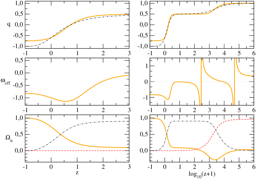
Figure 1: Deceleration $q$, dark energy EOS $\omega_{\rm eff}=p_{\Lambda{\rm eff}}/\rho_{\Lambda{\rm eff}}$, and relative energy densities $\Omega_{n}=\rho_{n}/\rho_{c}$ of dark energy $\rho_{\Lambda{\rm eff}}$ (orange thick curve), dark matter $\rho_{m}$ (black dashed-dotted) and radiation $\rho_{r}$ (red dashed) as functions of redshift $z$ in the model $F=1/B$ with $n=3$, $y=0.7\times 10^{-3}\,H_{0}^{-2/3}$, $\rho_{\Lambda}^{i}=-10^{60}\,\text{GeV}^{4}$, $\Omega_{m}^{0}=0.27$, $\Omega_{r}^{0}=10^{-4}$, $q_{0}\approx-0.6$, $\dot{q}_{0}=-0.5\,H_{0}$. In the deceleration plot the thick orange curve corresponds to the modified gravity model, and the black dashed-dotted curve to $\Lambda$CDM.

It is quite interesting to remark that the EOS analysis suggests that dark energy behaves like dark matter in this epoch, and we will speculate on possible applications in Sec. 5.6. In addition, the tracking relation $\rho_{\Lambda{\rm eff}}\propto\rho_{m}$ reflected in (67) – in which the last two terms on its r.h.s. decay faster than the first and should thus be comparatively negligible – is quite noticeable too, and can be considered as a cornerstone for solving the coincidence problem in the ${\cal F}(R,{\cal G})$-cosmology. Recall that $\rho_{m}=\rho_{m}^{0}\,a^{-3}$ and also that $c_{2}/\rho_{m}^{0}$ need not be a very small number. But even if $c_{2}/\rho_{m}^{0}\simeq 0.1$ the tracking property is remarkable because it shows that the DE and DM densities are following parallel evolutions at different levels, and one is not necessarily infinitesimal as compared to the other. If so, this is an enlightening clue to explain the coincidence problem.

The reason is that when the universe abandons progressively the matter epoch, i.e. when $q$ starts to significantly deviate from $1/2$, then the condition $B\to 0$ is no longer implemented through $q\to 1/2$, but by a significant depletion in the value of the expansion rate itself, which tends to a very small value $H\to H_{*}$ near $H_{0}$. This breaks the approximate “parallel” evolutions of $\rho_{m}$ and $\rho_{\Lambda{\rm eff}}$ (equivalently of $\Omega_{m}$ and $\Omega_{\Lambda{\rm eff}}$) since the universe becomes DE dominated. Thus the two curves must cross (the DE one emerging from below because it was subdominant earlier) and then they meet at some point near our present. This can be seen in the numerical examples presented in Fig. 1 and Fig. 5-8, which sustain our claim that this could be a nice possible explanation for the cosmic coincidence problem. But, even more remarkably, is the fact that it emerges from the same mechanism solving the old CC problem!

5.2 The radiation era

Conventionally, the radiation era is considered as the cosmological time interval which began after the phase of reheating (subsequent to the period of primordial inflation) and ended with the beginning of the matter era, i.e. when $H$ takes values in the range $H_{\rm eq}\leqq H<H_{\rm rad}^{*}$. Accordingly, the deceleration is $q\approx 1$ and $H^{2}\sim\rho_{r}\propto a^{-4}$. Using again the relaxation condition $B\rightarrow 0$ in (62), which in this case amounts to $[H^{2}(1-q)]^{n}\propto H^{4}$, we find

$$R=6H^{2}(1-q)\propto H^{\frac{4}{n}}\propto a^{-\frac{8}{n}}\,.$$ (69)

Note from (53) that the above equation for $H^{2}(1-q)$ will exactly match the scaling behavior $\sim a^{-3}$ of the $\Lambda$CDM model in the matter epoch (for negligible $\rho_{\Lambda}$) only if $n={8}/{3}$. Therefore, we should choose $n$ close to this value to obtain a smooth radiation–matter transition close to the standard model. Equation (53) leads to the relation

$$3H^{2}(1-q)=4\pi G_{N}(\rho_{m}+\rho_{\Lambda{\rm eff}}-3p_{\Lambda{\rm eff}})\propto a^{-\frac{8}{n}},\,\,\,\ \ \ (\rho_{m}=\rho_{m}^{0}a^{-3})\,,$$ (70)

and thus to $p_{\Lambda{\rm eff}}=\frac{1}{3}\rho_{m}+\frac{1}{3}\rho_{\Lambda{\rm eff}}+c_{3}a^{-\frac{8}{n}}$ with $c_{3}=\text{const}$. The dark energy density follows from inserting this expression in the local covariant conservation law (18) and solving it, with the result

$$\rho_{\Lambda{\rm eff}}=c_{4}a^{-4}-\rho_{m}+3c_{3}\left(-4+\frac{8}{n}\right)^{-1}a^{-\frac{8}{n}}\,,$$ (71)

where $c_{4}=\text{const.}$ The corresponding EOS of the effective CC in this epoch interpolates between radiation ($\omega_{\rm eff}\simeq 1/3)$ at early times and dust matter ($\omega_{\rm eff}\simeq 0$) at later times:

$$\omega_{\rm eff}(a)=\frac{p_{\Lambda{\rm eff}}}{\rho_{\Lambda{\rm eff}}}=\left(\frac{1}{3}\right)\,\frac{1+a^{(4-\frac{8}{n})}\frac{3c_{3}}{c_{4}}(1+\left(-4-\frac{8}{n}\right)^{-1})}{1-\frac{\rho_{m}^{0}}{c_{4}}a+a^{(4-\frac{8}{n})}\frac{3c_{3}}{c_{4}}\left(-4+\frac{8}{n}\right)^{-1}}\,.$$ (72)

Also here, a pole in $\omega_{\rm eff}$ might exist depending on $c_{4}$, which can be seen in Fig. 1. Again if $n\gtrsim 2$, the term proportional to $c_{3}$ could lead to an intermediate scaling, which is absent for larger $n$. Remarkably, we find the tracking property $\rho_{\Lambda{\rm eff}}\propto\rho_{r}\propto a^{-4}$ also in the radiation era.

An important point to be stressed in the radiation epoch is that the aforesaid tracking property does not endanger the primordial nucleosynthesis process. In fact, when comparing the scaling law for radiation $\rho_{r}=\rho_{r}^{0}\,a^{-4}$ with equation (71), nucleosynthesis requires that the ratio $c_{4}/\rho_{r}^{0}$ is sufficiently small, typically one order of magnitude at least. We explicitly confirm from the numerical examples in Fig. 1 and Fig. 5-8 that this is indeed the case in the large $z$ region for $z>10^{5}$, which comprises in particular the nucleosynthesis segment around $z\sim 10^{9}$.

The tracking feature of the DE in the matter and radiation epochs, when inspected in Figs. 1 and 5-8, is actually better captured if we focus on the evolution of the EOS parameter as a function of the cosmological redshift, $\omega_{\rm eff}=\omega_{\rm eff}(z)$, rather than looking at e.g. the corresponding behavior of the density parameters $\Omega_{n}$. The point is that, from the figures one might get the wrong perception that $\Omega_{\Lambda{\rm eff}}$ traces $\Omega_{r}$ rather than $\Omega_{m}$ in the matter epoch, and vice versa in the radiation epoch. This is only due to the numerical smallness of $\Omega_{\Lambda{\rm eff}}$ in both the matter and radiation epochs. Instead, when we look at the EOS plots, we see that in the central part of the matter epoch (cf. at the same time the $q$-plot in the interval where $q=1/2$) the EOS of the dark energy tends to stay around $\omega_{\rm eff}(z)\simeq 0$, whereas deep in the radiation epoch ($q=1$) it tends to values around $\omega_{\rm eff}(z)\simeq 1/3$.

For the rest of this work, we want to avoid fractional powers of $n$ in (62) and thus we take the value $n=3$ implying $R\propto H^{\frac{4}{3}}\propto a^{-\frac{8}{3}}$, which is still close to $\Lambda$CDM.

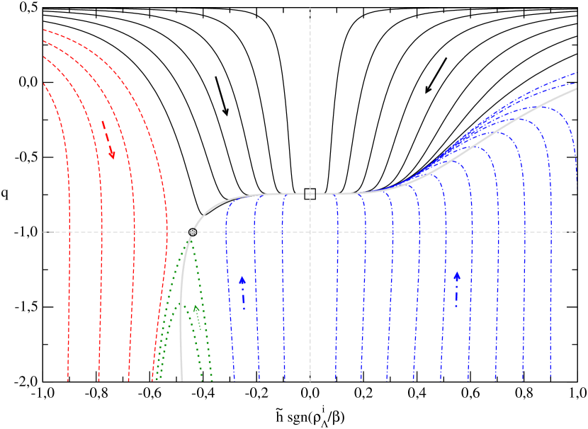
Figure 2: All types of late-time solutions in the $F=1/B$ model as a phase diagram of the deceleration $q$ and the dimensionless Hubble rate $\tilde{h}=\tilde{c}H>0$, $\tilde{c}=|2\rho_{\Lambda}^{i}/\beta|^{1/4}$. The thick grey curve corresponding to $\dot{q}=0$ goes through the unstable de Sitter fixed point at $q=-1$ (circle) and the stable fixed point at $q=a_{1}\simeq-0.74$ (square). The arrows signify the direction of cosmic time.

5.3 The asymptotic late-time evolution

In the previous sections we have analyzed the cosmic evolution in the matter and radiation epochs by making use of $B\rightarrow 0$, i.e. the approximate cancelation of both terms in (62). Accordingly, the behavior of $\rho_{\Lambda{\rm eff}}$ was found without solving the complicated Einstein equations (30). However, in the period from the recent (matter dominated) past to the asymptotic future we cannot profit from the relation $B\rightarrow 0$, because the Hubble rate $H$ is too small making the $y$-term in (62) completely negligible here, so that in good approximation

$$B\simeq\frac{2}{3}R^{2}+\frac{1}{2}{\cal G}=24H^{4}(q-\frac{1}{2})(q-2)\,.$$ (73)

Obviously, the CC relaxation is supported now only by the smallness of $H$, since there are no terms in $B$ which could cancel each other. Before we turn to numerical solutions of the Einstein equations in Sec. 5.4, let us discuss the very late-time evolution analytically, i.e. the asymptotic future regime ($t\to\infty$). For this purpose we consider first the model $F=1/B$ with $y=0$ – i.e. with $B$ given by (73) – and neglect all energy density contributions except for $\rho_{F}$ and $\rho_{\Lambda}^{i}$. This is a good approximation at late times since the Friedmann equation then reads

$$\rho_{c}=\frac{3H^{2}}{8\pi G_{N}}=\rho_{m}+\rho_{\Lambda{\rm eff}}=\rho_{m}+\rho_{\Lambda}^{i}+\rho_{F}\to\rho_{\Lambda}^{i}+\rho_{F}$$ (74)

owing to $\rho_{m}\sim 1/a^{3}\to 0$ for $t\to\infty$. Moreover, the Hubble rate $H$ must be very small in order to sustain the asymptotic late-time relaxation of the effective CC, and hence the effective CC tends to the asymptotically vanishing value of the critical density: $\rho_{\Lambda{\rm eff}}=\rho_{F}+\rho_{\Lambda}^{i}\to\rho_{c}\to 0$. In practice, this means that the equation $\rho_{F}+\rho_{\Lambda}^{i}=0$ should be sufficient for analyzing the background evolution in the asymptotic regime. The induced term corresponding to the $F=1/B$ model can be computed explicitly with the help of (32). After a straightforward calculation, we find

$$\rho_{F}=2\,E_{\,\,0}^{0} = \frac{864\,\beta\,H^{7}}{B^{3}}\left[H(10q^{4}-31q^{3}+15q^{2}+19q-10)-\dot{q}(4q^{2}-10q+7))\right]$$ (75)

$$= \beta\,\left[\frac{5q^{2}-3q-5}{2H^{4}(2q^{2}-5q+2)^{2}}-\frac{\dot{q}\,(4q^{2}-10q+7)}{2H^{5}(2q^{2}-5q+2)^{3}}\right]\,.$$

For the sake of simplifying our discussion below, it is convenient to rewrite the previous equation as follows:

$$\rho_{F}=\beta\left[\frac{k_{1}}{2H^{4}b^{2}}-\frac{\dot{q}}{Hb}\cdot\frac{k_{2}}{2H^{4}b^{2}}\right]\,,$$ (76)

with

$$k_{1} := 5(q-a_{1})(q-a_{2})$$

$$a_{1,2}=\frac{1}{10}\left(3\mp\sqrt{109}\right)$$

$$k_{2} := 4(q-b_{1})(q-b_{2})$$

$$b_{1,2}=\frac{1}{4}\left(5\pm\text{i}\sqrt{3}\right)$$

$$b := 2(q-\frac{1}{2})(q-2)\,.$$

Next, we express the asymptotic Friedmann equation $\rho_{\Lambda}^{i}+\rho_{F}=0$ in terms of a new dimensionless Hubble rate defined as $\tilde{h}:=\tilde{c}H$ and a scaled cosmic time $\tau:=t/\tilde{c}$, where $\tilde{c}:=|x|^{1/4}$ and $x:=\frac{2\rho_{\Lambda}^{i}}{\beta}$, respectively. Denoting $q^{\prime}(\tau)=dq/d\tau$, we have $q^{\prime}(\tau)=\tilde{c}\dot{q}(t)$ and hence Friedmann’s equation can be cast as

$$\mp\tilde{h}^{4}=\frac{k_{1}}{b^{2}}-q^{\prime}(\tau)\frac{k_{2}}{b^{3}\tilde{h}},$$ (78)

where “$-$” corresponds to $x>0$ and “$+$” to $x<0$, respectively. Moreover, the time-evolution of $\tilde{h}$ is the same as that of the true Hubble rate,

$$\tilde{h}^{\prime}(\tau)=-\tilde{h}^{2}(q+1).$$ (79)

From (5.3) and (78) it follows that $q^{\prime}$ and $\tilde{h}^{\prime}$ can be expressed as functions of only $q$ and $\tilde{h}$, which fixes uniquely their evolutions independent of $c$. Instead of plotting a vector map, we show the integrated solutions in Fig. 2, where the arrows indicate the direction of time and the thick grey curve corresponds to $q^{\prime}=0$. In the following we will restrict our analysis to late time solutions $q<\frac{1}{2}$ and $H,\tilde{h}>0$, which implies $b,k_{2}>0$ and $k_{1}\gtrless 0$ for $q\lessgtr a_{1}\approx-0.74$, respectively. Consequently, the deceleration $q$ decreases (becomes more negative) with time on the left-hand side and above of the $q^{\prime}=0$ curve and increases on the right-hand side and below it. Notice from (78) that the de Sitter regime $q=-1$ satisfies $\tilde{h}^{4}=k_{1}/b^{2}=5(1+a_{1})(1+a_{2})/81$, and hence $\tilde{h}=27^{-1/4}$. As the Hubble rate decreases for $q>-1$ and increases for $q<-1$, it follows that the de Sitter fixed point $(q=-1,\tilde{h}=27^{-1/4})$ – see the circle in Fig. 2 – is unstable, and a de Sitter final phase would require fine-tuning. On the other hand, the fixed point $(q=a_{1}\simeq-0.74,\tilde{h}=0)$ – see the square in the central part of Fig. 2 – corresponds to a stable final state similar to quintessence solutions. The red dashed curves describe universes with a decelerating past and a phantom (superaccelerated runaway) future, whereas the black curves approach the stable fixed point with quintessence-like behavior. Also the blue dashed-dotted curves end in the stable fixed point, however they are accelerating in the far past, possibly with a transient decelerating phase in between. Finally, the green dotted curves describe phantom universes with $q<-1$ all the time.

Obviously the most interesting late time solutions obtained from the $F(R,{\cal G})=1/B$ models under study are those showing stable asymptotic quintessence-like behavior. This kind of solutions also exist for more general models, as we shall see below, although the asymptotic future value of the deceleration $q$ will be different in general. Let us look for accelerated solutions with constant $q>-1$ in the asymptotic future (i.e. with a terminal acceleration below the pure de Sitter regime). They correspond to power-law solutions of our field equations in the limit $t\rightarrow\infty$, namely

$$a(t)\propto t^{r}(1+\zeta t^{s})\,,$$ (80)

where a first-order correction $|\zeta t^{s}|\ll 1$ (with $\zeta=\text{const.}$) has been included . We can search for these solutions within the generalized class of models of the form $F(R,{\cal G})=1/B^{m}$ with $m>0$. Obviously, the model we have been considering so far corresponds to the particular case $m=1$. Direct calculations to first order in $\zeta t^{s}$ via (41) and (32) lead to the following results:

$$\rho_{F} = \frac{\beta}{B^{m}}\left(\rho_{F0}+\rho_{F1}\cdot\zeta t^{s}\right)\,,\ \ \ \ \ p_{F}=\frac{\beta}{B^{m}}\left(p_{F0}+p_{F1}\cdot\zeta t^{s}\right)\,,$$ (81)

$$B = 12r^{2}(9r^{2}-9r+2r)t^{-4}+12rs(4-27r+36r^{2}-4s+9rs)t^{-4}\cdot\zeta t^{s},$$

where  $(\rho_{F0}$, $p_{F0})$ and $(\rho_{F1}$, $p_{F1})$ are (dimensionless) time-independent terms corresponding to the zeroth and first order corrections, respectively. In particular,

$$\rho_{F0} = \frac{K(r,m)}{9r^{2}-9r+2}=\left(-1-\frac{4m}{3r}\right)^{-1}p_{F0},$$ (82)

$$K(r,m) = 9r^{2}-9r+2-4m^{2}(9r-4)+3m(3r^{2}-11r+4).$$ (83)

However, these terms are in fact zero because in order to fulfill the late-time Einstein equation $\rho_{F}=-\rho_{\Lambda}^{i}$ we need $K(r,m)=0$, otherwise $\rho_{F}\sim\rho_{F0}B^{-m}\propto t^{4m}$ would diverge for $t\rightarrow\infty$. In addition, we have to fix the correction term in the ansatz (80). This can be achieved by the choice $s=-4m$, as this insures that the term $\rho_{F}\propto\rho_{F1}\cdot\zeta t^{s}B^{-m}\sim t^{s+4m}$ remains essentially constant in time – and this also entails $p_{F}=\text{const}$. Likewise, with this choice of $s$ we have $\zeta t^{s}=\zeta t^{-4m}\to 0$ with increasing $t$ because $m\geq 1$, which means that the correction term in the solution (80) becomes smaller and smaller in the asymptotic regime, irrespective of the particular value of the coefficient $\zeta$. Accordingly, we find

$$\rho_{F1} = \frac{-8m^{2}(4m-1)}{r(9r^{2}-9r+2)^{2}}\,\left[2m^{2}(4-9r)^{2}-3r(7-30r+36r^{2})\right.$$

$$\left.-2m(-8+54r-117r^{2}+81r^{3})\right],$$

$$p_{F1} = \frac{8m^{2}(4m-1)}{3r^{2}(9r^{2}-9r+2)^{2}}\,\left[8+8m^{3}(4-9r)^{2}-72r+171r^{2}-54r^{3}-162r^{4}\right.$$

$$\left.-2m^{2}(-80+408r-585r^{2}+162r^{3})-4m(-16+102r-189r^{2}+54r^{3}+81r^{4})\right],$$

implying

$$\rho_{F1}+p_{F1}=\frac{16m^{2}(4m-1)(2+m(4-9r)-9r+9r^{2})}{3r^{2}(9r^{2}-9r+2)}\cdot\rho_{F0}.$$ (86)

Since the zero-order terms $\rho_{F0}$ and $p_{F0}$ vanish, we obtain the correct asymptotic EOS for the $F$-terms,

$$\omega_{F}=\frac{p_{F}}{\rho_{F}}=\frac{p_{F1}}{\rho_{F1}}=-1\ +\mathcal{O}(\zeta t^{-4m})\,.$$ (87)

It follows that the effective entity that we have called the “cosmon”, and which is responsible for the induced DE – of (modified) gravitational origin – behaves asymptotically as a cosmological term (up to very small corrections). Recall that this is actually so, although in a lesser extent, during most of the cosmological history prior our time. After all the cosmon “duty” is to continually neutralize the initial cosmological term $\rho_{\Lambda}^{i}$ leaving a small dynamical remainder – the measurable CC term. What we have just shown here is that, ultimately, it behaves (very approximately) as a true cosmological constant, with a value equal (but opposite in sign) to the initial CC term: $\rho_{F}(t\to\infty)=-\rho_{\Lambda}^{i}$. Finally, the condition $\rho_{F0}\propto K(r,m)=0$ determines the leading power-law exponent $r$ in the scale factor:

$$r=(6m+6)^{{}^{-1}}(12m^{2}+11m+3\pm\sqrt{144m^{4}+200m^{3}+81m^{2}+10m+1})\,.$$ (88)

Being $r>0$, the evolution law (80) for the scale factor is an increasing one. For $m=1$, we find the solutions $r\approx 0.43$ and $r\approx 3.91$, which are already close to the large $m$ limit solutions $r\rightarrow\frac{4}{9}$ and $r\rightarrow 4m$. Neglecting the correction term, we have $\ddot{a}\sim r(r-1)t^{r-2}$, and hence only the $r>1$ solutions produce acceleration ($\ddot{a}>0$), and only these can be interpreted as asymptotic quintessence-like solutions.

Let us indeed consider in more detail the EOS of the effective vacuum energy $\rho_{\Lambda{\rm eff}}=\rho_{F}+\rho_{\Lambda}^{i}$ in the asymptotic regime. As we know, $\rho_{\Lambda{\rm eff}}$ is essentially zero in this regime, which means that the corresponding EOS function $\omega_{\rm eff}$ cannot be easily derived from the original definition (49) because the latter involves the ratio between the two terms $1+\omega_{F}$ and $\rho_{F}+\rho_{\Lambda}^{i}$ both of which are very close to zero. Let us thus turn to equation (53) and apply it to the very late time epoch, where $\rho_{m}$ can be neglected. It is then easy to show that that equation can be recast in the form

$$\Omega_{\Lambda{\rm eff}}:=\frac{\rho_{\Lambda{\rm eff}}}{\rho_{c}}=\frac{2(1-q)}{1-3\omega_{\rm eff}^{(\infty)}}\,,$$ (89)

where $\omega_{\rm eff}^{(\infty)}$ is the asymptotic value of $\omega_{\rm eff}$. At the same time, we know that in this regime $\rho_{\Lambda{\rm eff}}=\rho_{F}+\rho_{\Lambda}^{i}$ tends to become arbitrarily close to $\rho_{c}$ (both going to zero with the same pace). Thus $\Omega_{\Lambda{\rm eff}}\to 1$, and consequently

$$\omega_{\rm eff}^{(\infty)}=-1+\frac{2}{3}(q+1)\,.$$ (90)

This is the quintessence-like behavior of the EOS for the effective vacuum energy $\rho_{\Lambda{\rm eff}}$ in the asymptotic limit. Notice that since the accelerated expansion implies $\omega_{\rm eff}<-1/3$, we consistently obtain $q<0$. Let us now compute explicitly the deceleration parameter $q$ in the asymptotic regime. Using $q=-1-\dot{H}/H^{2}$ and working out $H=\dot{a}/a$ directly from (80), we find

$$H(t) = \frac{r}{t}\left(1-\frac{4m}{r}\zeta t^{-4m}+{\cal O}(\zeta t^{-4m})^{2}\right)\,,$$ (91)

$$q(t) = -1+\frac{1}{r}+\frac{4m(1-4m)}{r^{2}}\zeta\,t^{-4m}+{\cal O}(\zeta t^{-4m})^{2}\,.$$ (92)

We reconfirm from the last expression that $q<0$ because we look only for the solutions satisfying $r>1$ – the time-dependent term in (92) also respects this feature because $m>1$ and so it contributes negatively. Inserting the previous expression for $q(t)$ in (90) we obtain the asymptotic EOS:

$$\omega_{\rm eff}^{(\infty)}(t)=-1+\frac{2}{3r}+\frac{8m(1-4m)}{3r^{2}}\zeta\,t^{-4m}+{\cal O}(\zeta t^{-4m})^{2}\,.$$ (93)

From this formula, it becomes apparent that the solutions $r>1$ of equation (88) lead to quintessence-like behavior since $\omega_{\rm eff}$ then lies in the interval $-1<\omega_{\rm eff}<-1/3$ (with again a very small time dependence which does not alter this conclusion). Furthermore, if we take e.g. the case $m=1$, equation (88) gives $r\simeq 3.91$ for the $r>1$ solution, and correspondingly equation (92) yields $q\simeq-0.74$ and (93) provides $\omega_{\rm eff}^{(\infty)}\simeq-0.83$ (up to very small time-dependent effects) – see figures 1 and 2. This value of $\omega_{\rm eff}$ can be read directly from Fig. 1 – it corresponds to the value of $\omega_{\rm eff}(z)$ at the terminal point $z=-1$ (i.e. $t\to\infty$).

We may finally derive the very late-time time behavior of $\rho_{\Lambda{\rm eff}}$. As we know, it behaves as $\rho_{\Lambda{\rm eff}}(t)\to\rho_{c}(t)\to 0$ for $t\to\infty$, but we can compute precisely how it decays with time in the last stages of its evolution. Substituting the asymptotic Hubble rate (91) into the asymptotic Friedmann’s equation (74), we arrive at the desired result:

$$\rho_{\Lambda{\rm eff}}=\rho_{\Lambda}^{i}+\rho_{F}=\frac{3}{8\pi G_{N}}\frac{r^{2}}{t^{2}}\left(1-\frac{8m}{r}\zeta t^{-4m}+{\cal O}(\zeta t^{-4m})^{2}\right)\to\frac{3r^{2}}{8\pi G_{N}}\,t^{-2}\ \ \ (t\to\infty)\,,$$ (94)

where $m\geq 1$ for all the relaxation models under consideration. Let us also note (a posteriori) that the obtained result is consistent with our assumption that the asymptotic matter density decays always faster than the vacuum energy density, as we supposed from the very beginning in (74). Indeed, being $\rho_{m}\sim a^{-3}\sim t^{-3r}$ – where we can neglect here the small correction term in (80) – the matter density is always much smaller than the effective vacuum energy $\rho_{\Lambda{\rm eff}}\sim t^{-2}$ because the minimum value of $r$ (for accelerating solutions) is approximately $r\simeq 3.91$, which is attained for $m=1$ – cf. equation (88). For $m>1$, $r$ is larger than the previous value and the desired condition is always secured.

Looking at the numerical examples presented in Figs. 1 and 5-8, we can check that the asymptotic $t\to\infty$ (i.e. $z\to-1$) EOS behavior $\omega_{\rm eff}=\omega_{\rm eff}(z)$ of the effective CC is always quintessence-like ($-1<\omega_{\rm eff}<-1/3$). However, in some cases (e.g. in Figs. 1 and 5), it presents an effective phantom phase $\omega_{\rm eff}<-1$ for non-asymptotic regions, actually for regions not far away in our past. Therefore, the accessible region to our observations could present an effective phantom-like DE behavior. In contradistinction to scalar models of the DE, this phantom-like behavior has nothing to do with negative kinetic terms, as it is of purely effective nature. For example, since $\Omega_{\rm eff}(z)>0$ in the affected regions of Figs. 1 and 5, the phantom behavior is just triggered by the fact that the set of terms in the field equations that we have collected under the name of the cosmon produces $(1+\omega_{F}(z))\rho_{F}(z)<0$ in those redshift segments – cf. equation (49).

5.4 Parameters and initial conditions

Our modified gravity action (22) with $F=1/B$ or more generally $F=R^{s}/B^{m}$ contains two parameters $\beta$ and $y$, where the latter is directly related to the radiation-matter transition. To solve the Einstein equations, we have to impose one more initial condition because $F(R,{\cal G})$ theories have more degrees of freedom than general relativity. In fact, while in the standard $\Lambda$CDM model the initial value of the deceleration $q_{0}$ is fixed simply by the current relative densities $\Omega_{n}^{0}$, see equation (54) (specifically $q_{0}=\Omega_{m}^{0}/2-\Omega_{\Lambda}^{0}$ for the present epoch), in the relaxation model we have to provide also the value of $\dot{q}_{0}$. To see this, note that the induced $F$-term is a function of the type

$$\rho_{F}=\rho_{F}(H,q,\dot{q};\beta,n,y)\,,$$ (95)

which depends in general on the three free parameters (64) and involves $H$, $q$ and also $\dot{q}$. Recall that $n=3$ was fixed because it provides a sufficiently smooth transition from the radiation to the matter epochs, so only $\beta$ and $y$ remain as free parameters to be chosen. An explicit example is the late time form given in equation (75), where the $\dot{q}$ dependence is manifest. Therefore, if we are given $\rho_{\Lambda}^{i}$ and we fix the current value of the CC density, this amounts to fix the value of

$$\Omega_{\Lambda{\rm eff}}^{0}=\frac{\rho_{\Lambda}^{i}+\rho_{F}(H_{0},q_{0},\dot{q}_{0};\,\beta,n,y)}{\rho_{c}^{0}}\,,$$ (96)

which entails a non-trivial relation between the parameters. This relation involves explicitly the value of $\dot{q}_{0}$, and in our case $q_{0}$ is fixed from equation (55). Therefore, equation (96) fixes $\dot{q}_{0}$, which is tantamount to say that $\dot{q}_{0}$ must be provided as an additional input in order that the value of the current $\Omega_{\Lambda{\rm eff}}^{0}$ is correctly matched.

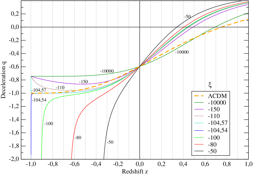
Figure 3: Possible future final states in the class of $F=1/B$ models. Shown is the deceleration parameter versus redshift for different values of the dimensionless parameter $\xi=3\beta/(\rho_{\Lambda}^{i}\,H_{0}^{4})$, assuming $\xi<0$ in all cases. Depending on the value of $|\xi|$, in the asymptotic limit $t\to\infty$ (i.e. $z\to-1$) the universe expands approximately according to a power-law $a\sim t^{r}$ ($r\simeq 3.91$ for this class of models) or else it develops a future singularity characterized by a runaway acceleration ($q\ll-1$). Notice that de Sitter space-time ($q=-1$) lies on the boundary between the two possibilities.

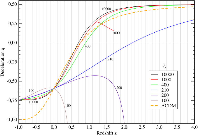
Figure 4: As in Fig. 3, but for $\xi>0$. Notice that here all curves have an asymptotic power-law expansion  $a(t)\sim t^{r}$ for $t\rightarrow\infty$. However, not all curves are admissible since $\xi$ is limited from below ($\xi\gtrsim 210$) in order to have a matter era ($q\approx\frac{1}{2}$) in the past.

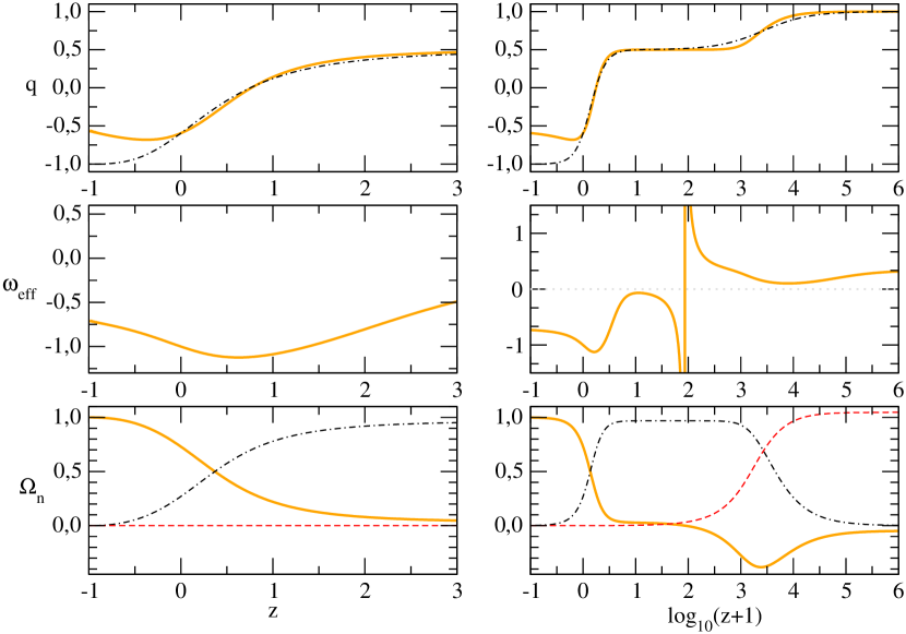
Figure 5: Model $F=R/B$ with $n=3$, $y=0.7\times 10^{-3}\,H_{0}^{-2/3}$, $\rho_{\Lambda}^{i}=-10^{60}\,\text{GeV}^{4}$, $\Omega_{m}^{0}=0.27$, $\Omega_{r}^{0}=10^{-4}$, $q_{0}\approx-0.6$, $\dot{q}_{0}=-0.5\,H_{0}$. The curves have the same meaning as in Fig. 1.

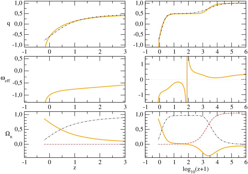
Figure 6: Model $F=R^{2}/B$ with $n=3$, $y=0.7\times 10^{-3}\,H_{0}^{-2/3}$, $\rho_{\Lambda}^{i}=-10^{60}\,\text{GeV}^{4}$, $\Omega_{m}^{0}=0.27$, $\Omega_{r}^{0}=10^{-4}$, $q_{0}\approx-0.6$, $\dot{q}_{0}=-1.8\,H_{0}$. There is a future singularity at $z>-1$. The curves have the same meaning as in Fig. 1.

For definiteness, let us now focus for a while on the canonical type of models characterized by $F=1/B$, i.e. our starting class of models defined in section 3.2. As we know, for these models $\beta$ has mass dimension 8 and can be represented as $\beta\equiv{\cal M}^{8}$, with ${\cal M}$ some mass scale. This suggests that the numerical analysis of the $F=1/B$ models can be more conveniently performed using the dimensionless combination $\xi\equiv 6/(x\,H_{0}^{4})=3\beta/(\rho_{\Lambda}^{i}\,H_{0}^{4})$ as an input parameter. In Figs. 3 ($\xi<0$) and 4 ($\xi>0$), we plot the deceleration $q$ for different values and signs of $\xi$ (or equivalently of $\dot{q}_{0}$). In these examples we use $q_{0}\simeq-0.6$ for the current deceleration, although one has some freedom here, too. The plots show a broad range of different solutions for $q$, with some of them close to the $\Lambda$CDM evolution. Remember that the latter makes a precise prediction for the transition redshift from deceleration to acceleration, given by

$$z^{*}=-1+\sqrt[3]{2\,\frac{\Omega_{\Lambda}^{0}}{\Omega_{m}^{0}}}\simeq 0.75\,,$$ (97)

where the numerical value corresponds to our choice $\Omega_{m}^{0}=0.27$ (hence $\Omega_{\Lambda}^{0}=0.73$ for a flat universe). We see that most of the examples plotted in Fig. 3 – corresponding to different values of the parameter $\xi$ and the initial conditions as in Fig. 1 – predict a transition redshift smaller and hence nearer to our time, meaning that the accelerated expansion is more recent. For large and negative $\xi$, however, one finds $z^{*}\simeq 0.7$ and the $\Lambda$CDM result can almost be matched – see e.g. the $\xi=-10^{4}$ curve in Fig. 3. In this example, if we take as usual $|\rho_{\Lambda}^{i}|\sim M_{X}^{4}$ with $M_{X}\sim 10^{16}$ GeV, and we recall that $H_{0}\sim 10^{-42}\,\text{GeV}$, we find ${\cal M}=\beta^{1/8}\sim 10^{-4}$ eV, i.e. a mass scale characteristic of light neutrinos. Similarly in Fig. 4, corresponding to $\xi>0$, although in this case we can see that there are values that give a transition redshift much earlier in time (i.e. a more remote onset of the acceleration period), although the scale ${\cal M}$ remains of the same order of magnitude. In fact, all values of $|\xi|$ in the wide interval $1\lesssim|\xi|\lesssim 10^{8}$ render ${\cal M}$ in the light neutrino range $10^{-4}\,\text{eV}\lesssim{\cal M}\lesssim 10^{-3}$ eV. However, for $\xi>0$ the values which are below $210$ are clearly excluded as they correspond to $q<0$ in the past and therefore the matter epoch ($q=1/2$) would not have occurred.

A few more observations are worthwhile in regard to Figs. 3 and 4. For negative values of $\xi$, the asymptotic evolution follows either the power-law expansion discussed above (if $|\xi|\gtrsim 105$) or a future singularity (if $|\xi|<104$). This singularity corresponds to a situation leading to superaccelerated cosmology ($q\ll-1$) ending in a Big Rip. The boundary between both final states is de Sitter space-time ($q=-1$). Larger values of $|\xi|$ lead to an expansion behavior quite close to $\Lambda$CDM in the recent past. In the case of positive $\xi$, only the power-law solution exists for $t\rightarrow\infty$. However, as already mentioned, in this case $|\xi|$ is bounded from below. Summarizing, late-time expansion histories close to $\Lambda$CDM (as suggested by observations) require large values of the parameter $|\xi|$ (hence of $\beta$, for a given $\rho_{\Lambda}^{i}$), which always imply a power-law future state. In the limit $|\beta|\rightarrow\infty$ we find for both signs of $\rho_{\Lambda}^{i}$ the value $\dot{q}_{0}\approx-0.57\,H_{0}$, and the evolution of $q$ becomes very insensitive with respect to $\beta$, see Fig. 4. The last statement can be derived from (75), where we see that the terms in square brackets must vanish for $|\beta|\rightarrow\infty$, otherwise the Einstein equation (50) is not fulfilled. Consequently, $\dot{q}$ does not depend on $\beta$ since it can be expressed as a function of $q$ and $H$ only.

The phantom universes with $q<-1$ at all times (green dotted curves in Fig. 2) are not among the numerical solutions since we fixed the initial conditions to $q_{0}=-0.6$. This also explains the absence of the solutions plotted as blue dashed-dotted curves in the case $\xi<0$. Finally, let us also remark that although the numerical examples displayed in Figs. 1 and 5-8 correspond to $\rho_{\Lambda}^{i}<0$ (basically because, as we have discussed in section 2, this is the situation in the important case of the SM of particle physics), a similar set of relaxation curves would be obtained for $\rho_{\Lambda}^{i}>0$.

5.5 Generalized relaxation models: $F^{s}_{m}=R^{s}/B^{m}$ and beyond

Without much effort the results in Sec. 4.2 can be carried over to many models which have a factor $B^{-1}$ in $\rho_{\Lambda{\rm eff}}$ and $p_{\Lambda{\rm eff}}$. The natural generalization is to consider models of the form

$$F^{s}_{m}:=\frac{R^{s}}{B^{m}}=\frac{R^{s}}{\left[\frac{2}{3}R^{2}+\frac{1}{2}{\cal G}+(y\,R)^{n}\right]^{m}}\,,\ \ \ \ (s\geq 0,m>0;\,n>2)\,.$$ (98)

Recall that we usually choose $n=3$ to smooth the transition between radiation and matter eras. The canonical model with which we have started in section 3.2 is just the particular case $F^{0}_{1}$, and the models considered in equation (81) are the $F^{0}_{m}$ ones. The cosmic evolution of $q(z)$ in the matter and radiation epochs for $F^{s}_{m}$ does not show any relevant differences with respect to $F^{0}_{1}$ because only the structure of $B$ is important there, in the sense that the relaxation relation $B\rightarrow 0$ holds. However, the relative energy densities $\Omega_{n}(z)$ of the matter/energy components and the EOS $\omega_{\rm eff}$ may evolve differently, which is demonstrated in Figs. 5, 6 and 7. Moreover, at late times also the deceleration $q$ may differ significantly among the models.

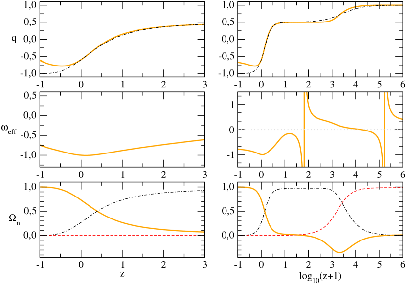
Figure 7: Model $F=R^{3}/B^{2}$ with $n=3$, $y=0.75\times 10^{-3}\,H_{0}^{-2/3}$, $\rho_{\Lambda}^{i}=-10^{60}\,\text{GeV}^{4}$, $\Omega_{m}^{0}=0.27$, $\Omega_{r}^{0}=10^{-4}$, $q_{0}\approx-0.6$, $\dot{q}_{0}=-0.8\,H_{0}$. The curves have the same meaning as in Fig. 1.

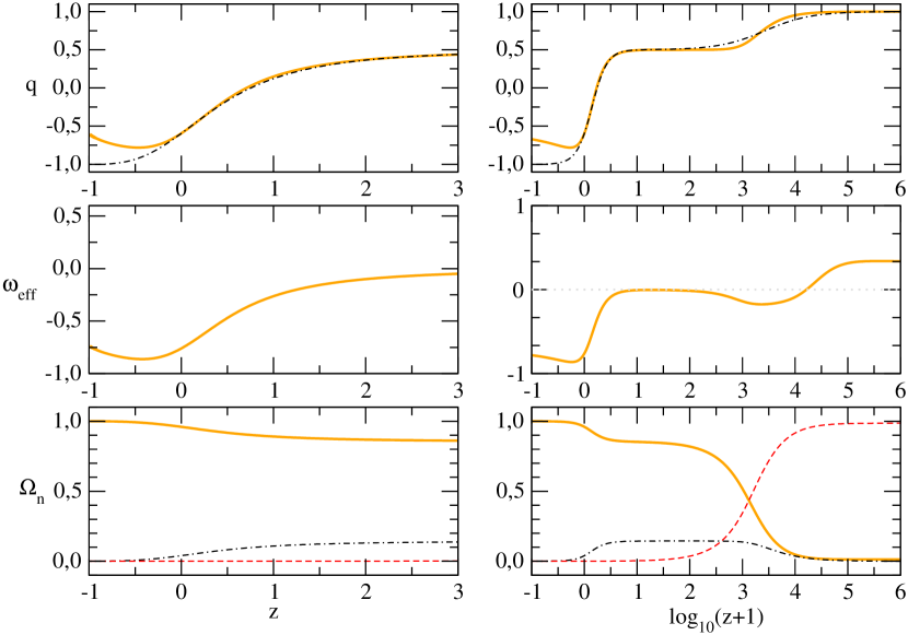
Figure 8: The unified dark matter/dark energy scenario from Sec. 5.6 in the model $F=R^{3}/B^{2}$ with $n=3$, $y=0.75\times 10^{-3}\,H_{0}^{-2/3}$, $\rho_{\Lambda}^{i}=-10^{60}\,\text{GeV}^{4}$, $\Omega_{m}^{0}=0.04$, $\Omega_{r}^{0}=10^{-4}$, $q_{0}\approx-0.6$, $\dot{q}_{0}=-0.8\,H_{0}$. The curves have the same meaning as in Fig. 1 except for $\Omega_{m}^{0}$ (black dashed-dotted), which represents the baryons only. The unified dark component exhibits a positive energy density $\rho_{\Lambda{\rm eff}}>0$ at all times.

Apart from dynamical properties, the dimensionality and the value of the parameter $\beta$ depend on the particular generalized class $F^{s}_{m}$ of $F(R,{\cal G})$ functional, too. One can easily show that the parameter $\beta$ is related to a power of a mass scale $M$ as

$$|\beta|=M^{4-2s+4m}\,.$$ (99)

All these models yield induced DE terms of the form $\rho_{F},p_{F}\propto B^{-p}$ with $p>0$ as a result of equations (32) and (33), where the derivatives of $F$ and ${\cal G}$ introduce more factors of $B$ in the denominators. One can readily show that the CC relaxation and tracking properties in the matter and radiation eras follow again from the relaxation condition.

For estimating $\beta$ let us assume that each time derivative in the expression for $E_{\,\,0}^{0}$ – see equation (32) – yields a factor $H_{0}$ today, and no accidental cancelations are present so that $B\sim H_{0}^{4}$. Consequently, in the model $F^{0}_{1}=1/B$, we find $\rho_{F}^{0}\sim\beta/H_{0}^{4}$ for the current value of the induced term, as in the toy model example of section 4.1. Indeed, in the late epoch, where $q$ ceases to play a significant role, the realistic model based on (62) produces qualitatively the same picture as in the simple one (59). Therefore, within one order of magnitude, equation (61) holds again and we can estimate the value of the parameter $\beta$ using the current value of the Hubble rate, $H_{0}\sim 10^{-33}$ eV. Since $\rho_{F}^{0}\sim-\rho_{\Lambda}^{i}$ and $|\rho_{\Lambda}^{i}|\sim M_{X}^{4}$, we get

$$|\beta|\equiv{\cal M}^{8}\sim|\rho_{F}^{0}|\,H_{0}^{4}\sim M_{X}^{4}\,H_{0}^{4}\,,$$ (100)

where $\beta$ is expressed as a power of an energy scale ${\cal M}$ as in (27). Taking the standard GUT scale $M_{X}\sim 10^{16}$ GeV, we obtain once more a mass value for ${\cal M}$ of the order of a light neutrino mass:

$${\cal M}\sim\sqrt{M_{X}\,H_{0}}\sim 10^{-4}\,\text{eV}\,.$$ (101)

Incidentally, this value for $M$ is the geometric mean of the two most extreme mass scales available in our universe below the Planck mass. Such value is by the way not far from the mass scale associated to the current value of the CC: $m_{\Lambda}\equiv\left(\rho_{\Lambda}^{0}\right)^{1/4}\sim 10^{-3}$ eV, and it should therefore be considered quite natural. Actually, the value of ${\cal M}$ obtained in a given model could be larger than our rough estimation, especially if cancelations in $E_{\,\,0}^{0}$ occur, but as we shall see there is a wide spectrum of possible values for ${\cal M}$ in the class of $F^{s}_{m}$ models, and all of them within a reasonable particle physics range.

In fact, applying the same arguments for the models $F^{1}_{1}=R/B$ and $F^{3}_{2}=R^{3}/B^{2}$ we find in both cases $|\beta|={\cal M}^{6}\sim\rho_{\Lambda}^{i}\,H_{0}^{2}\sim M_{X}^{4}\,H_{0}^{2}$, which implies ${\cal M}\sim 0.1\,\text{GeV}$. This is again a reasonable mass scale in particle physics, as it is of the order of the characteristic QCD scale of the strong interactions, ${\cal M}\sim\Lambda_{QCD}\simeq 100$ MeV. Finally, the model $F^{2}_{1}=R^{2}/B$ yields $|\beta|={\cal M}^{4}=|\rho_{\Lambda}^{i}|\sim M_{X}^{4}$, and in this case ${\cal M}$ would be close to the initial vacuum energy scale $M_{X}$ of the GUT . This situation is also perfectly reasonable inasmuch as $M_{X}$ is another natural scale of the problem, just the one placed at the starting point of the evolution. Remarkably, the mass parameter $M$ of the relaxation mechanism is not only completely free from fine-tuning problems, it also lies in a perfectly reasonable range of particle physics masses, possibly related to neutrinos, QCD or even GUT models. In all these situations the relaxation mechanism takes care automatically that the observable CC scale of the vacuum energy density is $\rho_{\Lambda{\rm eff}}(H)\sim\rho_{\Lambda}^{0}$ at $H=H_{0}$.

In summary, the energy scale ${\cal M}$ of the CC relaxation mechanism could be very well related to reasonable mass scales in Particle Physics, thereby avoiding tiny energy scales $H_{0}\sim 10^{-33}$ eV which so often appear in many dark energy models (for example, in quintessence models [13]). Once the correct $F$-term has been identified, the mass scale ${\cal M}$ should be considered a sort of “constant of Nature”, and in this sense we expect it should bear direct relation with a particle physics scale of the SM or of a typical GUT scale.

We remark that the fact that the initial cosmological term $\rho_{\Lambda}^{i}$ was considered constant (but otherwise arbitrary), is not a real limitation for the efficiency of our dynamical adjustment mechanism. This mechanism works for virtually any cosmological model in the general class of $\Lambda$XCDM models [24, 25]. In particular, we cannot exclude that the initial vacuum energy density can be evolving with time through some cosmological quantity $\xi=\xi(t)$, i.e. $\rho_{\Lambda}=\rho_{\Lambda}(\xi(t))$. For example, it has been suggested in the literature that $\rho_{\Lambda}$ could be a quadratic function of the expansion rate: $\rho_{\Lambda}(H(t))=n_{0}+n_{2}\,H^{2}(t)$, where $n_{0}$ and $n_{2}$ are both non-vanishing coefficients, see e.g. the recent papers [14, 15, 33] and the older ones [16, 17]. The reason for this “running” of the vacuum energy stems from the expanding background, and these papers suggested that the quantum effects provide precisely this running behavior. For a summary of alternative proposals of evolving vacuum energy that have recently been tested in the light of the most recent cosmological data, see e.g. [22].

In the present framework, the effective vacuum energy $\rho_{\Lambda{\rm eff}}$ is anyway a mildly evolving quantity, even in the absence of the aforementioned running contributions. But if one accepts that the running terms are also there, nothing essential is changed in our relaxation mechanism. One has to keep $\dot{\rho}_{\Lambda}\neq 0$ in the covariant conservation law (20) and the $F$-functional will adjust automatically the contribution of the additional terms. Technically, however, let us clarify that if these contributions are added directly at the level of the field equations, then in order to keep matter conservation we have to allow for a “running gravitational coupling $G_{N}$” as well. This possibility has also been contemplated in the literature and it corresponds to the so-called type-II $\Lambda$XCDM models [25], in which the energy density conservation law involves $\dot{\rho}_{\Lambda}\neq 0$ and $\dot{G}_{N}\neq 0$ simultaneously. We refer the reader to the aforesaid reference for details.

Finally there is still another modification of our relaxation functional that may be necessary in order to make our cosmological model a bit more realistic: we have to insure that the modified gravitational action (22), once it is written in a metric amenable for Solar System tests (namely, the Schwarzschild metric in the presence of a cosmological term), is able to pass these tests and at the same time keeps its ability to reduce dynamically the value of the cosmological constant within observations. While a detailed treatment of this problem will be presented elsewhere [57], in Appendix C we briefly describe the kind of modification that we have to introduce on the functional ${\cal F}$ such that it fulfills all these requirements without altering in any essential way the dynamical relaxation mechanism that we have studied so far.

5.6 Special scenario: unified dark matter and dark energy

In this section we discuss a special scenario of unified dark matter and dark energy. At least for the background evolution this seems to be possible because the dark energy density $\rho_{\Lambda{\rm eff}}$ behaves like dust matter in the matter era, see equation (67). Therefore, it might replace dark matter completely. Whether the effective dark energy/matter in our setup provides the correct clustering properties to successfully seed structure formation will be studied in a future work together with its evolution on solar system and galactic scales . If it works, we would find a MOND-like theory since our modified gravity model had to simulate the effect of standard dark matter.

In the following, we concentrate on the cosmic background expansion. The model shown in Fig. 8 describes a universe with only baryons $\Omega_{m}^{0}=0.04$, dark energy and radiation $\Omega_{r}^{0}=10^{-4}$. Since standard dark matter is absent, the relative energy densities of dark energy and the baryons sum up to unity in the matter era. At late times and during the radiation epoch there is no big difference between this special relaxation scenario and the previously studied relaxation models with dark matter.

Finally, we mention two advantages of this approach. First, we do not need the parameters related to dark matter ($\Omega_{dm}^{0}$) because $y$ fixes the radiation–matter transition. Second, it is possible to have $\rho_{\Lambda{\rm eff}}>0$ all the time, which leads to an effective EOS for $\rho_{\Lambda{\rm eff}}$ without spurious divergences. In fact, these divergences should not represent a real problem, they just indicate that $E_{\,\,0}^{0}$ in (32) vanishes. However, in this special scenario the full ${}_{\,\,0}^{0}$-component in the Einstein equation remains always positive.

6 Conclusions

In this work, we have made a thorough attempt to deal with the old cosmological constant (CC) problem [3] – the toughest cosmological conundrum of all times. It suggests that our vacuum should contain a huge energy density $\rho_{\Lambda}^{i}$ coming from quantum zero-point energies and phase transitions in the early universe. This formidable problem cannot be solved by just finding a source for the late-time acceleration of our cosmos. Instead, it requires a powerful mechanism capable of disarming the large CC during all known stages of the cosmological evolution, not just at the last stages. Scalar field models, for instance, completely fail to solve the old CC problem, as they actually introduce two severe theoretical diseases: 1) extreme fine-tuning of the parameters (through e.g. an ad hoc counterterm in the potential that cancels the initial CC), and 2) an extremely tiny mass scale needed to match the ground state potential with the present value of the CC. Such mass scale is usually as small as $H_{0}\sim 10^{-33}$ eV, i.e., very many orders of magnitude smaller than the natural mass scale $m_{\Lambda}\equiv(\rho_{\Lambda}^{0})^{1/4}\sim 10^{-3}$ eV associated to the observationally measured value of the vacuum energy density. Quintessence models, therefore, do not really solve the problem since they input two highly unnatural ingredients that completely spoil the credibility of the proposal. If that is not enough, they simply put the vacuum energy under the rug as if it would not exist, and then focus exclusively on the special properties of the newly invented scalar field.

Clearly, a radically different new approach is required. In an attempt to make a first step in this direction, we have proposed a self-adapting (dynamical) relaxation mechanism based on a pure modification of gravity. Thanks to it, we can avoid fine-tuning at all stages of the cosmological evolution. More specifically, we have demonstrated that an arbitrarily large initial CC can be relaxed automatically by complementing the Einstein-Hilbert action with a class of action functionals of the Ricci scalar and the Gauß-Bonnet invariant, ${\cal F}(R,{\cal G})$. The two most remarkable achievements of our relaxation mechanism is the complete absence of fine-tuning in the parameters of the model, and at the same time the absence of tiny mass scales. The modified gravity action induces a dynamical dark energy component, $\rho_{F}$, associated to the ${\cal F}$-functional. This induced DE density acts effectively as a “dynamical counterterm”, i.e. one that self-adjusts to the necessities of the universe at any given moment, and is able to efficiently neutralize any exceedingly large vacuum energy $\rho_{\Lambda}^{i}$ left over near the radiation epoch by the primeval inflation mechanism, thus preventing the universe from the disastrous effects that would ensue otherwise (as e.g. the disruption of the primordial nucleosynthesis epoch). Indeed, by becoming sufficiently large to compensate for the initial CC, the effective energy density $\rho_{F}$ generated by the ${\cal F}$-functional self-adapts automatically to the initial conditions of the universe and to the subsequent radiation and matter epochs, and enforces the universe to follow the standard FLRW cosmic expansion history in each one of these epochs.

As a result, the “residual” dark energy of our model (or effective vacuum energy density $\rho_{\Lambda{\rm eff}}$) appears, at every stage of the cosmological evolution, as a mildly evolving function of the expansion rate, $\rho_{\Lambda{\rm eff}}(H)=\rho_{\Lambda}^{i}+\rho_{F}(H)$. This function takes values much smaller than the initial $\rho_{\Lambda}^{i}$ because there is a large (and automatic) compensation of it with the values taken by $\rho_{F}(H)$, which have opposite sign. Moreover, $|\rho_{\Lambda{\rm eff}}(H)|\ll|\rho_{\Lambda}^{i}|$ holds good for all values of $H$ at (and below) the radiation epoch, and for any given $\rho_{\Lambda}^{i}$. In addition, the current value of $\rho_{\Lambda{\rm eff}}$ can be of the order of the measured one by the modern cosmological data, i.e. $\rho_{\Lambda{\rm eff}}^{0}\equiv\rho_{\Lambda{\rm eff}}(H=H_{0})\simeq\rho_{\Lambda}^{0}\simeq 10^{-47}\,\text{GeV}^{4}$, without introducing fine-tuning or any unnaturally small parameter. In fact, the small $\rho_{\Lambda{\rm eff}}^{0}$ is the observable cosmological term in the present framework, whereas the large initial CC value $\rho_{\Lambda}^{i}$ (and the corresponding dynamical counterterm $\rho_{F}$) cannot be resolved individually from the usual CC measurements.

All in all, our model – the Relaxed Universe – appears very similar to the standard Big Bang model and resembles the late universe near our time (concordance $\Lambda$CDM model) in most respects, irrespective of the initial vacuum conditions. Therefore, the ${\cal F}(R,{\cal G})$-cosmology appears all the time as a FLRW model with essentially constant and tiny cosmological term. In addition, the vacuum energy $\rho_{\Lambda{\rm eff}}$ exhibits remarkable tracking properties because it evolves like radiation or dust matter in the corresponding cosmological epochs. This feature of the model sheds considerable light also on the cosmic coincidence problem inasmuch as it provides a raison d’être for the fact that the DE and DM densities are still close at present. Indeed, one finds that the DE and DM were cosmic companions with similar EOS and approximately proportional densities, and this was so all the time until very recently, namely until the matter epoch extinguished (meaning that $q$ departed much from $1/2$) and the universe – which is constantly fueled with the big initial $\rho_{\Lambda}^{i}$ – was forced to use the last resort of the relaxation mechanism available under these circumstances, which is to take a very low value of $H$ in order to compensate for $\rho_{\Lambda}^{i}$ and still keep showing a small observable $\rho_{\Lambda{\rm eff}}$. That crucial event decoupled once and forever the tracking behaviors of matter/radiation and DE, and since then the DE dominates the universe expansion. Such breakdown of the tracking property at the end of the matter epoch, on the other hand, pushed the subdominant DE density curve upwards until crossing the decaying DM one at some point after the matter epoch and hence near our time. This is the origin of the “coincidence” event in our late time neighborhood. But, most remarkable of all, the primary trigger of this crossing event (representing the startup of the DE era) is the relaxation mechanism itself, which is therefore simultaneously responsible for explaining – and linking together – the two fundamental CC conundrums of our current Cosmos: the old CC problem and the cosmic coincidence problem.

Worth noticing is also the fact that the asymptotic late time behavior of the universe in the DE epoch mimics the quintessential or phantom behavior. Only under special initial conditions, the future behavior can be de Sitter space-time, but any perturbation of these conditions would tilt its evolution into one of the aforementioned forms.

The dynamical solution found in this paper resembles, in a sense, the one so longed for by scalar field model builders, except that these kind of models always failed because they ultimately involve fine-tuning (as proven by the famous Weinberg’s no-go theorem [3]). Even if the ${\cal F}(R,{\cal G})$-cosmology lacks at the moment of a fundamental understanding of the origin of the ${\cal F}$-functional, the situation is not very different from the innumerable and unsuccessful attempts based on scalar field models where one has no fundamental motivation for using a particular potential that serves our purposes. The advantage of the ${\cal F}(R,{\cal G})$-cosmology, in contrast, is that the job is done by gravity itself, and is done correctly, namely without fine-tuning inconsistencies. This was never achieved with scalar field models nor with any other cosmological model that we know of.

In its current stage, we have been able to devise a relaxation mechanism which starts working automatically in the early radiation dominated epoch, hence right after the reheating process that follows primordial inflation. It was not our purpose here to identify the fundamental physics that may have triggered this mechanism. It could have been caused by an “effective inflaton” reaching the minimum of its potential, especially if the minimum lies below zero and having an arbitrary value $|\rho_{\Lambda}^{i}|$. This value fixes the initial (usually large) CC of the universe just before starting the radiation epoch. The latter case appears much more likely than just assuming (as usually done in the literature) that the inflaton potential has been fine-tuned to almost vanishing ground state energy at the radiation epoch. Furthermore, since our relaxation ${\cal F}$-functional is constructed from a modified gravity theory, it is natural to complement it with the standard $R^{2}$ terms of the renormalizable effective action of gravity. These terms do not alter the relaxation mechanism in any significant way, as we have seen, but they can just take care of the UV behavior of the theory and even be responsible for inflation itself.

In the framework of modified gravity, the successful relaxation of the CC requires an action functional ${\cal F}(R,{\cal G})$ with a special structure, namely one which leads to an induced dark energy density being able to compensate dynamically the initial CC. However, our approach is not limited to a very specific model of this kind; actually, a whole class of working relaxation models $F^{s}_{m}$ has been uncovered. On the basis of several analytical and exact numerical examples, we have shown that they differ mostly at late times in accordance with the requirement of the current cosmos being close to $\Lambda$CDM. Interestingly enough, our action functional ${\cal F}$ contains a mass scale ${\cal M}$ whose natural value can either be a typical particle physics mass of the standard model of strong and electroweak interactions (say, a neutrino mass, the QCD scale etc) or even a typical Grand Unified mass $M_{X}$. But ${\cal M}$ is never an extremely tiny mass scale of order of $H_{0}\sim 10^{-33}$ eV, which so often appears in the DE models of the literature. In summary, we can say that the typical values for the fundamental mass scale ${\cal M}$ that are needed to solve the CC fine tuning problem in our framework range from the present CC mass scale, $m_{\Lambda}\equiv\left(\rho_{\Lambda}^{0}\right)^{1/4}\sim 10^{-3}$ eV, to the value of the initial CC mass scale, $\left(\rho_{\Lambda}^{i}\right)^{1/4}\sim M_{X}\sim 10^{16}$ GeV. What else could be more natural?

The model universe we have envisaged here falls within the general class of the $\Lambda$XCDM models of the cosmic evolution [24, 25, 26], in which a new entity $X$ (the “cosmon”) appears in interplay with the cosmological term. Such an entity is in general not a field, but a complicated effective quantity. The cosmon is in fact associated here to the induced DE density $\rho_{F}$ which is generated from the ${\cal F}$-functional at the level of the field equations. While in Ref. [24] the cosmon served the main purpose of solving (or highly palliating) the cosmic coincidence problem, here the cosmon is eventually responsible for solving the fine-tuning CC problem, and hence it provides a first fundamental step towards solving (or highly alleviating) the old CC problem. Amazingly enough, it provides a clue for solving the coincidence problem as well, as we have seen. Therefore, while in the present realization the cosmon does not appear as an elementary particle, it does however fully accomplish its main aim, which is to cure the CC fine-tuning problem. Let us recall that the name “cosmon” was coined for the first time in the literature in Ref. [51], and in its first implementation it was a scalar field, hence afflicted by the aforementioned Weinberg’s no-go theorem. In the modern version, it is not. Therefore, the new cosmon well deserves its name, for it fully adapts to the original sense of the old literature as being an entity which is able to dynamically adjust the value of the cosmological constant [51]. The cosmon, indeed, generates the dynamical counterterm $\rho_{F}$ which is able to continuously neutralize the very large $|\rho_{\Lambda}^{i}|\sim M_{X}^{4}$ in all epochs of the post-inflationary cosmic evolution.

In summary, in this paper we have extensively discussed the working principle of the relaxation mechanism and the corresponding background evolution of the ${\cal F}(R,{\cal G})$ cosmology. In doing this we have found an exceptional model universe, the Relaxed Universe, in which all the main tensions with the observational data are relaxed and can be smoothly accommodated in its inner dynamics. The Relaxed Universe seems to be a promising candidate for our real universe since it is essentially free from the toughest cosmological puzzles, the old CC problem and the cosmic coincidence problem. Its explicit construction constitutes a “proof of existence” of a dynamical mechanism that may account for the value of the current cosmological constant, starting from a value of arbitrary size. However, although our results are very encouraging, this is just one more step in the right direction. More efforts are necessary to uncover all the main properties of our model and resolve upcoming problems. In the future, we plan to investigate further aspects of this setup, e.g. the evolution of perturbations, the Newtonian limit and possible instabilities, leading to new insights and improvements. Also, it will be interesting to know if the unification of dark matter and dark energy can be fully realized in this framework. And of course one should eventually look for a fundamental theory of the underlying action functional, which at the moment is lacking.

The previous issues are certainly difficult problems of fundamental nature, which must be addressed in the future in order to assess whether the model (or some variation of it) can eventually become a realistic one. In the meanwhile, the very theoretical construction and analysis of the Relaxed Universe does show that it is possible to envision a model universe in which an arbitrarily large vacuum energy early deposited in it by quantum field theory or string theory dynamics can be rendered innocuous in a fully dynamical way – hence without any fine-tuning – with the pure work of gravity, and still resulting in an universe whose cosmological features (in particular the tiny value of the total vacuum energy) resembles to a great extent the standard $\Lambda$CDM model. In this sense, and in spite of the many difficulties that may lie ahead us, one could say that this model universe should be a first step towards solving the old CC problem.

Appendix A $F(R,{\cal G})$ modified gravity

In this section we derive the equations of motion of the $f(R,S,T)$ and $F(R,{\cal G})$ modified gravity theories in the metric formalism. In the modified action the $f$ and $F$ functionals contain the Ricci scalar $R=g^{ab}R_{ab}$ as well as $S=R_{ab}R^{ab}$ and $T=R_{abcd}R^{abcd}$, which are scalar invariants built from the Ricci $R_{ab}$ and Riemann $R_{abcd}$ tensors. ${\cal G}$ is the Gauß-Bonnet invariant ${\cal G}=R^{2}-4S+T$. In general, $f(R,S,T)$ theories will introduce new degrees of freedom, which potentially lead to instabilities not present in general relativity. However, some problems can be avoided by specialising to $F(R,{\cal G})$ functionals involving only the Ricci scalar and the Gauß-Bonnet invariant. For instance, all functionals of the form $f(R,T-4S)$ are ghost free [47], and in particular this is obviously the case of the $F(R,{\cal G})$ functionals. With respect to the more general $f(R,S,T)$ ansatz this is not a strong restriction on an FLRW background, since in terms of the Hubble rate $H$ and the deceleration $q$, the invariants have the form

$$R=6H^{2}(1-q),\,\,\,\,S=12H^{4}(q^{2}-q+1),\,\,\,\,T=12H^{4}(q^{2}+1),\,\,\,\,{\cal G}=-24H^{4}q.$$

Therefore, $S$ and $T$ can be replaced by $S_{*}=\frac{1}{3}R^{2}-\frac{1}{2}{\cal G}$ and $T_{*}=\frac{1}{3}R^{2}-{\cal G}$, respectively. Note that these replacements may not hold on the level of the equations of motion or in general metrics.

First, we fix the notation. Our metric $g_{mn}$ has the signature $(+,-,-,-)$, and the Riemann and respectively the Ricci tensors are given by

$$R_{\,\,bcd}^{a}=\Gamma_{bd,c}^{a}-\Gamma_{bc,d}^{a}+\Gamma_{mc}^{a}\Gamma_{bd}^{m}-\Gamma_{md}^{a}\Gamma_{bc}^{m},\,\,\,\,\ \ \ R_{bc}=R_{\,\,bca}^{a},$$

where $\Gamma_{bc}^{a}$ are the Christoffel symbols. In short, our conventions here are characterized by the three basic signs $(-,+,-)$ relative to the sign conventions of Ref. [53] concerning metric, Riemann tensor and the r.h.s. of Einstein’s equations respectively, following the well-known classification scheme proposed in that reference.

For a general $f(R,S,T)$ modified gravity theory the action reads

$$\mathcal{S}=\int d^{4}x\,\sqrt{|g|}\,f(R,S,T),$$

and its variation $\delta\mathcal{S}$ with respect to the metric yields

$$\delta\mathcal{S}[f(R,S,T)] = \int d^{4}x\,\left[\delta(\sqrt{|g|})f(R,S,T)+\sqrt{|g|}(F^{R}\delta R+F^{S}\delta S+F^{T}\delta T)\right]$$ (102)

$$= \int d^{4}x\,\sqrt{|g|}[-\frac{1}{2}g_{ab}f(R,S,T)+R_{ab}F^{R}+F_{\,\,;ab}^{R}-g_{ab}\square F^{R}$$

$$+ 2F^{S}R_{ac}R_{b}^{\,\,c}-g_{ab}(F^{S}R^{cd})_{;cd}+2(F^{S}R^{cd})_{;ac}g_{bd}-\square(F^{S}R_{ab})$$

$$+ 2F^{T}R_{arst}R_{b}^{\,\,rst}-4(F^{T}R_{\,\,ab}^{n\,\,\,\,m})_{;mn}]\delta g^{ab}+(\text{surface terms}),$$

where $\delta(\sqrt{|g|})=-\frac{1}{2}\sqrt{|g|}g_{ab}\delta g^{ab}$ and

$$F^{Y}=\frac{\partial f(R,S,T)}{\partial Y},\,\,\,Y\in\{R,S,T\}.$$

From $\delta\mathcal{S}[f(R,S,T)]$ one can easily derive the variation $\delta\mathcal{S}[F(R,{\cal G})]$ after applying in (102) the replacements

$$f(R,S,T)\rightarrow F(R,{\cal G}),\,\,\,\,F^{R}\rightarrow\frac{\partial{\cal G}}{\partial R}F^{{\cal G}}+F^{R}=2RF^{{\cal G}}+F^{R},$$

$$F^{S}\rightarrow\frac{\partial{\cal G}}{\partial S}F^{{\cal G}}=-4F^{{\cal G}},\,\,\,F^{T}\rightarrow\frac{\partial{\cal G}}{\partial T}F^{{\cal G}}=F^{{\cal G}},$$ (103)

where on the righthand side of the arrows $F^{R,{\cal G}}$ correspond to the partial derivatives of $F(R,{\cal G})$. On a FLRW background the results of this procedure are given in Sec. 3.

Appendix B The CC fine-tuning problem in QFT: a more detailed account

In quantum field theory the CC fine-tuning problem (discussed only at the classical level in section 2) becomes much harder. We feel that despite the widespread criticisms scattered over the literature against the fine-tuning procedure, chiefly in connection with the CC problem, a detailed discussion of it is lacking, or at least is not usually made available to the general reader (apart from some vague notions deprived of a minimum quantitative analysis), and therefore here it seems the right place to pay due attention to it . Let us flesh out the new ingredients of the problem at the quantum level in this Appendix. As a first important step, we need to renormalize the theory because otherwise it is impossible to reach finite results. While it is unavoidable to have a curved background in the presence of a vacuum energy, we shall confine our renormalization discussion to flat space in order to avoid a cumbersome presentation. Even without curvature, it will become apparent that the presence of quantum effects makes the fine-tuning problem extremely difficult and demands a cleverer solution to the problem. We start by recalling some basic issues concerning the renormalization of the effective potential [54]. Indeed, in QFT the field $\varphi$ becomes a quantum field operator $\hat{\varphi}$ and therefore its ground state value $<\varphi>$ must now be interpreted as the vacuum expectation value (VEV) of this operator: $<\varphi>\equiv\langle 0|\hat{\varphi}|0\rangle$. Notwithstanding, the theory can still be handled as if $\varphi$ were a classical field provided its potential (1) is renormalized into the effective potential, $V\rightarrow V_{\rm eff}$, where

$$V_{\rm eff}=V+\hbar\,V_{1}+\hbar^{2}\,V_{2}+\hbar^{2}\,V_{3}+...$$ (104)

The quantum effects to all orders of perturbation theory arrange themselves in the form of a loopwise expansion where the number of loops is tracked by the powers of $\hbar$. Thus, at one loop we have only one power of $\hbar$, at two loops we have two powers of $\hbar$ etc. For $\hbar=0$, however, there are no loops and the effective potential just reduces to the classical potential, $V$, given by equation (1) in the electroweak standard model. On the other hand, the loop terms in (104) can be split into two independent contributions, one having loops with no external legs (vacuum-to-vacuum parts $V_{P}^{(i)}$) and the other having loops with external legs of the quantum matter field $\varphi$ (i.e. the loop corrections $V_{\text{scal}}^{(i)}(\varphi)$ to the classical potential):

$$V_{1}=V_{P}^{(1)}+V_{\text{scal}}^{(1)}(\varphi)\,,\ \ \ \ V_{2}=V_{P}^{(2)}+V_{\text{scal}}^{(2)}(\varphi)\,,\ \ \ \ V_{3}=V_{P}^{(3)}+V_{\text{scal}}^{(3)}(\varphi)...\,.$$ (105)

As a result, the effective potential (104) at the quantum level splits naturally into two parts, one which is $\varphi$-independent and another that is $\varphi$-dependent:

$$V_{\rm eff}(\varphi)=V_{\rm ZPE}+{V}_{\rm scal}(\varphi)\,,$$ (106)

where

$$V_{\rm ZPE}=\hbar\,V_{P}^{(1)}+\hbar^{2}\,V_{P}^{(2)}+\hbar^{3}\,V_{P}^{(3)}+....$$ (107)

is the zero-point energy (ZPE) contribution, which consists in the sum of all the vacuum-to-vacuum parts of the effective potential. The ZPE part is sourced exclusively from closed loops of matter fields (i.e. vacuum loops without external $\varphi$-legs). For instance, at one-loop order, only the first term on the r.h.s. of (107) contributes. In dimensional regularization, it gives

$$V_{P}^{(1)} = -\,\frac{i}{2}\,\mu^{4-n}\,\int\frac{d^{n}k}{(2\pi)^{n}}\,\ln\left[-k^{2}+m^{2}\right]=\frac{1}{2}\,\mu^{4-n}\,\int\frac{d^{n-1}k}{(2\pi)^{n-1}}\,\sqrt{\vec{k}^{2}+m^{2}}$$ (108)

$$= \frac{1}{2}\,\beta_{\Lambda}^{(1)}\,\left(-\frac{2}{4-n}-\ln\frac{4\pi\mu^{2}}{m^{2}}+\gamma_{E}-\frac{3}{2}\right)\,,$$

where we have performed a Wick rotation ($dk_{0}=idk_{4}$) into Euclidean space. Notice that $\mu$ is the characteristic ’t Hooft mass unit of dimensional regularization, and we used $n\rightarrow 4$ in the final result. The second equality in (108) – in which we performed the contour integral on $k_{4}$ – was only to make more transparent the connection of this expression with the more traditional form of the ZPE of the vacuum fluctuations. Finally, the expression

$$\beta_{\Lambda}^{(1)}=\frac{m^{4}}{32\,\pi^{2}}$$ (109)

is the one-loop $\beta$-function of the vacuum term [16]. As warned from the very beginning, these results are valid only in flat space-time, and are given just to illustrate in a concrete way the structure of the expansion (107). In the presence of a curved background, the expression (108) must be supplemented with contributions from the curvature invariants. The effect of the matter fields on them is to make their coefficients to run as effective charges . In all the cases the vacuum-to-vacuum part does not depend on $\varphi$, but only on the set of parameters $P=m,\lambda,...$ of the classical potential. The ZPE receives in general contributions to all orders of perturbation theory, except at zero loop level since $V_{\rm ZPE}$ is a pure quantum effect that vanishes for $\hbar=0$. Besides, there is the $\varphi$-dependent part:

$$V_{\text{scal}}(\varphi)=V(\varphi)+\hbar\,V_{\text{scal}}^{(1)}(\varphi)+\hbar^{2}\,V_{\text{scal}}^{(2)}(\varphi)+\hbar^{3}\,V_{\text{scal}}^{(3)}(\varphi)+...$$ (110)

This one is not purely quantum (i.e. it does not vanish for $\hbar=0$) as the first term is not proportional to $\hbar$ – it corresponds to the tree-level contribution $V(\varphi)$ or classical potential. In the electroweak standard model, it is given by (1). The above $\varphi$-dependent part of $V_{\rm eff}$ receives in general also contributions to all orders of perturbation theory, and vanishes for $\varphi=0$ since in this case all the loops have external $\varphi$ legs, including the tree-level part. Thus, $V_{\rm eff}(\varphi=0)=V_{\rm ZPE}$, which is a number. In other words, (110) constitutes the quantum corrected effective potential (excluding the ZPE number). However, the full effective potential contains both contributions.

In the above discussion, all the field theoretical ingredients ($m$, $\lambda$, $\varphi$ and $V_{\rm eff}$) are in reality bare quantities ($m_{0}$, $\lambda_{0}$, $\varphi_{0}$ and $V_{\rm eff\,0}$) that require renormalization inasmuch as the loopwise expansion is UV-divergent order by order. However, renormalization just means that we replace all the bare quantities with renormalized ones (in some given renormalization scheme with a specific set of renormalization conditions) plus counterterms (which are also scheme dependent and are partially fixed by the condition of cancelling the UV-divergences): $m_{0}=m+\delta m$, $\lambda_{0}=\lambda+\delta\lambda$, $\varphi_{0}=Z_{\varphi}^{1/2}\,\varphi=(1+\delta Z_{\varphi}/2)\,\varphi$… Of course, a similar splitting occurs with the vacuum term, which was originally a bare term $\rho_{\Lambda\rm vac\,0}$. This parameter is of special significance in the present discussion. We must also split it into a renormalized piece plus a counterterm: $\rho_{\Lambda\rm vac\,0}=\rho_{\Lambda\rm vac}+\delta\rho_{\Lambda\rm vac}$. The full set of counterterms is essential to enable the loop expansion to be finite order by order in perturbation theory. For instance, if we would renormalize the theory in the $\overline{\rm MS}$ scheme in dimensional regularization, the suitable counterterm reads:

$${\delta}\rho_{\Lambda\rm vac}=\frac{m^{4}\,\hbar}{4\,(4\pi)^{2}}\,\left(\frac{2}{4-n}+\ln 4\pi-\gamma_{E}\right)\,.$$ (111)

The next crucial point is to apply the basic renormalization recipe in QFT, which says that we must equate the full bare effective action (EA) to the full renormalized EA after performing the aforementioned renormalization transformation. Since the effective potential is obtained from the effective action in the limit of constant mean field or background scalar field [38, 54], it follows that the bare EA boils down to

$$\Gamma[\varphi_{0},m_{0},\lambda_{0},\rho_{\Lambda\rm vac\,0}] = \int d^{4}x\left[-\rho_{\Lambda\rm vac\,0}-V_{\rm eff}(\varphi_{0},m_{0},\lambda_{0})\right]$$ (112)

$$= -\Omega\,\left[\rho_{\Lambda\rm vac\,0}+V_{\rm eff}(\varphi_{0},m_{0},\lambda_{0})\right]\,,$$

where $\Omega$ is the total space-time volume. After performing the renormalization transformation of parameters and fields, we obtain $\Gamma[\varphi(\mu),m(\mu),\lambda(\mu),\rho_{\Lambda}(\mu),\mu]$. This renormalized EA must be the same as the bare one. In particular, in the constant mean field limit the two terms on the r.h.s. of (112) are replaced by $\rho_{\Lambda\rm vac}(\mu)$ and $V_{\rm eff}[\varphi(\mu),m(\mu),\lambda(\mu),\mu]$ respectively, where $\delta\rho_{\Lambda\rm vac}$ has been additively incorporated in the structure of the latter. Since the two overall expressions must be equal, we have

$$\rho_{\Lambda\rm vac\,0}+V_{\rm eff}(\varphi_{0},m_{0},\lambda_{0})=\rho_{\Lambda\rm vac}(\mu)+V_{\rm eff}(\varphi(\mu),m(\mu),\lambda(\mu);\mu)\,.$$ (113)

Notice that the renormalized result depends on an arbitrary mass scale $\mu$ (say, the formerly used ’t Hooft mass unit in dimensional regularization, or an arbitrary momentum $p$ in a momentum subtraction scheme). Furthermore, in the above expressions, the counterterms involve some regulator (e.g. space-time dimensionality $n$ in dimensional regularization, or a simple cutoff) and can be chosen to cancel all the divergences produced by the computation of the loop corrections to the potential. The regulator, therefore, eventually disappears, but the mass scale $\mu$ remains as a reflex of the arbitrariness of the subtraction point. For instance, in the free theory or in the absence of SSB the one-loop $\overline{\rm MS}$-renormalized vacuum energy density in flat space is obtained from (107) and (113) for $\varphi=0$:

$$\rho_{\Lambda}=\rho_{\Lambda\rm vac\,0}+V_{\rm ZPE\,0}=\rho_{\Lambda\rm vac}(\mu)+V_{\rm ZPE}(\mu)\,,$$ (114)

where

$$V_{\rm ZPE}(\mu)=\hbar\,V_{P}^{(1)}+\delta\rho_{\Lambda\rm vac}$$ (115)

is the one-loop renormalized ZPE, which, as we see, necessarily requires the counterterm associated to the vacuum term to become a finite quantity. From (108) and (111) the renormalized vacuum energy density for $\varphi=0$ can be easily derived:

$$\rho_{\Lambda}=\rho_{\Lambda\rm vac}(\mu)+\frac{m^{4}\,\hbar}{4\,(4\,\pi)^{2}}\,\left(\ln\frac{m^{2}}{\mu^{2}}-\frac{3}{2}\right)\,.$$ (116)

We see that it is explicitly dependent on $\mu$, but this dependence represents only an internal parameterization of its structure, which is helpful to track the various kinds of quantum effects [14]; the overall $\mu$-dependence, however, must eventually cancel. In fact, the renormalized parameters are finite quantities which are also functions of $\mu$: $\varphi=\varphi(\mu)$, $m=m(\mu)$, $\lambda=\lambda(\mu)$, $\rho_{\Lambda\rm vac}=\rho_{\Lambda\rm vac}(\mu)$, and since the vacuum energy cannot depend on the arbitrary scale $\mu$, the sum of the renormalized vacuum term and the renormalized potential must be globally scale-independent (i.e. $\mu$-independent). This is obviously so because the bare vacuum term and bare effective potential were scale-independent to start with. Thus, from (113) we have

$$\mu\frac{d}{d\mu}\left[\rho_{\Lambda\rm vac}(m(\mu),\lambda(\mu);\mu))+V_{\rm eff}(\varphi(\mu);m(\mu),\lambda(\mu);\mu)\right]=0\,.$$ (117)

This relation implies that the full effective potential is actually not renormalization group (RG) invariant (contrary to some inaccurate statements in the literature), but it becomes so only after we add up to it the renormalized CC vacuum part $\rho_{\Lambda\rm vac}$. In reality, the structure of the effective potential (106) is such that the previous relation splits into two independent RG equations:

$$\mu\frac{d}{d\mu}\left[\rho_{\Lambda\rm vac}(m(\mu),\lambda(\mu);\mu))+V_{\rm ZPE}(m(\mu),\lambda(\mu);\mu)\right]=0$$ (118)

and

$$\mu\frac{d}{d\mu}\,V_{\text{scal}}(\varphi(\mu);m(\mu),\lambda(\mu);\mu)=0\,.$$ (119)

Equation (118) shows that it is only the strict vacuum-to-vacuum part (i.e. the ZPE) the one that needs the renormalized vacuum term $\rho_{\Lambda\rm vac}$ to form a finite and RG-invariant expression, whereas the renormalized $\varphi$-dependent part of the potential (i.e. the tree-level plus the loop expansion with external $\varphi$-tails) is finite and RG-invariant by itself. This is of course the essential message from the renormalization group – see Ref. [14, 19] for an appropriate physical interpretation. Explicitly, equation (119) reads

$$\left\{\mu\frac{\partial}{\partial\mu}+\beta_{P}\,\frac{\partial}{\partial P}-\gamma_{\varphi}\,\varphi\,\frac{\partial}{\partial\varphi}\right\}\,V_{\text{scal}}\left[P(\mu),\varphi(\mu);\mu\right]=0\,,$$ (120)

where as usual $\beta_{P}=\mu{\partial P}/{\partial\mu}$ ($P=m,\lambda,...$) and $\gamma_{\varphi}=\mu{\partial\ln Z_{\varphi}^{1/2}}/{\partial\mu}$. Similarly, equation (118) can be put in the form (120), except that the $\varphi$ term is absent.

The following interesting result now emerges. Plugging equation (116) in the general RG equation (118), we find immediately that the renormalized vacuum term $\rho_{\Lambda\rm vac}(\mu)$ must obey the following one-loop RG-equation:

$$\frac{d\rho_{\Lambda\rm vac}}{d\ln\mu}=\frac{m^{4}\,\hbar}{2\,(4\pi)^{2}}=\beta_{\Lambda}^{(1)}\,\hbar\,,$$ (121)

which is of course the reason why we called the expression $\beta_{\Lambda}^{(1)}$ in (109) the one-loop $\beta$-function of the vacuum term. Notice two particular things of the one-loop result: $\lambda$ is not involved, and $m$ does not run with $\mu$. Both things cease to be true at higher orders.

The one-loop renormalization of the effective potential is standard [54], although the usual discussions on this subject rarely pay much attention to disentangle the ZPE part from it. Let us do it. Once more we equate the bare and renormalized effective potentials after having performed the renormalization transformation of parameters and fields. Sticking to the $\overline{MS}$ scheme in dimensional regularization to fix the counterterms, one finds:

$$V_{\rm eff}(\varphi)=\frac{1}{2}\,m^{2}(\mu)\,\varphi^{2}+\frac{1}{4!}\,\lambda(\mu)\,\varphi^{4}+\frac{\hbar\,\left(V^{\prime\prime}(\varphi)\right)^{2}}{4(4\pi)^{2}}\left(\ln\frac{V^{\prime\prime}(\varphi)}{\mu^{2}}-\frac{3}{2}\right)\,,$$ (122)

where from (1),

$$V^{\prime\prime}(\varphi)=m^{2}+\frac{1}{2}\,\lambda\,\varphi^{2}\,.$$ (123)

This expression already contains the renormalized ZPE, as it is just its value at $\varphi=0$:

$$V_{\rm eff}(\varphi=0)=\frac{\hbar\,m^{4}}{4(4\pi)^{2}}\left(\ln\frac{m^{2}}{\mu^{2}}-\frac{3}{2}\right)\,.$$ (124)

Notice that this result is perfectly consistent with (116). As remarked, the full effective potential is not RG-invariant, in particular its one-loop form (122). The truly RG-invariant expression is the sum $\rho_{\Lambda\rm vac}(\mu)+V_{\rm eff}(\varphi)$, as indicated by (117). The vacuum energy density is just the VEV of this expression. Therefore, we are now ready for addressing the CC fine-tuning problem in the context of a well-defined, renormalized, and RG-invariant vacuum energy density in flat space.

Once the full effective potential has been renormalized, the two loopwise expansions (107) and (110) become finite. Furthermore, the basic equation (14) remains formally the same in the quantum theory, i.e. the physical energy density associated to the CC is the sum of the vacuum part plus the induced part. The only difference is that the induced part now contains all the quantum effects, i.e. it reads $\rho_{\Lambda\rm ind}=\langle V_{\rm eff\,0}(\varphi)\rangle$, or equivalently $\rho_{\Lambda\rm ind}=\langle V_{\rm eff}^{\rm ren}(\varphi)\rangle$, where $V_{\rm eff}^{\rm ren}(\varphi)\equiv V_{\rm eff}(\varphi(\mu);m(\mu),\lambda(\mu);\mu)$ is the renormalized effective potential. Notice that the latter includes the (renormalized) ZPE part, which was absent in the classical theory. Thus, the physical CC emerging from the renormalization program (in any given subtraction scheme) reads

$$\rho_{\Lambda{\rm ph}}=\rho_{\Lambda\rm vac}+\rho_{\Lambda\rm ind}=\rho_{\Lambda\rm vac}^{\rm ren}+\langle V_{\text{eff}}^{\rm ren}(\varphi)\rangle=\rho_{\Lambda\rm vac}^{\rm ren}+V_{\rm ZPE}^{\rm ren}+\langle V_{\text{scal}}^{\rm ren}(\varphi)\rangle\,,$$ (125)

where for simplicity we have obviated the $\mu$-dependence in the renormalized parts. The first equality in (125) can be considered the bare result and is formally identical to the last equality after removing the superscript “ren” everywhere. Although we have provided explicit one-loop results for the sake of concreteness, the above formulae are completely general. They also illustrate the systematics of the renormalized perturbative expansion of the vacuum energy and the kind of different contributions that are generated to all orders of perturbation theory, not just to one-loop order. In this sense, they are sufficiently descriptive to formulate now the severity of the CC problem and its relation with fine-tuning.

Indeed, since the expression (125) is the precise QFT prediction of the physical value of the vacuum energy to all orders of perturbation theory, it follows that it must be equal to the observational measure value [1, 2], i.e. $\rho_{\Lambda{\rm ph}}=\rho_{\Lambda}^{0}\simeq 2.8\times 10^{-47}\,\text{GeV}^{4}$. We have already seen in section 2 that the lowest order contribution from the Higgs potential is $55$ orders of magnitude larger than $\rho_{\Lambda}^{0}$, and that this enforces us to choose the vacuum term $\rho_{\Lambda\rm vac}$ with a precision of $55$ decimal places such that the sum $\rho_{\Lambda\rm vac}+\rho_{\Lambda\rm ind}$ gives a number of order $10^{-47}\,\text{GeV}^{4}$. The problem is that the fine-tuning game, ugly enough as it is at the classical level, becomes actually much more perverse at the quantum level. Indeed, recall that we have the all order expansions (107) and (110). Therefore, the quantity that must be equated to $\rho_{\Lambda}^{0}$ is not just (12) but the full r.h.s. of (125), which is a finite and RG-invariant expression. In other words, instead of just requiring to satisfy equation (15), we must fulfill the much more severe one:

$$10^{-47}\,\text{GeV}^{4}=\rho_{\Lambda\rm vac}-10^{8}\,\text{GeV}^{4} + \hbar\,V_{P}^{(1)}+\hbar^{2}\,V_{P}^{(2)}+\hbar^{3}\,V_{P}^{(3)}....$$ (126)

$$+ \hbar\,V_{\text{scal}}^{(1)}(\varphi)+\hbar^{2}\,V_{\text{scal}}^{(2)}(\varphi)+\hbar^{3}V_{\text{scal}}^{(3)}(\varphi)...$$

Clearly, since on the r.h.s. of this equation there are two independent perturbatively renormalized series contributing to the observed value of the vacuum energy (viz. the ZPE series and the series associated to the quantum corrected Higgs potential), the selected numerical value for the “renormalized counterterm” $\rho_{\Lambda\rm vac}$ must be changed order by order in perturbation theory; specifically, $\rho_{\Lambda\rm vac}$ must be re-tuned with $55$ digits of precision as many times as indicated by the order of the highest loop diagram providing a contribution to the CC that is smaller than the experimental number on the l.h.s. of equation (126). Let us assume that each electroweak loop contributes on average a factor $g^{2}/(16\pi^{2})$ times the fourth power of the electroweak scale $v\equiv\langle\varphi\rangle\sim 100$ GeV (see section 2), where $g$ is either the $SU(2)$ gauge coupling constant or the Higgs self-coupling, or a combination of both. It follows that the order, $n$, of the highest loop diagram that may contribute to the measured value of the vacuum energy, and that therefore could still be subject to fine-tuning, can be approximately derived from

$$\left(\frac{g^{2}}{16\,\pi^{2}}\right)^{n}\,v^{4}=10^{-47}\,GeV^{4}\,.$$ (127)

Take e.g. $g$ equal to just the $SU(2)$ gauge coupling constant of the electroweak SM, which satisfies $g^{2}/(16\pi^{2})=\alpha_{\rm em}/(4\pi\sin^{2}\theta_{W})\simeq 2.5\times 10^{-3}$. This is actually a conservative assumption because in practice there are larger contributions in the SM associated to the big top quark Yukawa coupling, but it will suffice to illustrate the situation. Since $v\equiv\langle\varphi\rangle\sim 100$ GeV, we find $n\simeq 21$. Therefore the 21th electroweak higher order loop diagrams still might contribute sizeably to the value of the CC, and must therefore be readjusted by an appropriate choice of the renormalized value of the vacuum term $\rho_{\Lambda\rm vac}$. This is of course preposterous and completely unacceptable. Even though this is nonsense, it is implicitly accepted by everyone that admits that such “technical trick” is a viable solution to the CC problem. It goes without saying that this situation worsens even more for higher energy extensions of the SM, such as in grand unified theories (GUT’s).

We see that the presence of the bare vacuum term $\rho_{\Lambda\rm vac}$ was not optional. While we could have dispensed with it in the classical theory, it is no longer possible in the quantum theory. This term is essential in order to provide both a UV-divergent counterterm to renormalize the ZPE part of the effective potential, as well as a finite (and fine-tuned) counterterm to compensate the large induced CC contribution. In other words, the vacuum term is not just a classical object but an indispensable ingredient insuring the technical consistency of the theory at the quantum level. However, even if technically possible, this fine-tuning game does not seem to be a terribly convincing recipe to solve the CC problem in any sensible way. Specially in the QFT case, where we have made evident that it becomes a nightmare of incommensurable proportions; in fact one which cannot be sustained on any sound theoretically ground.

We hope to have convinced the reader that a dynamical solution of the old CC problem is absolutely mandatory, especially if we do take the vacuum energy of QFT any seriously. Of course, one can hide the vacuum energy of the SM of the strong and electroweak interactions under the rug and resort to a particular scalar field and claim that the cosmological constant adopts its value entirely from its ground state. However, this way of proceeding does not explain, or give any hint of why we can “happily” ignore the huge vacuum energy density predicted by the most successful quantum field theory at our disposal, viz. the Standard Model of the Elementary Particles, nor does explain at all why the value of the energy density of such field is precisely of the order of $10^{-47}$ GeV⁴ rather than, say, $M_{X}^{4}\sim 10^{64}$ GeV⁴, which is what everyone would expect for a non-SM field connected with Grand Unified Theories. Therefore, from our point of view, it is much more convincing to envisage an explicit mechanism dealing with the entire value of the vacuum energy (irrespective of its size) and reducing it (dynamically) to its present small value, even if the fundamental origin of this mechanism is unknown. After all, in spite of the tremendous variety of DE models (including all the scalar field models of course), there is not a single one which can be shown to emerge from a fundamental theory, say GUT’s or strings, and none of them provides a solution to the fine-tuning problem either. Despite scalar fields (dilaton-like ones, for example) are usually associated with string theory, they have a priori no serious impact on the CC problem without providing (by hand) some suitable form of the corresponding scalar field potential, and subsequently exerting (also by hand) a strong fine-tuning of its parameters. In contrast, the Relaxed Universe presented in this paper provides at least an efficient dynamical scape to fine-tuning, irrespective of the size of the initial vacuum energy in the early post-inflationary universe. Thus, hopefully, this prototype model should be a first indispensable step towards eventually finding a fundamental theory of the cosmological constant.

Appendix C Solar System environment

So far we have shown that the CC relaxation mechanism works well in a cosmological setup. In the following we briefly discuss how the mechanism operates in the Solar System environment, which we describe by the Schwarzschild-de Sitter (SdS) metric in spherical coordinates, i.e the standard Schwarzschild metric including the presence of a cosmological term $\Lambda$:

$$ds^{2} = A\,dt^{2}-A^{-1}\,dr^{2}-r^{2}d\theta^{2}-r^{2}\sin^{2}\theta\,d\phi^{2},$$ (128)

$$A = 1-\frac{r_{s}}{r}-\frac{1}{3}\,\Lambda r^{2}\equiv 1-\frac{r_{s}}{r}-\frac{r^{2}}{r_{dS}^{2}}\,,$$ (129)

where the Schwarzschild radius of a body of mass $m$ is denoted by $r_{s}=2Gm$, and $r_{dS}$ is the characteristic size of this finite universe (for a given value of $\Lambda$). Indeed, for $r_{s}=0$ (or in practice for $r\gg r_{s}$) the above line element corresponds to a $3$-dimensional sphere of radius $r_{dS}=\sqrt{3/\Lambda}$. Obviously, for the observed value of $\Lambda\sim H_{0}^{2}$ this is a very large radius of the order of the Hubble horizon, $r_{dS}\approx H_{0}^{-1}$, and for $r$ much smaller than this value the presence of the term $r^{2}/r_{dS}^{2}$ in the metric can be neglected. Therefore, we have to insure that in our relaxation model the effective $\Lambda$ remains within its observable value $\Lambda\sim H_{0}^{2}$ also in the above SdS metric.

On the background metric (128) the Ricci scalar, the Gauß-Bonnet term and respectively the denominator function $B=\frac{2}{3}R^{2}+\frac{1}{2}\mathcal{G}$ are given by

$$R=12r_{dS}^{-2},\,\,\,\,\mathcal{G}=24r_{dS}^{-4}+12r_{s}^{2}r^{-6},\,\,\,\,B=108\,r_{dS}^{-4}+6r_{s}^{2}r^{-6}.$$ (130)

One can easily see that those terms in (130) that do not depend on the presence of the mass $m$ just follow from the corresponding cosmological results (35) and (73) upon setting the correspondences $H\to r_{dS}^{-1}$ and $q\to-1$, as expected from the behavior in the de Sitter space limit.

In order to obtain the metric (128) as a solution of the generalized Einstein’s equations (30) of our framework, we minimally extend our action functional by adding a new term responsible only for the CC relaxation in the Solar System. For instance, consider the model

$$\mathcal{F}=\frac{\beta}{B}+\frac{\beta_{\odot}}{R},$$ (131)

where the $\beta/B$ part has been discussed before with $\beta\sim\rho_{\Lambda}^{i}H_{0}^{4}$ given in Eq. (100). With the help of Eq. (102) it is possible to determine the extra contribution $E_{ab}^{\odot}$ to the tensor $E_{ab}$ in (30) following from the term  $\beta_{\odot}/R$ in  $\mathcal{F}$ computed in the metric (128). One finds  $E_{ab}^{\odot}=g_{ab}(-\beta_{\odot}r_{dS}^{2}/16)$, and we will show below that $\beta/B$ induces a negligible correction in the Solar System environment. In the Einstein equations (30) we safely neglect all terms except $E_{ab}^{\odot}$ and $\rho_{\Lambda}^{i}$ in accordance to our procedure in Sec. 5.3. This implies $2E_{ab}^{\odot}+g_{ab}\rho_{\Lambda}^{i}=0$, with all corrections suppressed by the large CC term $\rho_{\Lambda}^{i}$. Consequently, we find $\beta_{\odot}\sim\rho_{\Lambda}^{i}r_{dS}^{-2}\sim\rho_{\Lambda}^{i}H_{0}^{2}$ for the Solar System parameter, which allows the comparison of both terms in $\mathcal{F}$. As a result, the condition $|\beta/B|\ll|\beta_{\odot}/R|$ holds for radii $r\ll r_{c}$ smaller than the critical radius $r_{c}=(r_{dS}^{2}r_{s})^{1/3}$, which is sufficiently large due to $r_{dS}\sim H_{0}^{-1}$. Thus, neglecting $\beta/B$ in $\mathcal{F}$ is justified in this environment, and the CC is successfully relaxed by the new term only. In contrast, in the cosmological background the newly added term $\beta_{\odot}/R\sim\rho_{\Lambda}^{i}(H_{0}/H)^{2}$ is much smaller than the first term of (131) in the matter era because we have $\beta/B\sim\rho_{\Lambda}^{i}$ as a result of the relaxation mechanism discussed in Sec. 4. Furthermore, let us also remark that the late time behavior will be controlled once more by the original term  $\beta/B\sim\beta/H^{4}$ in the functional, due to its higher power of $H$ in the denominator. It means that the cosmological evolution of the modified model (131) will be essentially identical to the original one for the recent past, present and future.

Finally, let us discuss the potential occurrence of fifth forces coming from the scalar degree of freedom in the $\mathcal{F}=\beta_{\odot}/R$ action functional. Since these forces are part of the gravitational sector, they have to show up in the metric that follows from solving the Einstein equations. In our case, we have seen above that the Schwarzschild-de Sitter metric in (128) is a good approximate solution. Fifth forces can only emerge from the corrections to that metric, which we found to be strongly suppressed in the Solar System environment. Note, that our gravitational action with a large CC term $\rho_{\Lambda}^{i}$ differs significantly from the model $\mathcal{F}\propto(R-\mu^{4}/R)$ from Refs. [55, 56], where the late-time acceleration follows from an interplay of both terms in $\mathcal{F}$ in the absence of the CC. In the latter setup, the parameter $\mu\sim H_{0}$ is very small and the mass of the scalar degree of freedom is of the same order of magnitude. Hence, it will mediate a long-range fifth force which is in contrast to observations [58]. In our scenario, the parameter corresponding to $\mu$ is $\beta_{\odot}$, which is much larger than in the aforementioned situation (in fact, $\beta_{\odot}\propto\rho_{\Lambda}^{i}\,H_{0}^{2}$) owing to the relaxation condition operating on the big initial $\rho_{\Lambda}^{i}$. One can show that this also leads to a much larger value for the physical scalar mass. For $\rho_{\Lambda}^{i}$ in the ballpark of a typical GUT, the range of the interaction would be very short [57]. Of course, these arguments are consistent with Eq. (128) as a good solution in the Solar System.

In summary, the simple extension of the modified gravity action by $\beta_{\odot}/R$ does not alter our previous results at the cosmological level, but it represents a possible way to relax the CC also in the Solar System environment without introducing long-range fifth forces. A more detailed exposition of the last point will be presented elsewhere [57].

References

- [1] D.N. Spergel et al., Astrophys. J. Supl. 170 (2007) 377.
- [2] R. Knop et al., Astrophys. J. 598 (2003) 102; A. Riess et al. Astrophys. J. 607 (2004) 665;
- [3] S. Weinberg, Rev. Mod. Phys. 61 (1989) 1.
- [4] P.J.E. Peebles and B. Ratra, Rev. Mod. Phys. 75 (2003) 559; T. Padmanabhan, Phys. Rep. 380 (2003) 235; V. Sahni, A. Starobinsky, Int. J. of Mod. Phys. A9 (2000) 373; S.M. Carroll, Living Rev. Rel. 4 (2001) 1; E.J. Copeland, M. Sami, S. Tsujikawa, Int. J. of Mod. Phys. D15 (2006) 1753.
- [5] Y. B. Zeldovich, Cosmological constant and elementary particles, Sov. Phys. JETP Lett 6 (1967) 3167.
- [6] P.J. Steinhardt, Cosmological Challenges for the 21st Century, in: Critical Problems in Physics, edited by V.L. Fitch, D.R. Marlow and M.A.E. Dementi (Princeton Univ. Pr., Princeton, 1997); P.J. Steinhardt, Phil. Trans. Roy. Soc. Lond. A361 (2003) 2497.
- [7] L. Perivolaropoulos, Six Puzzles for LCDM Cosmology, e-Print: arXiv:0811.4684 [astro-ph].
- [8] P. Fayet and S. Ferrara, Phys. Rep. 32 (1977) 249; H.P Nilles, Phys. Rep. 110 (1984) 1; H.E. Haber and G.L. Kane, Phys. Rep. 117 (1985) 75.
- [9] J. Wess and B. Zumino, Nucl. Phys. B70 (1974) 39.
- [10] M. Dine, R. Rohm, N. Seiberg and E. Witten, Phys. Lett. B156 (1985) 55.
- [11] L. Susskind, The anthropic landscape of string theory, in: Universe or multiverse?, B. Carr ed., Cambridge University Press (2007), pg. 247-266, hep-th/0302219.
- [12] A.D. Dolgov, An Attempt To Get Rid Of The Cosmological Constant, in: The very Early Universe, Ed. G. Gibbons, S.W. Hawking, S.T. Tiklos (Cambridge U., 1982); L.F. Abbott, Phys. Lett. B150 (1985) 427; L.H. Ford, Phys. Rev. D35 (1987) 2339; R.D. Peccei, J. Solà and C. Wetterich, Phys. Lett. B195 (1987) 183; S. M. Barr, Phys. Rev. D36 (1987) 1691; S. M. Barr and D. Hochberg, Phys. Lett. B211 (1988) 49; J. Solà, Phys. Lett. B228 (1989) 317; Int. J. of Mod. Phys. A5 (1990) 4225.
- [13] C. Wetterich, Nucl. Phys. B302 (1988) 668; P.J.E. Peebles and B. Ratra, Astrophys. J. 325 (1988) L17; B. Ratra and P.J.E. Peebles, Phys. Rev. D37 (1988) 3406; P.G. Ferreira and M. Joyce, Phys. Rev. D58 (1998) 023503; R.R. Caldwell, R. Dave and P.J. Steinhardt, Phys. Rev. Lett. 80 (1998) 1582; P.J. Steinhardt, L.M. Wang and I. Zlatev, Phys. Rev. D59 (1999) 123504; V. Sahni and L.M. Wang, Phys. Rev. D62 (2000) 103517.
- [14] I. L. Shapiro, J. Solà, Phys. Lett. B682 (2009) 105, arXiv:0910.4925; see also the detailed review arXiv:0808.0315 [hep-th] on the quantum field theory of the CC term, and references therein.
- [15] B.F.L. Ward, Mod. Phys. Lett. A25 (2010) 607, arXiv:0908.1764 [hep-ph], and arXiv:0910.0490; Int. J. Mod. Phys. D17 (2008) 627, hep-ph/0610232; and Mod. Phys. Lett. A23 (2008) 3299, arXiv:0808.3124 [gr-qc].
- [16] I.L. Shapiro, J. Solà, Phys. Lett. 475B (2000) 236, hep-ph/9910462; JHEP 02 (2002) 006, hep-th/0012227; Nucl. Phys. Proc. Suppl. 127 (2004) 71, hep-ph/0305279.
- [17] A. Babic, B. Guberina, R. Horvat, H. Štefančić, Phys. Rev. D65 (2002) 085002; B. Guberina, R. Horvat, H. Štefančić, Phys. Rev. D67 (2003) 083001; I.L. Shapiro, J. Solà, H. Štefančić, JCAP 0501 (2005) 012, hep-ph/0410095; F. Bauer, Class. Quant. Grav. 22 (2005) 3533; F. Bauer, Ph.d. Thesis, hep-th/0610178; gr-qc/0512007; J. Fabris, I.L. Shapiro, J. Solà, JCAP 02 (2007) 016, gr-qc/0609017.
- [18] J. Grande, J. Solà, J. C. Fabris, I. L. Shapiro, Class. Quant. Grav. 27 (2010) 105004, arXiv:1001.0259.
- [19] I. L. Shapiro, J. Solà, J. Phys. A40 (2007) 6583, gr-qc/0611055, and references therein.
- [20] O. Bertolami, Nuovo Cimento, 93B, 36, (1986); M. Ozer M. and O. Taha, Nucl. Phys., B287, 776, (1987); O. K. Freese K., et al., Nucl. Phys., 287, 797, (1987); J. C. Carvalho, J. A. S. Lima and I. Waga, Phys. Rev. D46, 2404, (1992).
- [21] J. M. Overduin and F. I. Cooperstock, Phys. Rev. D., 58, 043506, (1998), and references therein.
- [22] S. Basilakos, M. Plionis and J. Solà, Phys. Rev. D80 (2009) 083511, arXiv:0907.4555 [astro-ph.CO].
- [23] I.L. Shapiro, J. Solà, C. España-Bonet, P. Ruiz-Lapuente, Phys. Lett. 574B (2003) 149; JCAP 0402 (2004) 006; I.L. Shapiro, J. Solà, JHEP proc. AHEP2003/013, astro-ph/0401015.
- [24] J. Grande, J. Solà and H. Štefančić, JCAP 08 (2006) 011, gr-qc/0604057.
- [25] J. Grande, J. Solà and H. Štefančić, Phys. Lett. B645 (2007) 236, gr-qc/0609083.
- [26] J. Grande, J. Solà and H. Štefančić, J. Phys. A 40 (2007) 6787; J. Grande, R. Opher, A. Pelinson and J. Solà, JCAP 0712 (2007) 007, arXiv:0709.2130 [gr-qc]; J. Grande, A. Pelinson, J. Solà, Phys. Rev. D79 (2009) 043006, arXiv:0809.3462 [astro-ph]; arXiv:0904.3293 [astro-ph.CO].
- [27] H. Štefančić, Phys. Lett. B670 (2009) 246.
- [28] F. Bauer, J. Solà, H. Štefančić, Phys. Lett. B 678 (2009) 427, arXiv:0902.2215.
- [29] S. Nojiri, S. D. Odintsov, Phys. Rev. D 72 (2005) 023003.
- [30] S. M. Barr, S. P. Ng and R. J. Scherrer, Phys. Rev. D73 (2006) 063530.
- [31] P. Batra, K. Hinterbichler, L. Hui, D.N. Kabat, Phys. Rev. D78 (2008) 043507.
- [32] D.A. Demir, Found. Phys. 39 (2009) 1407; J. Bernabéu, C. Espinoza, N. E. Mavromatos, Phys. Rev. D 81 (2010) 084002; J. Beltran Jiménez, A. L. Maroto, JCAP 0903 (2009) 016, arXiv:0811.0566 [astro-ph].
- [33] M. Maggiore, arXiv:1004.1782 [astro-ph.CO]; N. Bilic, arXiv:1004.4984 [hep-th].
- [34] F. Bauer, Class. Quant. Grav. 27 (2010) 055001 [arXiv:0909.2237 [gr-qc]].
- [35] F. Bauer, J. Solà, H. Štefančić, Phys. Lett. B688 (2010) 269, arXiv:0912.0677 [hep-th].
- [36] S. Nojiri and S.D. Odintsov, eConf C0602061 (2006) 06 [Int. J. Geom. Meth. Mod. Phys. 4 (2007) 115]; T.P. Sotiriou, V. Faraoni, Rev. Mod. Phys. 82 (2010) 451, arXiv:0805.1726 [gr-qc]; R. Woodard, Lect. Notes Phys. 720 (2007) 403.
- [37] L. Amendola, D. Polarski, S. Tsujikawa, Phys. Rev. Lett. 98 (2007) 131302, astro-ph/0603703; L. Amendola, R. Gannouji, D. Polarski, S. Tsujikawa, Phys. Rev. D75 (2007) 083504, gr-qc/0612180.
- [38] L.E. Parker and D.J. Toms, Quantum Field Therory in Curved Spacetime: quantized fields and gravity (Cambridge U. Press, 2009).
- [39] I. L. Shapiro, Class. Quant. Grav. 25, 103001, (2008).
- [40] A.A. Starobinski, Phys. Lett. B91 (1980) 99; A. Vilenkin, Phys. Rev. D32 (1985) 2511.
- [41] I. Antoniadis, E. Mottola, Phys. Rev. D45 (1992) 2013; I. Antoniadis, P.O. Mazur, E. Mottola, Phys. Lett. B394 (1997) 49; Phys. Rev. D55 (1997) 4770; Phys. Lett. B444 (1998) 284; I. Antoniadis, E. Mottola, New J. Phys. 9 (2007) 11, arXiv:gr-qc/0612068, and references therein.
- [42] I.L. Shapiro, J. Solà, Phys. Lett. B530 (2002) 10, hep-ph/0104182; A.M. Pelinson, I.L. Shapiro, F.I. Takakura, Nucl. Phys. B648 (2003) 417; N. Bilic, B. Guberina, R. Horvat, H. Nikolic, H. Štefančić, Phys. Lett. B657 (2007) 232.
- [43] J. Solà, J. of Phys. A41 (2008) 164066, arXiv:0710.4151 [hep-th].
- [44] S.M. Carroll, V. Duvvuri, M. Trodden, M.S. Turner, Phys. Rev. D70 (2004) 043528; S. Nojiri, S.D. Odintsov, Phys. Rev. D68 (2003) 123512; S.M. Carroll, A. de Felice, V. Duvvuri, D.A. Easson, M. Trodden, M.S. Turner, Phys. Rev. D71 (2005) 063513.
- [45] A. Hindawi, B.A. Ovrut, D. Waldram, Phys. Rev. D53 (1996) 5597; A. De Felice, M. Hindmarsh, M. Trodden, JCAP 0608 (2006) 005.
- [46] S. Nojiri and S. D. Odintsov, Phys. Lett. B631 (2005) 1, hep-th/0508049; G. Cognola et al., Phys. Rev. D73 (2006) 084007, hep-th/0601008; Phys. Rev. D75 (2007) 086002, hep-th/0611198.
- [47] I. Navarro and K. van Acoleyen, JCAP 0603 (2006) 008, gr-qc/0511045; D. Comelli, Phys. Rev. D72 (2005) 064018, gr-qc/0505088.
- [48] K. Bamba, S. D. Odintsov, L. Sebastiani and S. Zerbini, Eur. Phys. J C67 (2010) 295, arXiv:0911.4390 [hep-th].
- [49] J. Solà, H. Štefančić, Mod. Phys. Lett. A21 (2006) 479, astro-ph/0507110; Phys. Lett. B624 (2005) 147, astro-ph/0505133.
- [50] M. Quartin, M. O. Calvao, S. E. Joras, R. R. R. Reis and I. Waga, JCAP 0805 (2008) 007.
- [51] R.D. Peccei, J. Solà and C. Wetterich, Adjusting the Cosmological Constant Dynamically: Cosmons and a New Force Weaker Than Gravity. Phys. Lett. B195 (1987) 183.
- [52] S. Basilakos, M. Plionis and J. Solà, arXiv:1005.5592 [astro-ph.CO].
- [53] C.W. Misner, K.S. Thorn, J.A. Wheeler, Gravitation (Freeman, San Francisco, 1973).
- [54] S.R Coleman, Aspects of Symmetry (Cambridge U. Press, 1985); P. Ramond, Field Theory. A Modern Primer (Benjamin/Cummings Publ. Comp., 1981); L. H. Ryder, Quantum Field Theory (Cambridge U. Press, 1985).
- [55] S. Capozziello, S. Carloni and A. Troisi, Recent Res. Dev. Astron. Astrophys. 1 (2003) 625 [arXiv:astro-ph/0303041].
- [56] S. M. Carroll, V. Duvvuri, M. Trodden and M. S. Turner, Phys. Rev. D 70 (2004) 043528
- [57] F. Bauer, J. Solà, H. Štefančić, in preparation.
- [58] T. Chiba, Phys. Lett. B 575 (2003) 1