Optimal control models of the goal-oriented human locomotion

Abstract

In recent papers it has been suggested that human locomotion may be modeled as an inverse optimal control problem. In this paradigm, the trajectories are assumed to be solutions of an optimal control problem that has to be determined. We discuss the modeling of both the dynamical system and the cost to be minimized, and we analyze the corresponding optimal synthesis. The main results describe the asymptotic behavior of the optimal trajectories as the target point goes to infinity.

Keywords: human locomotion, inverse optimal control, Pontryagin maximum principle, stable manifold theorem.

1 Introduction

Ask a person walking in a empty room to leave this room through a given door. Which path does that person choose? The purpose of this paper is to deal with this issue, that is to understand the goal-oriented human locomotion.

We follow the approach initiated in [1, 2, 3]. In this framework, the locomotor trajectories lie in the simple 3-D space of both the position $(x,y)$ and the orientation $\theta$ of the body. The problem we want to address is then the following one. Given an initial point $(x_{0},y_{0},\theta_{0})$ and a final point $(x_{1},y_{1},\theta_{1})$ (see Figure 1), which trajectory is experimentally the most likely?

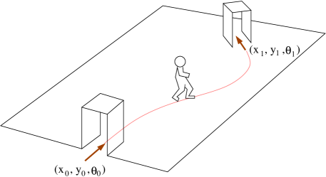
Figure 1: Goal-oriented human locomotion.

A nowadays widely accepted paradigm in neurophysiology is that, among all possible movements, the accomplished ones satisfy suitable optimality criteria (see [15] for a review). One is then led to make the assumption that the chosen locomotor trajectory is solution of some optimal problem, namely: minimize some integral cost

$$\mathcal{C}=\int L(x,y,\theta,\dot{x},\dot{y},\dot{\theta},\dots)dt$$

among all “admissible” trajectories joining the initial point to the final one. Two questions are in order. First, what are the “admissible” trajectories? It is in particular necessary to precise both the dynamical constraints applied to the locomotion, and the regularity of the trajectories (and so the order of derivation entering in the cost function $L$). Secondly, how to choose the cost function? Once the set of admissible trajectories is defined, the latter question takes the form of an inverse optimal control problem: given recorded experimental data, infer a cost function $L$ such that the recorded trajectories are optimal solutions of the associated minimization problem.

In the theory of linear-quadratic control, the question of which quadratic cost is minimized in order to control a linear system along certain trajectories was already raised by R. Kalman [10]. Some methods allowed deducing cost functions from optimal behaviour in system and control theory (linear matrix inequalities, [7]) and in Markov decision processes (inverse reinforcement learning, [13]). However all these methods have been conceived for very specific systems and they are not suitable in the general case. A new and promising approach of the inverse optimal control problem has been developped in [6, 9] for the pointing movements of the arm. In that approach, based on Thom transversality theory, the cost structure is deduced from qualitative properties highlighted by the experimental data. Thus, starting from the observation of inactivity intervals of the muscles during pointing movements, it has been proven that their presence is a sort of necessary and sufficient condition for the cost to be of a certain type (namely of “absolute work” type).

The method chosen in the present paper bears some resemblance with  [6, 9]. However no strong qualitative properties such as the inactivations come out in the registered data, which prevent the use of transversality theory. We then choose a more direct approach, consisting of three steps:

1. Modeling step: use experimental observations to define the set of admissible trajectories and to reduce the class of acceptable cost functions $L$; as a result, we obtain a class of optimal control problems indexed by the cost function $L$.

2. Analysis step: make a qualitative analysis of the optimal synthesis of the above-defined problems; the aim is mainly to exhibit properties characterizing the dependence on $L$ of the synthesis.

3. Comparison step: through a numerical study based on the characteristic properties exhibited above and a comparison with the trajectories experimentally recorded, determine which is the cost function $L$ which best fits the experimental data.

The last step is of different nature than the first two ones. It requires the processing of a large number of registered data together with a numerical study. In this paper we will then be concerned only with the first two steps, the last one being the object of a forthcoming study. Note that in the paper [5] we already performed a similar analysis for a simplified model.

The modeling step will be addressed in Section 2 and comes up with an optimal control problem (OCP). It is based on experimental observations together with two modeling assumptions, (A1) and (A2), and also on technical hypothesis, (H1)–(H4).

Section 3 is dedicated to the analysis step, all the technical proofs being postponed to Section 4. We first show the existence of optimal solutions and apply the Pontryagin maximum principle to Problem (OCP). After a detailed analysis of the extremal flow, we show that the angle $\theta$ along an optimal trajectory is solution of a fourth-order differential equation $(OPT)_{p}$ with parameter $p$. In case the initial point and the target are far enough one from each other, we are able to compute the asymptotic value $p^{*}$ of the parameter and to prove that the orbit corresponding to an optimal trajectory lies in the stable manifold of the (unique) unstable equilibrium of $(OPT)_{p^{*}}$. This asymptotic behavior exactly provides the type of characteristic properties of the trajectories of human locomotion we are looking for in order to test the adequacy of the model to registered data. The latter task will be the subject of a future work.

Moreover, based on the above asymptotic property, one can device a numerical method for determining the initial value of the adjoint vector and thus completely integrating the extremal flow. From the point of view of optimal control, this geometric method is the main technical novelty of our paper. It belongs to the realm of indirect methods, but is clearly of different nature than the shooting methods.

2 Optimal control based modeling

The first task is to define what is the set of admissible trajectories. It is important here to precise the typical situation we want to model, namely a person entering a room through one door and leaving by another one. Hence, besides the fact that initial and final positions and orientations are fixed, the velocity is positive at the extremities (the person walks in and out the room). Moreover the two doors, and so initial and final positions, are supposed not too close one to the other.

Our modeling is based on three important experimental observations made in [2, 3].

Figure 2: The nonholonomic constraint.

1. The velocity is perpendicular to the body (see Figure 2). Namely, denoting by $\theta$ the orientation of the torso and by $(x,y)$ the horizontal projection of the center of mass, the locomotion is submitted to the classical nonholonomic constraint:

   $$\dot{x}\sin\theta-\dot{y}\cos\theta=0,\qquad\hbox{i.e.}\quad\left\{\begin{array}[c]{l}\dot{x}=v\cos\theta\\ \dot{y}=v\sin\theta\end{array}\right.$$

   where $v=\sqrt{\dot{x}^{2}+\dot{y}^{2}}$ is the tangential velocity.

2. The tangential velocity has a positive lower bound: $v\geq a>0$. As a consequence, all locomotion trajectories can be parametrized by the arc-length. We are interested here in the geometric curves of the human locomotion, not by their time-parametrized trajectories. We will then use the arc-length parametrization, which amounts to set $v\equiv 1$.

   It is worth to notice that, on recorded data, the tangential velocity is generally almost constant along the trajectory. Thus, up to rescaling, arc-length and time parametrization approximately coincide.

3. The curvature varies continuously. That is, $\kappa(t)=\dot{\theta}(t)$ is a continuous function.

It results from these observations that every locomotion trajectory satisfies

$$\dot{x}=\cos\theta,\quad\dot{y}=\sin\theta,\quad\dot{\theta}=\kappa,$$

where $\kappa$ is a continuous function. Thus $\dot{x},\dot{y}$ and all their derivatives only depends on $\theta$ and its derivatives. To complete the description of the set of admissible trajectories, it only remains to precise in which functional space is chosen the function $\theta$. Remind that our main modeling assumption is that human locomotion is governed by optimality criteria. It is then mandatory to choose a functional space for the trajectories together with a class of cost functions so that one has general results ensuring the existence of optimal solution under reasonable hypothesis. As for the functional space, it must be complete and the natural choice is that of the Sobolev spaces $W^{k,p}$. In other words, we assume that the locomotion trajectories are solutions of the control system

$$\begin{cases}\dot{x}=\cos\theta,\\ \dot{y}=\sin\theta,\\ \theta^{(k)}=u,\end{cases}$$

where $u$ is a measurable function of finite $L^{p}$ norm, for a certain integer $p>0$, and $k>0$ is an integer. As for the cost functions $L$, the highest order of derivatives of $\theta$ actually appearing in $L$ must be equal to $k$. The observation $(iii)$ above suggests that the order $k$ is at least equal to two. We will make here the assumption that it is exactly equal to two.

• The cost function $L=L(x,y,\theta,\dot{\theta},\ddot{\theta})$ explicitly depends on $\ddot{\theta}$, and the latter has a finite $L^{p}$ norm.

To sum up, the control system modeling the dynamics of the locomotion writes as:

$${}\begin{cases}\dot{x}=\cos\theta,\\ \dot{y}=\sin\theta,\\ \dot{\theta}=\kappa,\\ \dot{\kappa}=u,\end{cases}$$ (2.1)

where $X=(x,y,\theta,\kappa)$ belongs to ${\mathbb{R}}^{2}\times S^{1}\times{\mathbb{R}}$ and the control $u$ is a measurable function defined on an interval $[0,T]$, where $T>0$ depends on $u$, and taking values in ${\mathbb{R}}$.

As for the initial and final points $X_{0},X_{1}$, the spatial and angular components $(x,y,\theta)$ are given by the data of the goal-oriented locomotion problem we consider. Two reasonable conditions could be assumed on the curvature:

• either $\kappa$ is let free, the cost $\mathcal{C}(u(\cdot))$ being minimized among all the points $X_{0},X_{1}$ with fixed spatial and angular components;

• or it satisfies $\kappa=0$ at $X_{0},X_{1}$ (the trajectory starts and ends in straight line).

This second hypothesis corresponds to the particular experimental setting considered in [2]. In this paper we will follow this assumption, however the other one essentially leads to the same results and we will mention in Section 3.5 how they differ.

The locomotion trajectories between two arbitrary configurations $(x_{0},y_{0},\theta_{0})$ and $(x_{1},y_{1},\theta_{1})$ then appear as the solutions of an optimal control problem of the following form: minimize the cost

$$\mathcal{C}(u(\cdot))=\int_{0}^{T}L(x,y,\theta,\kappa,u)dt$$

among all admissible controls $u(\cdot)$ steering System 2.1 from $X(0)=(x_{0},y_{0},\theta_{0},0)$ to $X(T)=(x_{1},y_{1},\theta_{1},0)$. Notice that the time is free in this problem, $T$ depends on $u(\cdot)$.

The inverse optimal control problem consists in finding the proper cost function $L$. Some elementary remarks allows us to reduce the class of the candidates.

1. The cost function is defined in an egocentric frame; the whole problem is then invariant by rototranslations, and $L$ is independent of $(x,y,\theta)$, that is,

   $$L=L(\kappa,u).$$

2. Turning right or left are equivalent, hence the symmetry of $L$ : $L(-\kappa,-u)=L(\kappa,u)$.

3. The more one turns, the more it costs. In other words, the partial functions $\kappa\mapsto L(\kappa,u)$ and $u\mapsto L(\kappa,u)$ are non-decreasing function of $|\kappa|$ and $|u|$ respectively.

4. Going in straight line has a positive cost, $L(0,0)>0$, which is the unique minimum of $L$. Since $L$ is defined up to a multiplicative constant, we can impose the normalization: $L(0,0)=1$ and $L(\kappa,u)>1$ for $(\kappa,u)\neq 0$. As a consequence, the cost of a straight line is its Euclidean length.

5. As already mentioned, the optimal control problem must have a solution, which requires some convexity properties on $L$.

In this paper, we will restrict the class of cost functions satisfying the following assumption:

• The cost function $L$ depends separately on $\kappa$ and $u$.

We will then consider a cost

$$\mathcal{C}(u(\cdot))=\int_{0}^{T}[1+\varphi(\kappa(t))+\psi(u(t))]dt.$$ (2.2)

This cost appears as a compromise between the total time $T$ (equivalently, the length to be covered) and an “energy term” depending separately on $\kappa$ and $u$.

To satisfy the properties listed above we assume that the functions $\varphi$ and $\psi$ verify the following technical hypotheses.

• $\varphi$ and $\psi$ are non negative, $\mathcal{C}^{2}$ and even functions defined on ${\mathbb{R}}$, and are non decreasing on ${\mathbb{R}}^{+}$. Moreover, $\varphi(0)=\psi(0)=0$;

• $\psi$ is strictly convex and $\psi^{\prime\prime}(0)>0$;

• there exist $p>1$ and two positive constants $C,R$ such that

  $$\psi(r)\geq C|r|^{p},\hbox{ for every }r\in{\mathbb{R}}\hbox{ such that }|r|\geq R.$$ (2.3)

We next provide some explanations about these hypotheses.

Hypothesis (H1) directly results from properties $(ii)$–$(iv)$ and is structural to the model, except for the regularity assumption. However, if the cost was not differentiable, the phenomenon of “inactivation” would appear in the optimal trajectories (see [9]). Since inactivation is not observed in the registered data, one must assume some regularity property for the cost. Note that the $\mathcal{C}^{2}$ regularity of $\varphi$ and $\psi$ required in (H1) is actually needed just for the development of the numerical method of Section 3.4, while the qualitative results of Sections 3.2 and 3.3 are valid even if we assume that $\varphi$ and $\psi$ are just $\mathcal{C}^{1}$.

The convexity and the growth condition provided by Hypotheses (H2)–(H3) are classical assumptions which ensure Property $(v)$ (see Proposition 3.1 and Remark 3.2 below). The technical assumption $\psi^{\prime\prime}(0)>0$ ensures that, firstly the minimizers are locally unique; secondly they are solutions of an ODE (of pendulum-type); and thirdly one can recover at least numerically the initial value of the adjoint vector (in an approach based on the Pontryagin maximum principle). It is worth to notice that (H2)–(H3) define open conditions on the set of functions $\varphi$ and $\psi$ satisfying (H1). This stability property is necessary due to the physiological nature of the cost.

The purpose of Assumption (A2) is to ensure that Property $(v)$ is satisfied with reasonable hypotheses like (H2)–(H3) (see, for instance, [12] for a discussion about existence of minimizers under similar assumptions).

To summarize, the optimal control problem modeling the goal-oriented human locomotion is the following one.

(OCP) Fix an initial point $X_{0}=(0,0,\pi/2,0)$. For every final point of the form $X_{1}=(x_{1},y_{1},\theta_{1},0)$, for some $(x_{1},y_{1},\theta_{1})\in{\mathbb{R}}^{2}\times S^{1}$, find the trajectories of (2.1) steering the system from $X_{0}$ to $X_{1}$ and minimizing the cost (2.2), where $\varphi$ and $\psi$ verify hypothesis (H1)–(H4).

3 Qualitative analysis of the optimal trajectories

3.1 Notations

In the following we will make use of the following notations.

We will always assume without loss of generality that the difference $\alpha_{1}-\alpha_{2}$ between two angles $\alpha_{1},\alpha_{2}\in[0,2\pi]$ takes values in the interval $[-\pi,\pi]$. In particular with this notation the modulus $|\alpha_{1}-\alpha_{2}|$ is a continuous function of $\alpha_{1},\alpha_{2}$ taking values in $[0,\pi]$.

Given a subset $S$ of $[0,T]$ we will denote its complement in $[0,T]$ by $S^{c}$.

The Lebesgue measure of a set $S$ will be denoted by $\mu(S)$.

The scalar product in ${\mathbb{R}}^{2}$ is denoted by $\left\langle\cdot,\cdot\right\rangle$.

The symbol $B(x,r)$ indicates the ball of radius $r$ centered at $x$.

As usual, given two subsets $A,B$ of a certain vector space the set $A+B$ is defined as

$$A+B=\{x+y\,:\,x\in A,\,y\in B\}.$$

3.2 Existence of optimal trajectories

The existence of solutions to problem (OCP) is guaranteed by the following result.

Proposition 3.1.

For every choice of $X_{0}$ and $X_{1}$ in ${\mathbb{R}}^{2}\times\mathcal{S}^{1}\times{\mathbb{R}}$ there exists a trajectory $\bar{X}(\cdot)$ of (2.1), defined on $[0,\bar{T}]$, associated to some control $\bar{u}(\cdot)$ and minimizing $\mathcal{C}(u(\cdot))$ among all the trajectories starting from $X_{0}$ and reaching $X_{1}$.

Proof. Consider a minimizing sequence $u_{n}(\cdot):[0,T_{n}]\rightarrow{\mathbb{R}}$, that is

$$\lim_{n\to\infty}\mathcal{C}(u_{n}(\cdot))=\inf_{u(\cdot)}\mathcal{C}(u(\cdot))$$

where $u_{n}(\cdot),u(\cdot)$ steer the system from $X_{0}$ to $X_{1}$. Since $\mathcal{C}(u_{n}(\cdot))$ is uniformly bounded, one easily deduces from Hypothesis (H1) and (H3) that $T_{n}$ and $\|u_{n}\|_{L^{p}([0,T_{n}])}$ must be uniformly bounded, and therefore, up to a subsequence, we can assume that $T_{n}$ converges to $\bar{T}$. Let us extend $u_{n}(\cdot)$ on $[0,\infty)$ by taking $u_{n}(t)=0$ if $t>T_{n}$. Then, still up to subsequences, $u_{n}(\cdot)$ converges to some $\bar{u}(\cdot)\in L^{p}([0,\bar{T}])$ in the weak topology of $L^{p}([0,\bar{T}])$. Moreover, the functions $\kappa_{n}(t)=\int_{0}^{t}u_{n}(s)ds$ are uniformly continuous by Hölder’s inequality and they converge pointwise to $\bar{\kappa}(t)=\int_{0}^{t}\bar{u}(s)ds$ since $u_{n}(\cdot)\rightharpoonup\bar{u}(\cdot)$ in $L^{p}$. By Ascoli-Arzelà theorem, $\kappa_{n}$ converge to $\bar{\kappa}$ uniformly on $[0,\bar{T}]$. Therefore, from the equation (2.1), we immediately get that the trajectories $X_{n}(\cdot)$ corresponding to $u_{n}(\cdot)$ converge uniformly to the trajectory $\bar{X}(\cdot)$ corresponding to $\bar{u}(\cdot)$ and, since these trajectories are uniformly equi-continuous, $\bar{X}(\bar{T})=\lim_{n\to\infty}X_{n}(T_{n})=X_{1}$. Moreover, we deduce that the sequence $\Big{(}\int_{0}^{T_{n}}\varphi(\kappa_{n}(t))dt\Big{)}_{n}$ converges to $\int_{0}^{\bar{T}}\varphi(\bar{\kappa}(t))dt$.

Let us denote $L_{0}(u(\cdot),T)=\int_{0}^{T}\psi(u(t))dt$. It remains to prove that $L_{0}(\bar{u}(\cdot),\bar{T})=\lim_{n\to\infty}L_{0}(u_{n}(\cdot),T_{n})$. For this purpose, we first observe that the convexity of $\psi(\cdot)$ immediately implies the convexity in $L^{p}([0,\bar{T}])$ of the functional $L_{0}(\cdot,\bar{T})$. It is well-known that the weak lower semi-continuity of a convex functional is equivalent to its strong lower semi-continuity (see for instance [8, Corollaire III.8]). From this fact, and since $L_{0}(u_{n}(\cdot),\bar{T})\leq L_{0}(u_{n}(\cdot),T_{n})$, to conclude the proof of the proposition it is enough to show that $L_{0}(\cdot,\bar{T})$ is strongly lower semi-continuous in $L^{p}([0,\bar{T}])$. Let us consider a sequence $(v_{k})_{k\geq 1}$ in $L^{p}([0,\bar{T}])$ converging in the $L^{p}$ norm to a function $v$. In particular we can extract a subsequence $(v_{k_{j}})_{j\geq 1}$ converging almost everywhere to $v$ and such that $\lim_{j\to\infty}L_{0}(v_{k_{j}}(\cdot),\bar{T})=\liminf_{k\to\infty}L_{0}(v_{k}(\cdot),\bar{T})$. According to Egoroff theorem there exists a sequence $(A_{h})_{h\geq 1}$ of open nested subsets of $[0,\bar{T}]$ such that $\lim_{h\to\infty}\mu(A_{h})=0$ and the convergence $v_{k_{j}}\to v$ is uniform in $[0,\bar{T}]\setminus A_{h}$. We get

$$L_{0}(v(\cdot),\bar{T}) = \lim_{h\to\infty}\left(L_{0}(v(\cdot),\bar{T})-\int_{A_{h}}\psi(v(\tau))d\tau\right)$$

$$= \lim_{h\to\infty}\lim_{j\to\infty}\left(L_{0}(v_{k_{j}}(\cdot),\bar{T})-\int_{A_{h}}\psi(v_{k_{j}}(\tau))d\tau\right)$$

$$\leq \lim_{j\to\infty}L_{0}(v_{k_{j}}(\cdot),\bar{T})$$

which concludes the proof of the proposition. $\Box$

Remark 3.2.

The argument we provided is inspired from the proof of Theorem 8, p. 209 of [12]. Let us stress that it is not difficult to show through appropriate examples that the convexity of $\psi$ required by Hypothesis (H2) is crucial for the existence of a minimizer.

3.3 Application of the Pontryagin maximum principle

In order to apply the classical Pontryagin maximum principle (PMP) [14], one needs to know that the optimal control $\bar{u}(\cdot)$ is bounded in the $L^{\infty}$ topology. At the present stage of the analysis, we do not possess that information and we therefore must rely on more sophisticated versions of the PMP. For instance, one readily checks that (OCP) meets all the hypotheses required in Theorem 2.3 of [4] and we get the following.

Proposition 3.3.

Let $\bar{X}(\cdot)$ be an optimal trajectory for (OCP), defined on $[0,\bar{T}]$ and associated to the control $\bar{u}(\cdot)$. Then this trajectory satisfies the PMP.

Let us associate to System (2.1) the Hamiltonian function

$${}H=H(X,p,u,\nu)=p_{1}\cos\theta+p_{2}\sin\theta+p_{3}\kappa+p_{4}u-\nu(1+\varphi(\kappa)+\psi(u)),$$ (3.1)

where $p=(p_{1},p_{2},p_{3},p_{4})\in\mathbb{R}^{4}$ is the adjoint vector and $\nu\in{\mathbb{R}}$.

The PMP writes as follows. Let $u(\cdot)$ be an optimal control defined on the interval $[0,T]$ and $X(\cdot)$ the corresponding optimal trajectory, whose existence is guaranteed by Proposition 3.1. Then $X(\cdot)$ is an extremal trajectory, i.e. it satisfies the following conditions. There exists an absolutely continuous function $p:[0,T]\rightarrow\mathbb{R}^{4}$ and $\nu\geq 0$ such that the pair $(p(\cdot),\nu)$ is non-trivial, and such that we have:

$${}\begin{cases}\dot{X}(t)=\frac{\partial H}{\partial p}(X(t),p(t),\nu,u(t)),\\ \dot{p}(t)=-\frac{\partial H}{\partial X}(X(t),p(t),\nu,u(t)).\end{cases}$$ (3.2)

The maximization condition writes:

$${}H(X(t),p(t),u(t),\nu)=\max_{v\in{\mathbb{R}}}H(X(t),p(t),v,\nu)\ \mathrm{for}\ a.e.\ t\in[0,T].$$ (3.3)

As the final time is free, the Hamiltonian is zero (see [16]):

$${}H(X(t),p(t),u(t),\nu)=0,\hskip 5.69046pt\forall t\in[0,T].$$ (3.4)

The equation on the covector $p$, also called adjoint equation, becomes:

$${}\begin{cases}\dot{p}_{1}=0,\\ \dot{p}_{2}=0,\\ \dot{p}_{3}=p_{1}\sin\theta-p_{2}\cos\theta,\\ \dot{p}_{4}=-p_{3}+\nu\varphi^{\prime}(\kappa).\end{cases}$$ (3.5)

If $\nu\neq 0$ we can always suppose, by linearity of the adjoint equation, that $\nu=1$. In this case (resp., if $\nu=0$) a solution of the PMP is called a normal extremal (resp., an abnormal extremal). It is easy to see that all optimal trajectories are normal extremals. Indeed, if $\nu=0$, then $p_{4}\equiv 0$ by the maximization condition (3.3). From $\dot{p}_{4}=0$, we immediately deduce that $p_{3}\equiv 0$ and, from $\dot{p}_{3}=0$, it remains $p_{1}\sin\theta-p_{2}\cos\theta\equiv 0$. From $H=0$, one also has $p_{1}\cos\theta+p_{2}\sin\theta\equiv 0$ and thus $p_{1}=p_{2}=0$. That contradicts the non-triviality of $(p,\nu)$.

Consequently, Equation (3.4) becomes

$$p_{1}\cos\theta+p_{2}\sin\theta+p_{3}\kappa+p_{4}u-(1+\varphi(\kappa)+\psi(u))=0.$$ (3.6)

As regards the maximization condition (3.3), the optimal control is given by

$$u_{opt}(t)=(\psi^{\prime})^{-1}(p_{4}(t))\quad\mathrm{for}\ t\in[0,T].$$ (3.7)

Note that the strict convexity and the growth condition on $\psi$ imply that $\psi^{\prime}$ realizes a bijection from ${\mathbb{R}}$ to ${\mathbb{R}}$ and thus its inverse is a continuous and strictly increasing function from ${\mathbb{R}}$ to ${\mathbb{R}}$.

From (3.5), we get that $p_{1}$ and $p_{2}$ are constant. Let us write $(p_{1},p_{2})=\rho(\cos\phi,\sin\phi)$ for some $\phi\in[0,2\pi)$ and $\rho>0$. Therefore from the Hamiltonian system (3.2) we get that, along an optimal trajectory, the following equation, independent of $u$, is satisfied for a.e. $t\in[0,T]$ and for a suitable choice of $(\rho,\phi)\in{\mathbb{R}}\times[0,2\pi)$,

$$\begin{cases}\dot{\theta}=\kappa,\\ \dot{\kappa}=(\psi^{\prime})^{-1}(p_{4}),\\ \dot{p}_{3}=\rho\sin(\theta-\phi),\\ \dot{p}_{4}=-p_{3}+\varphi^{\prime}(\kappa)\,.\end{cases}$$ (3.8)

Note that this equation implies that the function $\theta$ is solution of a fourth order differential equation of pendulum type depending on the parameters $(\rho,\phi)$.

Setting $(x_{1},y_{1})=|(x_{1},y_{1})|(\cos\alpha,\sin\alpha)$ for some $\alpha\in[0,2\pi)$, a careful analysis of this equation yields the following results.

Proposition 3.4.

There exists $R>0$ and $C>0$ such that, for every optimal trajectory with $|(x_{1},y_{1})|\geq R$ one has

$$\|(\kappa,p_{3},p_{4})\|_{L^{\infty}}\leq C\qquad\hbox{and}\qquad\|u\|_{L^{\infty}}\leq C.$$

Remark 3.5.

The boundedness on $\|\kappa\|_{L^{\infty}}$ is valid without any hypothesis on $|(x_{1},y_{1})|$.

Proposition 3.6.

For every $\eta>0$ there exists $R_{\eta}>0$ such that for every optimal trajectory with $|(x_{1},y_{1})|\geq R_{\eta}$ one has

$$|\phi-\alpha|\leq\eta\qquad\hbox{and}\qquad|\rho-1|\leq\eta$$

Theorem 3.7.

Let us associate to any extremal trajectory $X(\cdot)$ of (OCP) the function $Z(t)=(\theta(t),\kappa(t),p_{3}(t),p_{4}(t))$. Given $\nu>0$ there exist $\tau_{\nu}>0$ and $\sigma_{\nu}>2\tau_{\nu}$ such that, for every optimal trajectory with final time $T>\sigma_{\nu}$, one has

$$|Z(t)-(\alpha,0,0,0)|<\nu\qquad\hbox{for }t\in[\tau_{\nu},T-\tau_{\nu}].$$

The proof of these results is rather long and technical, it is postponed to Section 4.3 for Propositions 3.4 and 3.6, and Section 4.4 for Theorem 3.7.

3.4 Numerical study of the asymptotic behavior

The main information provided in the previous section concerning optimal trajectories, solutions of (OCP), can be summarized as follows:

• if the norm of the spatial components $(x_{1},y_{1})$ of $X_{1}$ is large enough then optimal trajectories can be decomposed in three pieces corresponding to time intervals $[0,\bar{t}]$, $[\bar{t},T-\bar{t}]$, $[T-\bar{t},T]$, where $\bar{t}$ can be thought independent of $X_{1}$ and the arc of the trajectory on $[\bar{t},T-\bar{t}]$ is approximately a segment (the accuracy of the approximation depends on the size of $\bar{t}$);

• for any optimal trajectory there exist two scalars $(\rho,\phi)$ such that $Z(\cdot)=(\theta(\cdot),\kappa(\cdot),p_{3}(\cdot),p_{4}(\cdot))$ satisfies Equation (3.8). Also, the relation

  $$\hat{H}(\theta,\kappa,p_{3},p_{4}):=\rho\cos(\theta-\phi)+p_{3}\kappa+p_{4}(\psi^{\prime})^{-1}(p_{4})-1-\varphi(\kappa)-\psi\big{(}(\psi^{\prime})^{-1}(p_{4})\big{)}=0$$ (3.9)

  holds along the trajectory. Moreover, if $(x_{1},y_{1})$ is large enough, $\rho$ is close to $1$ and $\phi$ is close to the angle $\alpha$ such that $(x_{1},y_{1})=|(x_{1},y_{1})|(\cos\alpha,\sin\alpha)$.

The qualitative properties stressed above do not allow neither to understand the local behavior of optimal trajectories, in particular on the intervals $[0,\bar{t}],\,[T-\bar{t},T]$ defined by the above Condition (1), nor to find them numerically. However they detect some non-trivial asymptotic behavior of the pair $(\rho,\phi)$ and of the initial data of (3.8), for large values of $(x_{1},y_{1})$. The analysis carried out in this section arises from the observation that, in order to understand the asymptotic shape of the optimal trajectories on $[0,\bar{t}],\,[T-\bar{t},T]$, it would be enough to complete the information about the initial data of (3.8). Indeed, as far as the initial datum of the equation is close to its asymptotic value (if it exists) and $(\rho,\phi)$ is close to $(1,\alpha)$, we know, from classical continuous dependence results for the solutions of differential equations, that the solution of (3.8). will in turn be close (on compact time intervals) to the solution of the asymptotic equation

$$\left\{\begin{array}[]{l}\dot{\theta}=\kappa,\\ \dot{\kappa}=(\psi^{\prime})^{-1}(p_{4}),\\ \dot{p}_{3}=\sin(\theta-\alpha),\\ \dot{p}_{4}=-p_{3}+\varphi^{\prime}(\kappa).\end{array}\right.$$ (3.10)

where we take as initial value the asymptotic value of the initial data for (3.8). In other words, a precise knowledge of the asymptotic behavior of such initial data, for large $(x_{1},y_{1})$, would provide a tool to study numerically, through (3.10), the asymptotic shape of optimal trajectories on $[0,\bar{t}]$ (and, by symmetry, on $[T-\bar{t},T]$).

Let us first notice that an asymptotic value for $p_{4}(0)$ is simply provided by evaluating (3.9) at time $0$, with the approximation $(\rho,\phi)=(1,\alpha)$. More precisely $p_{4}(0)$ coincides with a solution $z$ of the equation

$$\cos(\pi/2-\alpha)+z\,(\psi^{\prime})^{-1}(z)-1-\psi\big{(}(\psi^{\prime})^{-1}(z)\big{)}=0\,.$$ (3.11)

Since the map $\eta\mapsto\psi^{\prime}(\eta)\eta-\psi(\eta)=\int_{0}^{\eta}(\psi^{\prime}(\eta)-\psi^{\prime}(\mu))\,d\mu$ is strictly increasing for $\eta\geq 0$, strictly decreasing for negative $\eta$ and goes to infinity for $|\eta|$ going to infinity, because of the strict convexity of $\psi$, and since $\psi\in\mathcal{C}^{1}$, we know that the previous equation has exactly one positive solution and one negative solution. Since $u(0)=(\psi^{\prime})^{-1}(p_{4}(0))$, this suggests the existence of two asymptotic behaviors for the trajectories of (3.8), each one corresponding to a candidate solution for (OCP). These two trajectories start from $X_{0}$ by turning on opposite directions.

To complete the information about the asymptotic value of the initial data for (3.8) we need to investigate the possible values of $p_{3}(0)$. For this purpose we will develop below a numerical method based on the existence of a stable manifold for (3.10).

An equilibrium for (3.10) is given by $(\theta,\kappa,p_{3},p_{4})=(\alpha,0,0,0)$ and we know from Theorem 3.7 that, for solutions of (OCP) with $(x_{1},y_{1})$ far enough from the origin, the corresponding values of $(\theta(\cdot),\kappa(\cdot),p_{3}(\cdot),p_{4}(\cdot))$ are close to this equilibrium on some interval $[\bar{t},T-\bar{t}]$ for large $\bar{t}$ and $T$, which suggests some stability property of the equilibrium. It is actually easy to see that $Z_{eq}=(\alpha,0,0,0)$ is not a stable equilibrium of the system. Indeed the linearized system around $Z_{eq}$ is

$$\dot{Z}=J(Z-Z_{eq})\,,\quad J=\left(\begin{array}[]{cccc}0&1&0&0\\ 0&0&0&1/\psi^{\prime\prime}(0)\\ 1&0&0&0\\ 0&\varphi^{\prime\prime}(0)&-1&0\end{array}\right)\,,\quad Z\in{\mathbb{R}}^{4},$$ (3.12)

where the matrix $J$ has exactly two eigenvalues $\lambda_{1},\lambda_{2}$ with negative real part, corresponding to some eigenvectors $v_{1},v_{2}$, while the other two eigenvalues $\mu_{1},\mu_{2}$, with corresponding eigenvectors $w_{1},w_{2}$, have positive real part. Therefore $Z_{eq}$ is a stable equilibrium for the linearized dynamics restricted to $Z_{eq}+V$, where $V$ is the two dimensional real subspace of ${\mathbb{R}}^{4}$ spanned by $v_{1},v_{2}$ (notice that $v_{1},v_{2}$ can be assumed either real or complex conjugate).

The classical stable manifold theorem (see for instance [11]) ensures the existence of a manifold $\mathcal{W}^{s}$ of dimension $2$, called stable manifold, which is tangent to $V$ and which contains all the trajectories converging to the equilibrium (exponentially fast). Note that, since the continuous function $\hat{H}$, with $(\rho,\phi)=(1,\alpha)$, is a first integral of the dynamics (3.10) and $\hat{H}(Z_{eq})=0$ we have $\mathcal{W}^{s}\subset\hat{H}^{-1}(0)$.

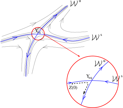
Figure 3: Behavior around the stable and unstable manifolds.

On a small neighborhood of the equilibrium all the trajectories that are not contained in $\mathcal{W}^{s}$ diverge from it exponentially fast (see Figure 3). Let us fix such a neighborhood $U$. From Theorem 3.7 we know that there exists $\bar{t}$ such that, if $Z(\cdot)$ is a trajectory of (3.8) associated to a solution of (OCP), then $Z(t)\in U$ for every $t\in[\bar{t},T-\bar{t}]$, provided that $(x_{1},y_{1})$ is far enough from the origin. In particular if we consider a sequence of final points $X_{1}^{(n)}$ for (OCP) with spatial components $(x_{1}^{(n)},y_{1}^{(n)})=n(\cos\alpha,\sin\alpha)$ we deduce that, for the corresponding sequence of trajectories $Z^{(n)}(\cdot)$, the limit $\bar{Z}$ of $Z^{(n)}(\bar{t})$ exists (up to a subsequence) and is contained in $\mathcal{W}^{s}$. Continuous dependence results for the solutions of differential equations guarantee that the limit of $Z^{(n)}(0)$ coincides with $\bar{Z}(0)$, where $\bar{Z}(\cdot)$ is the solution of (3.10) such that $\bar{Z}(\bar{t})=\bar{Z}$. In particular it must be $\bar{Z}(0)=(\pi/2,0,\bar{p}_{3},\bar{p}_{4})$ where $\bar{p}_{4}$ satisfies (3.11).

The previous reasoning suggests a method to study numerically the possible values of $\bar{p}_{3}$ at time $0$. Indeed if $U$ is small enough then $\mathcal{W}^{s}$ is well approximated by the affine space $Z_{eq}+V$. Consequently one can numerically look for solutions of the asymptotic equation (3.10) with

$$Z(\bar{t})\in(Z_{eq}+V)\cap U$$

and such that $\theta(0)=\pi/2,\,\kappa(0)=0$. More precisely a simple numerical method can be specified as follows. Let us fix a closed curve $\gamma(s)=\varepsilon\,(\cos(s)\bar{v}_{1}+\sin(s)\bar{v}_{2})$, where $\bar{v}_{1},\bar{v}_{2}$ are real vectors spanning $V$ and $\varepsilon$ is a small constant (the precision of the method increases as $\varepsilon$ goes to zero). Since all the trajectories converging to the equilibrium must cross this curve (in the approximation $\mathcal{W}^{s}\simeq Z_{eq}+V$) we can recover them by following backwards in time the solutions of (3.10) starting at $Z(0)=Z_{eq}+\gamma(s)$ up to a time $\tilde{t}<0$ such that $\kappa(\tilde{t})=0$. The candidate approximate asymptotic trajectories we are looking for are then determined by the values of $s$ for which, for a reasonably not too large $|\tilde{t}|$ such that $\kappa(\tilde{t})=0$, we also have $\theta(\tilde{t})=\pi/2$. The value $Z(0)$ is then a candidate value for the initial datum of a trajectory of (3.8) associated to a solution of (OCP), for large values of $(x_{1},y_{1})$. Moreover this simple method allows to approximate numerically the initial arc of such optimal trajectories (see Figure 4 which considers the case $\varphi\equiv 0,\,\psi(z)=z^{2}$).

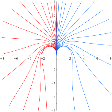
Figure 4: Asymptotic behavior of optimal trajectories with final point far from the origin.

An effective method to globally construct solutions of (OCP) for large values of $(x_{1},y_{1})$ is the following. Define a further closed curve $\hat{\gamma}(\hat{s})=\hat{\varepsilon}\,(\cos(\hat{s})\bar{w}_{1}+\sin(\hat{s})\bar{w}_{2})$, where $\bar{w}_{1},\,\bar{w}_{2}$ are real vectors generating the unstable subspace $W$ (defined similarly to $V$). Assume that $\hat{\varepsilon}\ll\varepsilon\ll 1$ and consider the solutions of (3.8) with $\phi=0$ and starting from $Z(0)=\gamma(s)+\hat{\gamma}(\hat{s})$, for suitable choices of $\rho,\varepsilon,\hat{\varepsilon},s,\hat{s}$ such that $\hat{H}(Z(0))=0$. For a fixed small enough $\varepsilon>0$ and fixed $s\in[0,2\pi]$ it turns out that the trajectory on intervals $[t_{1},0]$, with $t_{1}<0$ not too large, is subjected to small variations with respect to the choice of $\hat{\varepsilon}\ll\varepsilon,\hat{s}\in[0,2\pi],\rho$ such that $\hat{H}(Z(0))=0$. In other words the trajectory approximately only depends on $\varepsilon,s$ on the interval $[t_{1},0]$. Similarly as before, the value $s$ and the time $t_{1}$ can be chosen in such a way that $\kappa(t_{1})=0$ and, at the same time, $\theta(t_{1})=\pi/2-\phi$, for a prescribed value $\phi$.

On the other hand for positive time the components along the stable subspace $V$ decrease exponentially as far as the components along $W$ are small so that, after a certain time, the trajectory evolves close to the unstable manifold $\mathcal{W}^{u}$ (see Figure 3). The dynamics at this stage essentially depends on the initial choice of $\hat{\varepsilon}$ and $\hat{s}$, where the first parameter determines the range of time such that the trajectory is confined inside $U$, while the second one essentially determines the final angle.

This method gives rise, up to a rotation of an angle $\phi$ and appropriate translations, to solutions of (OCP). Figure 5 depicts a set of candidate solutions of (OCP) constructed by using the previous method, for a particular choice of the angle $\phi$ and in the case $\varphi\equiv 0,\psi(z)=z^{2}$.

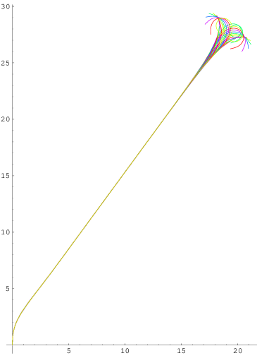
Figure 5: Candidate optimal trajectories for large values of $(x_{1},y_{1})$.

3.5 The case with free curvature at the extremities

In the definition of the optimal control problem (OCP) given in Section 2, we have chosen to take the initial and final values of the curvature equal to 0. Another reasonable condition would be to let these values free. In this case, the optimal control problem writes as follows.

$(\mathbf{\widetilde{OCP}})$ Fix an initial point $Q_{0}=(0,0,\pi/2)$ in coordinates $(x,y,\theta)$. For every final point $Q_{1}=(x_{1},y_{1},\theta_{1})\in{\mathbb{R}}^{2}\times S^{1}$, find the trajectories $X(\cdot)=(x(\cdot),y(\cdot),\theta(\cdot),\kappa(\cdot))$ of (2.1) such that $(x(0),y(0),\theta(0))=Q_{0}$ and $(x(T),y(T),\theta(T))=Q_{1}$, and minimizing the cost (2.2) under hypotheses (H1)–(H4).

The analysis of $(\mathbf{\widetilde{OCP}})$ leads essentially to the same results than the one of (OCP). The only noticeable differences are the following ones.

• When applying the PMP, in addition to the Hamiltonian equations (3.2), one obtain also a transversality condition on $(p(0),p(T))$, namely

  $$p_{4}(0)=p_{4}(T)=0.$$

  These conditions play the same role than the condition $\kappa(0)=\kappa(T)=0$ in (OCP).

• In Section 3.4, the relation (3.9) on the Hamiltonian allows to characterize the asymptotic value $\kappa(0)$ (and not the one of $p_{4}(0)$ through Equation (3.11) as in (OCP)), in function of $p_{3}(0)$. Indeed, since $p_{4}(0)=0$, one has, for the asymptotic values:

  $$\cos(\pi/2-\alpha)+p_{3}(0)\kappa(0)-1-\varphi(\kappa(0))=0.$$

  The numerical methods presented in Section 3.4 have to be slightly modified in accordance with the changes above.

Note also that the proof of Lemma 4.8 has to be modified (see Remark 4.9).

4 Proofs of the main results

4.1 Comparison with reference trajectories

In order to obtain a first rough estimate of the optimal cost, we exhibit particular trajectories of (2.1) steering the system from $X_{0}$ to $X_{1}$.

Proposition 4.1.

Given $\sigma>0$, a pair $(\lambda_{0},\lambda_{1})\in{\mathbb{R}}_{+}^{3}$ and $T\geq 2\lambda_{0}+2\lambda_{1}$ we define the control function

$$u(t)=\left\{\begin{array}[]{rl}-\sigma{}{}&t\in[0,\lambda_{0}]\\ +\sigma{}{}&t\in(\lambda_{0},2\lambda_{0}]\\ 0{}{}&t\in(2\lambda_{0},T-2\lambda_{1}]\\ +\sigma{}{}&t\in(T-2\lambda_{1},T-\lambda_{1}]\\ -\sigma{}{}&t\in(T-\lambda_{1},T]\end{array}\right.\,.$$ (4.1)

Then, for every choice of $X_{1}=(x_{1},y_{1},\theta_{1},0)$ with $|(x_{1},y_{1})|\geq 8\sqrt{\pi/\sigma}$, there exists a pair $(\lambda_{0},\lambda_{1})\in[0,\sqrt{3\pi/\sigma}]\times[0,\sqrt{5\pi/\sigma}]$ and $T\geq 2\lambda_{0}+2\lambda_{1}$ such that the trajectory of (2.1) with $u(\cdot)$ given by (4.1) starting at $X_{0}$ reaches $X_{1}$ at time $T$.

Figure 6: The function $\kappa(\cdot)$ associated to the control function of Proposition 4.1

Proof. First, let us observe that $\kappa=0$ along the arc corresponding to $u=0$, which is therefore a segment, and $\kappa(0)=\kappa(T)=0$ (see Figure 6). Also, since $\ddot{\theta}=u$, one can easily check that $\theta(t)=\theta_{0}-\sigma\lambda_{0}^{2}$ between $2\lambda_{0}$ and $T-2\lambda_{1}$ and that $\theta(T)=\theta_{0}-\sigma\lambda_{0}^{2}+\sigma\lambda_{1}^{2}$. Therefore, since it must be $\theta=\theta_{1}$ at the final time, and up to assuming without loss of generality that $\theta_{1}-\theta_{0}\in[0,2\pi)$, we can assume that $\lambda_{1}$ is the following continuous function of $\lambda_{0}\in[0,\sqrt{3\pi/\sigma}]$:

$$\lambda_{1}=\lambda_{1}(\lambda_{0})=\sqrt{\frac{\theta_{1}-\theta_{0}}{\sigma}+\lambda_{0}^{2}}\,.$$

Let us denote by $\gamma_{0}(\cdot)$ the trajectory of (2.1) corresponding to $u(\cdot)$ starting at $X_{0}$ at time $0$ and by $\gamma_{1}(\cdot)$ the trajectory of (2.1) corresponding to $u(\cdot)$ based at $X_{1}$ at time $T$. Our aim is to prove that, for an appropriate choice of $(\lambda_{0},T)$, these trajectories coincide. For this purpose it is enough to prove that their projections on the plane coincide.

Let us consider the points $P_{0}$ and $P_{1}$ which are the projections on the plane of $\gamma_{0}(2\lambda_{0})$ and $\gamma_{1}(T-2\lambda_{1})$ (see Figure 7). Since for both $\gamma_{0}(\cdot)$ and $\gamma_{1}(\cdot)$ the angle $\theta(\cdot)$ is constantly equal to $\alpha(\lambda_{0}):=\theta_{0}-\sigma\lambda_{0}^{2}$ on the interval $[2\lambda_{0},T-2\lambda_{1}]$, we deduce that the two curves coincide, up to an appropriate choice of $T>0$, if and only if the angle $\beta(\lambda_{0})$ between the vector $P_{1}-P_{0}$ and the horizontal axis is equal to $\alpha(\lambda_{0})$ (up to a multiple of $2\pi$).

Let us observe that $\lambda_{0}+\lambda_{1}\leq\sqrt{3\pi/\sigma}+\sqrt{5\pi/\sigma}\leq 4\sqrt{\pi/\sigma}$. Since $|P_{0}|<2\lambda_{0}$ and $|P_{1}-(x_{1},y_{1})|<2\lambda_{1}$ when $\lambda_{0}\neq 0$ and $\lambda_{1}\neq 0$, if $|(x_{1},y_{1})|\geq 8\sqrt{\pi/\sigma}$ then

$$\begin{array}[]{rcl}\left\langle(x_{1},y_{1}),P_{1}-P_{0}\right\rangle&=&\left\langle(x_{1},y_{1}),P_{1}-(x_{1},y_{1})\right\rangle+\left\langle(x_{1},y_{1}),(x_{1},y_{1})\right\rangle-\left\langle(x_{1},y_{1}),P_{0}\right\rangle\\ &\geq&|(x_{1},y_{1})|^{2}-2(\lambda_{0}+\lambda_{1})|(x_{1},y_{1})|\\ &\geq&0\,.\end{array}$$

This implies that $\beta(\cdot)$ takes values on an interval of length less than $\pi$. Moreover, since $P_{0}$ and $P_{1}$ are continuous functions of $\lambda_{0}$, the map $\beta(\cdot)$ is also continuous. It follows that the range of the continuous function $\alpha(\cdot)-\beta(\cdot)$ is an interval whose length is larger or equal than $2\pi$ and therefore it contains a multiple of $2\pi$, i.e. there exists $\lambda_{0}\in[0,\sqrt{3\pi/\sigma}]$ such that $\alpha(\lambda_{0})=\beta(\lambda_{0})$ up to a multiple of $2\pi$, as required. $\Box$

Comparison with the reference trajectories defined above leads to relevant estimates as shown by the following proposition.

Proposition 4.2.

There exists a constant $C_{\varphi,\psi}$ only depending on $\varphi,\psi$ such that the following holds: if $|(x_{1},y_{1})|\geq 8\sqrt{\pi}$ and if $u_{opt}(\cdot)$ is an optimal control defined on $[0,T]$ steering the system from $X_{0}$ to $X_{1}=(x_{1},y_{1},\theta_{1},0)$ the following relations hold

$$|(x_{1},y_{1})|\,\leq\,T\,\leq\,\mathcal{C}(u_{opt}(\cdot))\,\leq\,|(x_{1},y_{1})|+C_{\varphi,\psi}\,.$$ (4.2)

Consequently,

$$\int_{0}^{T}\big{(}\varphi(\kappa(t))+\psi(u_{opt}(t))\big{)}\,dt\leq C_{\varphi,\psi}\,.$$ (4.3)

Proof. If $|(x_{1},y_{1})|\geq 8\sqrt{\pi/\sigma}$ we know from Proposition 4.1 that there exists $u(\cdot)$ defined as in (4.1) and steering the system from $X_{0}$ to $X_{1}$. If $P_{0},P_{1}$ are defined as in the proof of Proposition 4.1 we have the following estimates

$$\begin{array}[]{rcl}\mathcal{C}(u(\cdot))&=&T+2(\lambda_{0}+\lambda_{1})\psi(\sigma)+2\big{(}\int_{0}^{\lambda_{0}}\varphi(\sigma t)dt+\int_{0}^{\lambda_{1}}\varphi(\sigma t)dt\big{)}\\ &\leq&T+8\sqrt{\pi/\sigma}\big{(}\psi(\sigma)+\|\varphi\|_{L^{\infty}([0,\sqrt{5\pi\sigma}])}\big{)}\\ &=&|P_{1}-P_{0}|+8\sqrt{\pi/\sigma}\big{(}1+\psi(\sigma)+\|\varphi\|_{L^{\infty}([0,\sqrt{5\pi\sigma}])}\big{)}\\ &\leq&|(x_{1},y_{1})|+|P_{1}-(x_{1},y_{1})|+|P_{0}|+8\sqrt{\pi/\sigma}\big{(}1+\psi(\sigma)+\|\varphi\|_{L^{\infty}([0,\sqrt{5\pi\sigma}])}\big{)}\\ &<&|(x_{1},y_{1})|+8\sqrt{\pi/\sigma}\big{(}2+\psi(\sigma)+\|\varphi\|_{L^{\infty}([0,\sqrt{5\pi\sigma}])}\big{)}\,.\end{array}$$

Thus, by choosing $\sigma=1$ and since $\mathcal{C}(u_{opt}(\cdot))\leq\mathcal{C}(u(\cdot))$, we deduce the explicit bounds (4.2), (4.3), with $C_{\varphi,\psi}=8\sqrt{\pi}\big{(}2+\psi(1)+\|\varphi\|_{L^{\infty}([0,\sqrt{5\pi}])}\big{)}\,.$ $\Box$

Figure 7: Proposition 4.1, construction of the reference trajectory

Remark 4.3.

For every $\varepsilon>0$ and every optimal control $u_{opt}$ defined on $[0,T]$, let $\mathcal{U}_{eps}$ be the subset of $[0,T]$ given by

$$\mathcal{U}_{\varepsilon}=\{t\in[0,T]\,:\,|u_{opt}(t)|\geq\varepsilon\}\,.$$

From Equation (4.3) and the strict convexity of $\psi$, we deduce that for every $\varepsilon>0$ there exists a positive constant $C_{\varphi,\psi}$ such that for every $u_{opt}$ defined on $[0,T]$, $\mu(\mathcal{U}_{\varepsilon})\leq C_{\varphi,\psi}$.

As a consequence of (4.3) we easily get the uniform equicontinuity of the $\kappa$ components of the optimal trajectories, solutions of (OCP). This is a particular case of the following lemma, that will also be useful in the next sections.

Lemma 4.4.

For every $\Gamma>0$ and $\varepsilon>0$ there exists $\delta_{\varepsilon,\Gamma}>0$ such that $|s_{1}-s_{2}|\leq\delta_{\varepsilon,\Gamma}$ implies $|\kappa(s_{1})-\kappa(s_{2})|\leq\varepsilon$ for every $[s_{1},s_{2}]\subset[t_{1},t_{2}]$, whenever $t_{1},t_{2}$ and $u(\cdot)$ are such that $\int_{t_{1}}^{t_{2}}\psi(u(s))ds\leq\Gamma$. Moreover $\lim_{\Gamma\to 0}\delta_{\varepsilon,\Gamma}=+\infty$.

Proof. By using condition (H3) and (4.3) we get

$$|\kappa(s_{2})-\kappa(s_{1})| \leq \int_{s_{1}}^{s_{2}}|u(\tau)|d\tau$$ (4.4)

$$\leq \int_{s_{1}}^{s_{2}}\big{(}(|u(\tau)|-R)^{+}+R\big{)}d\tau$$

$$\leq \Big{(}\int_{s_{1}}^{s_{2}}\big{(}(|u(\tau)|-R)^{+}\big{)}^{p}d\tau\Big{)}^{1/p}|s_{2}-s_{1}|^{1/q}+R|s_{2}-s_{1}|$$

$$\leq \Big{(}\frac{1}{C}\int_{s_{1}}^{s_{2}}\psi(u(\tau))d\tau\Big{)}^{1/p}|s_{2}-s_{1}|^{1/q}+R|s_{2}-s_{1}|$$

$$\leq \left(\frac{\Gamma}{C}\right)^{1/p}\,|s_{2}-s_{1}|^{1/q}+R|s_{2}-s_{1}|\,,$$

where, for a real valued function $f(\cdot)$, we define $f^{+}(t)=\max\{0,f(t)\}$ and $q$ is such that $1/p+1/q=1$. To conclude the proof of the lemma it is enough to observe that (H3) actually holds for arbitrary small $R$, provided that $C$ is also chosen small enough. $\Box$

Comparisons with reference trajectories also give estimates of the cost of pieces of trajectories that are close to a line segment.

Lemma 4.5.

For every $C>0$ there exists $\delta>0$ and $R>0$ large enough such that the following holds. Let $W_{0}=(\bar{x}_{0},\bar{y}_{0},\theta_{0},\kappa_{0})$, $W_{1}=(\bar{x}_{1},\bar{y}_{1},\theta_{1},\kappa_{1})$, and set $(\bar{x}_{1}-\bar{x}_{0},\bar{y}_{1}-\bar{y}_{0})=\Gamma(\cos\bar{\theta},\sin\bar{\theta})$ for some $\Gamma>0$ and $\bar{\theta}\in[0,2\pi]$. Then, if $|\theta_{i}-\bar{\theta}|<\delta$, $|\kappa_{i}|<\delta$ for $i=0,1$ and $\Gamma\geq R$, any optimal trajectory connecting $W_{0}$ to $W_{1}$ satisfies $\mathcal{C}(u(\cdot))\leq|(\bar{x}_{1}-\bar{x}_{0},\bar{y}_{1}-\bar{y}_{0})|+C$.

Proof. The proof of the lemma relies on the construction of a special trajectory satisfying the hypotheses of the lemma, for suitable values of $\delta$ and $R$, and such that $\mathcal{C}(u(\cdot))\leq|(\bar{x}_{1}-\bar{x}_{0},\bar{y}_{1}-\bar{y}_{0})|+C$. Consider control functions of the form:

$$u(t)=\left\{\begin{array}[]{rl}\delta_{0}{}{}&t\in[0,\tau_{1}]\,,\\ -\delta_{0}{}{}&t\in(\tau_{1},\tau_{2}]\,,\\ 0{}{}&t\in(\tau_{2},T-\tau_{3}]\,,\\ \delta_{1}{}{}&t\in(T-\tau_{3},T-\tau_{4}]\,,\\ -\delta_{1}{}{}&t\in(T-\tau_{4},T]\,,\end{array}\right.$$

for some choices of $\tau_{i}>0\,,\ i=1,2,3,4$, of $T>0$ and with $\delta_{i}\in\{\delta,-\delta\}$ for $i=0,1$. Let us consider the two trajectories $\gamma^{0}(\cdot)=(x^{0}(\cdot),y^{0}(\cdot),\theta^{0}(\cdot),\kappa^{0}(\cdot))$ and $\gamma^{1}(\cdot)=(x^{1}(\cdot),y^{1}(\cdot),\theta^{1}(\cdot),\kappa^{1}(\cdot))$ corresponding to $u(\cdot)$ and such that $\gamma^{0}(0)=W_{0}$ and $\gamma^{1}(T)=W_{1}$, respectively. If we suppose that $\tau_{2}=2\tau_{1}+\kappa_{0}/\delta_{0}$ then a simple computation shows that $\kappa^{0}(t)=0$ on $[\tau_{2},T-\tau_{3}]$. We compute the value of $\theta(\cdot)$ on $[\tau_{2},T-\tau_{3}]$

$$\theta(t)=\theta_{0}+\delta_{0}\Big{[}\Big{(}\tau_{1}+\frac{\kappa_{0}}{\delta_{0}}\Big{)}^{2}-\frac{\kappa_{0}^{2}}{2\delta_{0}}\Big{]}\,,\quad t\in[\tau_{2},T-\tau_{3}]\,,$$

and we observe that, for every fixed $\theta_{0},\kappa_{0}$ satisfying $|\theta_{0}-\bar{\theta}|<\delta$ and $|\kappa_{0}|<\delta$ and for every value $\tilde{\theta}\in[\bar{\theta}-\delta,\bar{\theta}+\delta]$ there exists $\delta_{0}\in\{-\delta,\delta\}$ and $\tau_{1}\in[0,1+\sqrt{5/2}]$ such that $\tau_{2}=2\tau_{1}+\kappa_{0}/\delta_{0}\in[0,1+\sqrt{10}]$, $\theta(t)=\tilde{\theta}$. Therefore we can associate to each value $\tilde{\theta}\in[\bar{\theta}-\delta,\bar{\theta}+\delta]$ a value of $\tau_{2}$ and, as a consequence, we can construct a continuous map associating $\tilde{\theta}\in[\bar{\theta}-\delta,\bar{\theta}+\delta]$ to a point $(x^{0}(\tau_{2}),y^{0}(\tau_{2}))$.

Let us now consider the trajectory $\gamma^{1}(\cdot)$. If we set $\tau_{3}=2\tau_{4}+\kappa_{1}/\delta_{1}$ we have that $\kappa^{1}(t)=0$ on $[\tau_{2},T-\tau_{3}]$. Moreover we have

$$\theta(t)=\theta_{1}-\delta_{1}\Big{[}\Big{(}\tau_{4}+\frac{\kappa_{1}}{\delta_{1}}\Big{)}^{2}-\frac{\kappa_{1}^{2}}{2\delta_{1}}\Big{]}\,,\quad t\in[\tau_{2},T-\tau_{3}]\,.$$

Again, it is possible to associate to each value $\tilde{\theta}\in[\bar{\theta}-\delta,\bar{\theta}+\delta]$ corresponding values of $\delta_{1}\in\{-\delta,\delta\}$ and $0\leq\tau_{4}\leq\tau_{3}\leq 1+\sqrt{10}$ in such a way that $(x^{1}(T-\tau_{3}),y^{1}(T-\tau_{3}))$ varies continuously with respect to $\tilde{\theta}$.

We want now to prove that $\gamma^{0}(\cdot)$ and $\gamma^{1}(\cdot)$ coincide, up to the choice of $T$, for a suitable value of $\tilde{\theta}$. Since it is easy to see that $(x^{0}(\tau_{2}),y^{0}(\tau_{2}))=(\bar{x}_{0},\bar{y}_{0})+\tau_{2}(\cos\bar{\theta},\sin\bar{\theta})+O_{1}(\delta)$ and $(x^{1}(T-\tau_{3}),y^{1}(T-\tau_{3}))=(\bar{x}_{1},\bar{y}_{1})-\tau_{3}(\cos\bar{\theta},\sin\bar{\theta})+O_{2}(\delta)$ with $|O_{i}(\delta)|<M\delta$ for some universal constant $M$ we have that

$$(x^{1}(T-\tau_{3}),y^{1}(T-\tau_{3}))-(x^{0}(\tau_{2}),y^{0}(\tau_{2})) = (\Gamma-\tau_{2}-\tau_{3})(\cos\bar{\theta},\sin\bar{\theta})-O_{1}(\delta)+O_{2}(\delta)$$

$$= \Gamma^{\prime}(\cos\theta^{\prime},\sin\theta^{\prime})$$

for some $\theta^{\prime}$ with $|\theta^{\prime}-\bar{\theta}|<\delta$ and $\Gamma^{\prime}>0$, provided that $R$ is large enough (independently of $\delta$). In particular $\theta^{\prime}$ can be thought as a continuous function of $\tilde{\theta}$, and we conclude that $\theta^{\prime}-\tilde{\theta}=0$ for some value of $\tilde{\theta}\in[\bar{\theta}-\delta,\bar{\theta}+\delta]$. This implies that $\gamma^{0}(\cdot)=\gamma^{1}(\cdot)$, up to choosing $T=\Gamma^{\prime}+\tau_{2}+\tau_{3}$.

We have therefore constructed a trajectory $(x(\cdot),y(\cdot),\theta(\cdot),\kappa(\cdot))=\gamma^{0}(\cdot)=\gamma^{1}(\cdot)$ corresponding to $u(\cdot)$ and connecting $W_{0}$ to $W_{1}$.

Let us estimate the cost corresponding to this trajectory. We have that

$$\int_{0}^{T}\big{(}\varphi(\kappa(t))+\psi(u(t))\big{)}dt<2(1+\sqrt{10})\big{(}\|\varphi\|_{L^{\infty}\left([0,\delta(2+\sqrt{5/2}\,)]\right)}+\psi(\delta)\big{)}\,,$$

where the right-hand side can be made arbitrarily small by appropriately choosing $\delta$. It remains to compare $T$ with the difference $|(\bar{x}_{1}-\bar{x}_{0},\bar{y}_{1}-\bar{y}_{0})|$. We know that $|(\bar{x}_{1}-\bar{x}_{0},\bar{y}_{1}-\bar{y}_{0})|=\int_{0}^{T}\cos(\theta(t)-\bar{\theta})dt$. Since $|\theta(t)-\bar{\theta}|\leq M\delta$ for a suitable $M>0$ we have that $\int_{0}^{\tau_{2}}\cos(\theta(t)-\bar{\theta})dt>\tau_{2}(1-M^{2}\delta^{2}/2)$ and that $\int_{T-\tau_{3}}^{T}\cos(\theta(t)-\bar{\theta})dt>\tau_{3}(1-M^{2}\delta^{2}/2)$. Moreover $\int_{\tau_{2}}^{T-\tau_{3}}\cos(\theta(t)-\bar{\theta})dt$ is the projection of the segment between $P_{1}=(x(\tau_{2}),y(\tau_{2}))$ and $P_{2}=(x(T-\tau_{3}),y(T-\tau_{3}))$ on the line $l$ connecting $(\bar{x}_{0},\bar{y}_{0})$ to $(\bar{x}_{1},\bar{y}_{1})$. In particular since the distance among the points $P_{i}$ and the line $l$ is bounded by $M\delta$ for a suitable $M>0$, it is easy to verify that if $T-\tau_{3}-\tau_{2}>4M^{2}$ then the difference among the length of the segment between $P_{1}$ and $P_{2}$ and the length of its projection on $l$ is bounded by $\delta^{2}$. In other words $\int_{\tau_{2}}^{T-\tau_{3}}\cos(\theta(t)-\bar{\theta})dt>T-\tau_{3}-\tau_{2}-\delta^{2}$. By choosing $\delta$ small enough we then conclude the proof of the lemma.

$\hfill\Box$

4.2 Some preliminary lemma

Let $\alpha\in[0,2\pi)$ be such that $(x_{1},y_{1})=|(x_{1},y_{1})|(\cos\alpha,\sin\alpha)$ and let us write as $(p_{1},p_{2})=\rho(\cos\phi,\sin\phi)$, for some $\phi\in[0,2\pi)$, the first two components of the covector associated to an optimal trajectory and by $\theta(\cdot)$ the corresponding angle. Note that the evolution of $p_{3}$ is described by the equation

$$\dot{p}_{3}(t)=\rho\sin(\theta(t)-\phi)\,.$$ (4.5)

We have the following lemma.

Lemma 4.6.

For every $\varepsilon>0$ there exists $\mathcal{T}_{\varepsilon}>0$ such that, for every optimal trajectory, one has $\mu(J_{\varepsilon})\leq\mathcal{T}_{\varepsilon}$, where the set $J_{\varepsilon}$ is defined as

$$J_{\varepsilon}=\{\tau\in[0,T]\,:\,|\alpha-\theta(\tau)|\geq\varepsilon\}\,.$$

Proof. Let us first note that $|(x_{1},y_{1})|=\left\langle(\cos\alpha,\sin\alpha),(x_{1},y_{1})\right\rangle$. Since $(x_{1},y_{1})=\int_{0}^{T}(\cos\theta(t),\sin\theta(t))dt$ we therefore get

$$|(x_{1},y_{1})|=\int_{0}^{T}\cos(\alpha-\theta(t))dt\,.$$

In particular if $\varepsilon$ is small enough we have

$$|(x_{1},y_{1})|=\int_{J_{\varepsilon}}\cos(\alpha-\theta(t))dt+\int_{J_{\varepsilon}^{c}}\cos(\alpha-\theta(t))dt<\Big{(}1-\frac{\varepsilon^{2}}{4}\Big{)}\mu(J_{\varepsilon})+\mu(J_{\varepsilon}^{c})=T-\frac{\varepsilon^{2}}{4}\mu(J_{\varepsilon}).$$

Since from the uniform bound (4.2) we have $T-C_{\varphi,\psi}\leq|(x_{1},y_{1})|$ for $|(x_{1},y_{1})|$ large enough the lemma is proved with $\mathcal{T}_{\varepsilon}=4C_{\varphi,\psi}/\varepsilon^{2}$. $\Box$

Lemma 4.7.

Fix $\eta>1$ and $\bar{k}>0$ and, for any optimal trajectory and any $k\geq\bar{k}$ define $S_{k}=\{t\in[0,T]\,:\,|\kappa(t)|\in[k,k\eta]\}$. Then there exists $C_{\varphi,\psi}>0$, independent of $k$, such that $\mu(S_{k})\leq C_{\varphi,\psi}$.

Proof. Note that $S_{k}$ is the union of two sets $S^{+}_{k}$ and $S^{-}_{k}$ defined respectively by the sign of $\kappa$.

For the sequel, we only provide estimates for $S^{+}_{k}$ since the same ones hold true for $S^{-}_{k}$. For $\delta>0$, let $K_{\delta,k}$ be the union of all disjoint subintervals of $S^{+}_{k}$ of length at least $\delta$. We first prove that there exists $C_{\varphi,\psi}^{\delta}>0$ such that $\mu(K_{\delta,k})\leq C_{\varphi,\psi}^{\delta}$ for any optimal trajectory and $k\geq\bar{k}$.

Assume without loss of generality that $\delta<2\pi/\bar{k}$ and fix $\bar{\varepsilon}=\delta\bar{k}/3$. Notice that for every measurable set $S\subset S^{+}_{k}$ such that $\int_{S}\dot{\theta}(t)dt=\int_{S}\kappa(t)dt=l$ for some $l>0$ one has $\mu(S)\geq l/(k\eta)$.

It turns out that if $[t_{1},t_{2}]\subset S^{+}_{k}$ is such that $\int_{t_{1}}^{t_{2}}\kappa(t)dt=3\bar{\varepsilon}$ then $\mu([t_{1},t_{2}]\cap J_{\bar{\varepsilon}})\geq\bar{\varepsilon}/(k\eta)$, where $J_{\bar{\varepsilon}}$ is defined as in Lemma 4.6. Clearly $t_{2}-t_{1}\leq 3\bar{\varepsilon}/k\leq 3\bar{\varepsilon}/\bar{k}=\delta$. Let now $I\subset S^{+}_{k}$ be an interval such that $\mu(I)\geq\delta$ and $m\geq 1$ be the largest integer such that $3\bar{\varepsilon}m/k\leq\mu(I)$. Since $\mu(I)\leq 3\bar{\varepsilon}(m+1)/k\leq 6\bar{\varepsilon}m/k$ it turns out that

$$\mu(I\cap J_{\bar{\varepsilon}})\geq\frac{\bar{\varepsilon}m}{k\eta}\geq\frac{\mu(I)}{6\eta}.$$

Thus, by definition of $K_{\delta,k}$ and the previous inequality, one gets

$$\mathcal{T}_{\bar{\varepsilon}}\geq\mu(J_{\bar{\varepsilon}})\geq\mu(K_{\delta,k}\cap J_{\bar{\varepsilon}})\geq\frac{\mu(K_{\delta,k})}{6\eta}\,,$$

hence proving that the measure of $K_{\delta,k}$ is bounded by $C_{\varphi,\psi}^{\delta}=6\eta\mathcal{T}_{\varepsilon}$.

To conclude the proof of the lemma let us define $\hat{S}^{+}_{k}=\{t\in[0,T]\,:\,\kappa(t)\in[k/\nu,k\eta\nu]\}$ for some $\nu>1$ and define $\hat{K}_{\delta,k}$ similarly as before. Let us observe that $[k/\nu,k\eta\nu]\supset[k,k\eta]+B(0,\varepsilon_{\star})$ for some $\varepsilon_{\star}>0$ and for every $k\geq\bar{k}$. According to Lemma 4.4, there exists $\delta_{\star}$ such that $|\kappa(s)-\kappa(t)|\leq\varepsilon_{\star}$ if $|s-t|\leq\delta_{\star}$ for $s,t\in[0,T]$. One deduces that $S^{+}_{k}\subset\hat{K}_{\delta_{\star},k}$. Since, as proved above, $\hat{K}_{\delta_{\star},k}$ has uniformly bounded measure, we get the conclusion.

$\Box$

Lemma 4.8.

There exists a constant $\Gamma_{\varphi,\psi}>0$ such that for any optimal trajectory $\|\kappa(t)\|_{L^{\infty}([0,T])}\leq\Gamma_{\varphi,\psi}$. Moreover, for every $\varepsilon>0$, there exists $\mathcal{T}_{\varepsilon}>0$ such that, for every optimal trajectory, one has $\mu(K_{\varepsilon})\leq\mathcal{T}_{\varepsilon}$, where the set $K_{\varepsilon}$ is defined as

$$K_{\varepsilon}=\{\tau\in[0,T]\,:\,|u(\tau)|\geq\varepsilon\,\mbox{ or }\ |\kappa(\tau)|\geq\varepsilon\}\,.$$

Proof. Fix $\eta>1$. Given an optimal trajectory, define $\hat{k}=\|\kappa(t)\|_{L^{\infty}([0,T])}/\eta$. Since $\kappa$ is continuous and $\kappa(0)=\kappa(T)=0$, the inverse image of $[\hat{k},\hat{k}\eta]$ under $\kappa$ contains a segment $[s,t]$ such that $|\kappa(s)-\kappa(t)|=\hat{k}(\eta-1)$. From Lemma 4.7 there exists a positive constant $\hat{C}_{\varphi,\psi}$ independent of $\hat{k}$ such that $|s-t|\leq\hat{C}_{\varphi,\psi}$. Therefore, the uniform equicontinuity characterized in Lemma 4.4 (or, more directly, Equation (4.4)) yields a uniform bound on $|\kappa(s)-\kappa(t)|$ and thus on $\hat{k}$. The first part of the lemma is proved.

As regard the second part of the lemma, by using Remark 4.3, it is enough to prove that the set $C_{\varepsilon}:=\{\tau\in[0,T]\,:\,|\kappa(\tau)|\geq\varepsilon\}$ has uniformly bounded measure. This easily follows from Lemma 4.7 by noticing that $C_{\varepsilon}=\{\tau\in[0,T]\,:\,|\kappa(\tau)|\in[\varepsilon,\eta\varepsilon]\}$ with $\eta=\Gamma_{\varphi,\psi}/\varepsilon$.

$\Box$

Remark 4.9.

In the case where the curvature at the extremities is free, the bound on $\|\kappa(t)\|_{L^{\infty}([0,T])}$ only holds when $T$ is greater than a positive constant $T_{\varphi,\psi}>0$. Indeed, at the beginning of the proof of the lemma, the existence of a segment $[s,t]$ such that $|\kappa(s)-\kappa(t)|=\hat{k}(\eta-1)$ can not be ensured for any trajectory when $\kappa(0)$ and $\kappa(T)$ are not equal to 0. However such a segment exists as soon as $T$ is greater than the constant $C_{\varphi,\psi}$ given by Lemma 4.7. The rest of the proof is unchanged.

We need now a simple technical lemma.

Lemma 4.10.

For every $m\in{\mathbf{N}}$ there exist $\mu_{m}>0$ and $\lambda_{m}\in(0,1)$ such that, for every $t_{1},t_{2}\in{\mathbb{R}}$, $C>0$ and $f\in\mathcal{C}^{m}([t_{1},t_{2}])$ satisfying $|f^{(m)}(t)|>C$ there exists a subinterval of $[t_{1},t_{2}]$ of length $\lambda_{m}(t_{2}-t_{1})$ where $|f(t)|>\mu_{m}C(t_{2}-t_{1})^{m}$. In particular we can take $\lambda_{m}=4^{-m}$ and $\mu_{m}=4^{-\frac{m(m+1)}{2}}$.

Proof. The proof goes by induction. Clearly the lemma is true for $m=0$. Assume that the lemma is true up to $m=\hat{m}$ and let us prove it for $m=\hat{m}+1$. By the inductive hypothesis we know that $|f^{(\hat{m}+1)}(t)|>C$ implies that $|f^{\prime}(t)|>\mu_{\hat{m}}C(t_{2}-t_{1})^{\hat{m}}$ on a certain subinterval of $[t_{1},t_{2}]$ of length $\lambda_{\hat{m}}(t_{2}-t_{1})$. For simplicity, and without loss of generality, let us identify this subinterval with $[0,\tau]$, where $\tau=\lambda_{\hat{m}}(t_{2}-t_{1})$, and let us assume that $f$ is increasing on it.

We claim that $|f(t)|>\frac{\mu_{\hat{m}}\lambda_{\hat{m}}C}{4}(t_{2}-t_{1})^{\hat{m}+1}$ either in $[0,\tau/4]$ or in $[3\tau/4,\tau]$. Indeed if this is not true then, since $f$ is increasing, we would have $f(\tau/4)\geq-\frac{\mu_{\hat{m}}\lambda_{\hat{m}}C}{4}(t_{2}-t_{1})^{\hat{m}+1}$ and $f(3\tau/4)\leq\frac{\mu_{\hat{m}}\lambda_{\hat{m}}C}{4}(t_{2}-t_{1})^{\hat{m}+1}$, which implies $f(3\tau/4)-f(\tau/4)\leq\frac{\mu_{\hat{m}}\lambda_{\hat{m}}C}{2}(t_{2}-t_{1})^{\hat{m}+1}=\mu_{\hat{m}}C(t_{2}-t_{1})^{\hat{m}}\frac{\tau}{2}$ and which contradicts the hypothesis $|f^{\prime}(t)|>\mu_{\hat{m}}C(t_{2}-t_{1})^{\hat{m}}$. The lemma is therefore proved by taking $\lambda_{\hat{m}+1}=\lambda_{\hat{m}}/4$ and $\mu_{\hat{m}+1}=\mu_{\hat{m}}\lambda_{\hat{m}}/4$.

$\Box$

As a consequence, we obtain a bound on the $L^{\infty}$ norm of $(p_{3},p_{4})$.

Lemma 4.11.

There exist two positive constants $C_{\varphi,\psi}$ and $T_{\varphi,\psi}$ such that, for every optimal trajectory defined on $[0,T]$ with $T>T_{\varphi,\psi}$, one has $\|(p_{3},p_{4})\|_{L^{\infty}([0,T])}\leq C_{\varphi,\psi}(1+\rho)$, where we recall that $\rho:=|(p_{1},p_{2})|$.

Proof. Define $\gamma_{l}:=p_{l}/(1+\rho)$ for $l=3,4$. Then one has

$$\dot{\gamma}_{3}=\sin(\theta-\phi),\quad\dot{\gamma}_{4}=-\gamma_{3}+\varphi^{\prime}(\kappa)/(1+\rho),$$

along any optimal trajectory defined on $[0,T]$. Notice that $|\dot{\gamma}_{3}(t)|\leq 1$ and, from Lemma 4.8, we have $|\varphi^{\prime}(\kappa)|/(1+\rho)\leq K_{\varphi,\psi}$ for some constant $K_{\varphi,\psi}$. From the dynamics of $\gamma_{4}$, if $t_{0}$ is such that $|\gamma_{3}(t_{0})|=\|\gamma_{3}\|_{L^{\infty}([0,T])}$, one gets that $|\dot{\gamma}_{4}(t)|\geq\|\gamma_{3}\|_{L^{\infty}([0,T])}-|t-t_{0}|-K_{\varphi,\psi}$ for $t\in[0,T]$. From Lemma 4.10, we deduce that, if $\|\gamma_{3}\|_{L^{\infty}([0,T])}$ is not uniformly bounded for $T$ large enough then equation (4.3) cannot hold true. Therefore we get a uniform bound on $|\dot{\gamma}_{4}|$ which, still according to (4.3) and a standard argument by contradiction, implies the uniform boundedness of $\gamma_{4}$. The proof of the lemma is complete.

$\Box$

We use the previous lemma to obtain the following one.

Lemma 4.12.

For every $\nu>0$ there exists $T_{\varphi,\psi}>0$ such that, for any optimal trajectory defined on $[0,T]$ with $T\geq T_{\varphi,\psi}$ one has $\rho\geq 1-\nu$.

Proof. We argue by contradiction and assume that $|(p_{1},p_{2})|\leq 1-\nu$. For $\varepsilon>0$ and $t_{0}\in[0,T]\setminus K_{\varepsilon}$, where $K_{\varepsilon}$ is defined in Lemma 4.8, the Hamiltonian at time $t_{0}$ writes

$$H = p_{1}\cos\theta(t_{0})+p_{2}\sin\theta(t_{0})+p_{3}(t_{0})\kappa(t_{0})+p_{4}(t_{0})u(t_{0})-(1+\varphi(\kappa(t_{0}))+\psi(u(t_{0})))$$

$$\leq -1+|(p_{1},p_{2})|+2C_{\varphi,\psi}\varepsilon$$

$$\leq -\nu+2C_{\varphi,\psi}\varepsilon.$$

Take now $\varepsilon=\nu/4C_{\varphi,\psi}$, and $T>\mu(K_{\varepsilon})$ in the contradiction assumption, so that $[0,T]\setminus K_{\varepsilon}\neq\emptyset$. One therefore gets that $H<0$, which contradicts the PMP. Hence the conclusion.

$\Box$

The next proposition will be crucial in order to prove our main asymptotic results.

Proposition 4.13.

For every $\eta>0$ there exists $R_{\eta}>0$ such that for every optimal trajectory with $|(x_{1},y_{1})|\geq R_{\eta}$ one has $|\phi-\alpha|\leq\eta$ and $\rho\leq 1+\eta$.

Proof. We first establish the fact that $|\phi-\alpha|\leq\eta$ if $|(x_{1},y_{1})|$ is large enough. Assume that $|\phi-\alpha|>\eta$. Then, our aim is to prove that there exists $T_{\eta}$ such that $T<T_{\eta}$. One has, for every $t,s\in[0,T]$,

$$|\theta(t)-\theta(s)|\leq C_{\varphi,\psi}|t-s|,$$

where $C_{\varphi,\psi}$ is provided by Lemma 4.8. Set $\varepsilon=\eta/3$ and $\delta_{\varepsilon}=\varepsilon/C_{\varphi,\psi}$. Let $J_{\varepsilon}$ be the set defined in Lemma 4.6 and consider the set

$$\tilde{J}_{\varepsilon}:=\big{(}J_{2\varepsilon}+B(0,\delta_{\varepsilon})\big{)}\cap[0,T]\,.$$

Clearly, from the definition of $\delta_{\varepsilon}$, we have that $\tilde{J}_{\varepsilon}\subset J_{\varepsilon}$. Therefore from Lemma 4.6 we have that $\mu(\tilde{J}_{\varepsilon})<\mathcal{T}_{\varepsilon}$. Moreover for every $t\in\tilde{J}_{\varepsilon}\setminus([0,\delta_{\varepsilon}]\cup[T-\delta_{\varepsilon},T])$ there exists a neighborhood in $[0,T]$ of diameter at least $2\delta_{\varepsilon}$ and completely contained inside $\tilde{J}_{\varepsilon}$. We deduce that $\tilde{J}_{\varepsilon}$ is the union of a finite number of intervals and that the number of these intervals is bounded by $\mathcal{T}_{\varepsilon}/(2\delta_{\varepsilon})+1$. As a consequence the complement $\tilde{J}_{\varepsilon}^{c}$ is also the union of at most $n_{\varepsilon}:=\mathcal{T}_{\varepsilon}/(2\delta_{\varepsilon})+2\leq\mathcal{T}_{\varepsilon}/\delta_{\varepsilon}$ intervals. Since $\mu(\tilde{J}_{\varepsilon}^{c})\geq T-\mathcal{T}_{\varepsilon}\geq\frac{T}{2}$ if $T$ is large enough, we get the existence of a subinterval $I$ of $\tilde{J}_{\varepsilon}^{c}$ such that

$$\mu(I)\geq\frac{\mu(\tilde{J}_{\varepsilon}^{c})}{n_{\varepsilon}}\geq\frac{T\delta_{\varepsilon}}{2\mathcal{T}_{\varepsilon}}=:M_{\varepsilon}T\,.$$

In particular, since $\tilde{J}_{\varepsilon}^{c}\subset J_{2\varepsilon}^{c}$ implies that $|\phi-\theta(t)|\geq|\phi-\alpha|-|\alpha-\theta(t)|>\varepsilon$ on $I$, we have that, if $|(x_{1},y_{1})|$ is far enough from the origin, one gets according to (4.5) and Lemma 4.12,

$$|\dot{p}_{3}|>\frac{1}{2}\sin\varepsilon,\hbox{ on }I.$$ (4.6)

By Lemma 4.10, there exists a subinterval $I^{\prime}$ of $I$ with $\mu(I^{\prime})\geq M_{\varepsilon}T/4$ and $|p_{3}|>N_{\varepsilon}T$ on $I^{\prime}$, where $N_{\varepsilon}$ only depends on $\varepsilon$. We immediately deduce from Lemma 4.8 and the equation of $p_{4}$ that $|\dot{p}_{4}|>N_{\varepsilon}T/2$ on $I^{\prime}$ for $T$ large enough. Again, by Lemma 4.10, there exists a subinterval $I^{\prime\prime}$ of $I^{\prime}$ with $\mu(I^{\prime\prime})\geq M_{\varepsilon}T/16$ and $|p_{4}|>N_{\varepsilon}M_{\varepsilon}T^{2}/16$ on $I^{\prime\prime}$. That contradicts Remark 4.3 and we deduce that $|\phi-\alpha|\leq\eta$ for $|(x_{1},y_{1})|$ large enough.

As for the second one, this is an immediate consequence of the above results. Indeed, for every $\varepsilon>0$, there exists $\bar{T}$ large enough such that every optimal trajectory defined on $[0,T]$ with $T\geq\bar{T}$ satisfies $|\theta(t_{0})-\phi|<\varepsilon$, $|\kappa(t_{0})|<\varepsilon$ and $|u(t_{0})|<\varepsilon$, for some $t_{0}\in[0,T]$. Then, from $H=0$, we get

$$0 = \rho\cos(\theta(t_{0})-\phi)+p_{3}(t_{0})\kappa(t_{0})+p_{4}(t_{0})u(t_{0})-(1+\varphi(\kappa(t_{0}))+\psi(u(t_{0})))$$

$$\geq \rho(1-\varepsilon^{2}/2)-2C_{\varphi,\psi}(1+\rho)\varepsilon-1-\|\varphi(\cdot)\|_{L^{\infty}([0,\varepsilon])}-\psi(\varepsilon)$$

$$= \rho(1-2C_{\varphi,\psi}\varepsilon-\varepsilon^{2}/2)-1-2C_{\varphi,\psi}\varepsilon-\|\varphi(\cdot)\|_{L^{\infty}([0,\varepsilon])}-\psi(\varepsilon),$$

and, by taking $\varepsilon$ small enough, the proof of the lemma is concluded.

$\Box$

4.3 About Propositions 3.4 and 3.6

One immediately deduces from Lemma 4.11 and Proposition 4.13 that $p_{3}$, $p_{4}$ and $u$ are uniformly bounded for $T$ large enough over all optimal trajectories. This, together with Lemma 4.8, establish Propositions 3.4. Proposition 3.6 results from Lemma 4.12 and Proposition 4.13.

At first sight it seems reasonable to conjecture that the previous results can be improved in the following directions:

• extending the uniformity results to all optimal trajectories, i.e. independently of the final time $T$;

• as the terminal point $(x_{1},y_{1})$ goes to infinity, the corresponding optimal control $u(\cdot)$ tends to $0$.

However, the next two remarks show that it is not the case.

Remark 4.14.

Disproving Conjecture (a) amounts to show that the control function $u(\cdot)$ associated to optimal trajectories reaching points in a neighborhood of the origin is not uniformly bounded. More precisely, we will exhibit a sequence of points $X^{(n)}_{1}=\big{(}x^{(n)}_{1},y^{(n)}_{1},\theta^{(n)}_{1},0\big{)}$ with $\lim_{n\to\infty}|(x^{(n)}_{1},y^{(n)}_{1})|=0$ such that the optimal controls $u^{(n)}(\cdot)$ steering the system from $X_{0}$ to $X_{1}^{(n)}$ satisfy $\lim_{n\to\infty}\|u^{(n)}(\cdot)\|_{\infty}=\infty$. For $\varepsilon>0$, let us consider

$$u_{\varepsilon}(t)=\left\{\begin{array}[]{rl}\bar{u}_{\varepsilon}{}{}&t\in[0,\varepsilon/2]\,,\\ -\bar{u}_{\varepsilon}{}{}&t\in(\varepsilon/2,\varepsilon]\,,\end{array}\right.$$

where $\bar{u}_{\varepsilon}>0$ verifies $\varepsilon\psi(\bar{u}_{\varepsilon})=m$, where $m$ is a positive constant to be fixed later. Note that $\bar{u}_{\varepsilon}$ tends to infinity as $\varepsilon$ goes to $0$ and $\bar{u}_{\varepsilon}\leq C_{0}(m/\varepsilon)^{1/p}$ for $C_{0}$ independent of $\varepsilon$ and $m$, provided that $\varepsilon/m$ is not too large. It implies that $\varphi_{\varepsilon}:=\int_{0}^{\varepsilon}\varphi(\bar{u}_{\varepsilon}s)ds$ tends to $0$ as $\varepsilon$ goes to $0$.

We remark that, for every $t\in[0,\varepsilon]$ the angle $\theta_{\varepsilon}(t)$ corresponding to $u_{\varepsilon}(t)$ maximizes $\theta(t)$ under the constraints $\|u\|_{\infty}\leq\bar{u}_{\varepsilon}$, $\theta(0)=\pi/2$, $\kappa(0)=0$ and $\kappa(\varepsilon)=0$. Indeed, for every such $u(\cdot)$, one has $\kappa(t)=\int_{0}^{t}u(s)ds\leq\int_{0}^{t}u_{\varepsilon}(s)ds$, for every $t\in[0,\varepsilon]$. Notice also that $\theta_{\varepsilon}(\varepsilon)=\pi/2+\bar{u}_{\varepsilon}\varepsilon^{2}/4$. Assuming that we start from the origin we also have that

$$y(t)=\int_{0}^{t}\sin\theta(t)dt>\int_{0}^{t}\sin\theta_{\varepsilon}(t)dt=y_{\varepsilon}(t)~{}~{}\mbox{ and }~{}~{}x(t)=\int_{0}^{t}\cos\theta(t)dt>\int_{0}^{t}\cos\theta_{\varepsilon}(t)dt=x_{\varepsilon}(t)$$

where $\theta(\cdot)$ is associated with a control $u(\cdot)$ satisfying the previous constraints and not almost everywhere equal to $u_{\varepsilon}(\cdot)$. This implies that, in order to reach the point $(x_{\varepsilon}(\varepsilon),y_{\varepsilon}(\varepsilon))$ at time $T$ with a control $u(\cdot)\neq u_{\varepsilon}(\cdot)$ satisfying the previous constraints, it must be $T>\varepsilon$ and $y(\varepsilon)>y_{\varepsilon}(\varepsilon)$ so that there exists $\bar{t}\in[\varepsilon,T]$ such that $\dot{y}(\bar{t})<0$, i.e. $\theta(\bar{t})\in(\pi,2\pi)$. Let us prove that the corresponding trajectory cannot be optimal. First we note that the total cost corresponding to $u_{\varepsilon}(\cdot)$ is $m+\varepsilon+2\varphi_{\varepsilon}$. Therefore, if we assume by contradiction that $u(\cdot)$ is optimal we must have $T<m+\varepsilon+2\varphi_{\varepsilon}$ and $\int_{0}^{t}\psi(u(\tau))d\tau<m+\varepsilon+2\varphi_{\varepsilon}$ for every $t\in[0,T]$. From Hölder inequality, we deduce that $|\kappa(t)|<C_{1}[m+\varepsilon+2\varphi_{\varepsilon}]^{1/p}t^{1-1/p}$, which implies that $|\theta(\bar{t})-\pi/2|<C_{1}[m+\varepsilon+2\varphi_{\varepsilon}]^{2}$, for some $C_{1}>0$ independent of $m$ and $\varepsilon$ small enough. By taking $m=\sqrt{\pi/(3C_{1})}$ we reach a contradiction. Therefore, any optimal control connecting $X_{0}$ to $X_{1}=(x_{\varepsilon}(\varepsilon),y_{\varepsilon}(\varepsilon),\theta_{\varepsilon}(\varepsilon),0)$ must satisfy $\|u\|_{\infty}>\bar{u}_{\varepsilon}$ for $\varepsilon$ small enough.

Remark 4.15.

We next show that Conjecture (b) is false by disproving that, for every $\varepsilon>0$, there exists $R_{\varepsilon}$ such that $\|u\|_{\infty}\leq\varepsilon$ for every optimal triple $(X(\cdot),u(\cdot),T)$ with $|(x_{1},y_{1})|>R_{\varepsilon}$. Indeed, if $\alpha$ is defined as in Section 4.2 and $|(x_{1},y_{1})|$ is large enough the previous results say that $p_{2}$ is arbitrarily close to $\sin\alpha$, and thus different from $1$ in general. On the other hand, $H\equiv 0$ and $\theta(0)=\pi/2$ imply $u(0)\psi^{\prime}(u(0))-\psi(u(0))=1-p_{2}$ and therefore $u(0)$ is not close to $0$ in general.

4.4 Proof of Theorem 3.7

We will prove the theorem by showing separately that the functions $\theta(\cdot)-\alpha,\kappa(\cdot),p_{3}(\cdot),p_{4}(\cdot)$ can be made arbitrarily small by choosing large enough $\tau_{\nu},\sigma_{\nu}$.

From Lemmas 4.6 and 4.8 we have that, given $\delta^{\prime}>0$ and if $T>2\mathcal{T}_{\delta^{\prime}}$ for a suitably large $\mathcal{T}_{\delta^{\prime}}$, there exists $t_{0}\in[0,\mathcal{T}_{\delta^{\prime}}]$ and $t_{1}\in[T-\mathcal{T}_{\delta^{\prime}},T]$ such that, $|\alpha-\theta(t_{i})|<{\delta^{\prime}}$ and $|\dot{\theta}(t_{i})|<{\delta^{\prime}}$. If we set $W_{0}=X(t_{0})$ and $W_{1}=X(t_{1})$ and we let $\bar{\theta}$ be as in Lemma 4.5 then, if $T$ is large enough (depending only on ${\delta^{\prime}}$), we have that $|\alpha-\bar{\theta}|<{\delta^{\prime}}$ and the hypotheses of Lemma 4.5 are satisfied with $\delta=2{\delta^{\prime}}$. From Lemma 4.5, and for a fixed $C>0$, we have that the optimal control $u(\cdot)$ must be such that $\int_{t_{0}}^{t_{1}}\psi(u(t))dt\leq C$, if $\delta$ is small enough.

Let us fix $\varepsilon>0$. If $C$ is small enough then, from Lemma 4.4, we can assume that $|s_{1}-s_{2}|\leq 4\mathcal{T}_{\varepsilon}$ implies $|\kappa(s_{1})-\kappa(s_{2})|\leq\tilde{\varepsilon}:=\frac{4\varepsilon}{\mathcal{T}_{\varepsilon}}$, where $\mathcal{T}_{\varepsilon}$ is defined by Lemma 4.6. By contradiction it is then easy to see that $\|\kappa(\cdot)\|_{L^{\infty}([t_{1},t_{2}])}\leq 2\tilde{\varepsilon}$ if $T$ is large enough. Indeed, otherwise we would have $|\kappa(t)|>\bar{\varepsilon}$ on an interval of length larger than $4\mathcal{T}_{\varepsilon}$ and then, as a consequence of Lemma 4.10, we would get $|\theta(t)-\bar{\theta}|>\varepsilon$ on an interval of length larger than $\mathcal{T}_{\varepsilon}$ contradicting Lemma 4.6. Moreover, since $\|\kappa(\cdot)\|_{L^{\infty}([t_{1},t_{2}])}\leq 2\tilde{\varepsilon}$ we have $\|\theta(\cdot)-\bar{\theta}\|_{L^{\infty}([t_{1},t_{2}])}\leq\varepsilon+2\tilde{\varepsilon}/\mathcal{T}_{\varepsilon}$, again as a consequence of Lemma 4.6.

It remains to prove that $\|(p_{3}(\cdot),p_{4}(\cdot))\|_{L^{\infty}([t_{1},t_{2}])}$ can be made arbitrarily small by an appropriate choice of $\tau_{\nu},\sigma_{\nu}$. For this purpose it is enough to observe that $\|\dot{p}_{3}\|_{L^{\infty}([t_{1},t_{2}])}$ can be made arbitrarily small, and, again, a simple argument by contradiction based on Lemma 4.10 and Remark 4.3 leads to the conclusion.

$\Box$

References

- [1] G. Arechavaleta, J-P. Laumond, H. Hicheur, and A. Berthoz. The nonholonomic nature of human locomotion: a modeling study. In IEEE / RAS-EMBS International Conference on Biomedical Robotics and Biomechatronics, Pisa (Italy), 2006.
- [2] G. Arechavaleta, J-P. Laumond, H. Hicheur, and A. Berthoz. Optimizing principles underlying the shape of trajectories in goal oriented locomotion for humans. In IEEE / RAS International Conference on Humanoid Robots, Genoa (Italy), 2006.
- [3] Gustavo Arechavaleta, Jean-Paul Laumond, Halim Hicheur, and Alain Berthoz. An optimality principle governing human walking. IEEE Transactions on Robotics, 24(1):5–14, 2008.
- [4] Aram V. Arutyunov and Richard B. Vinter. A simple ‘finite approximations’ proofs of the Pontryagin maximum principle under reduced differentiability hypotheses. Set-Valued Anal., 12(1-2):5–24, 2004.
- [5] T. Bayen, Y Chitour, F. Jean, and P. Mason. Asymptotic analysis of an optimal control problem connected to the human locomotion. In Joint 48th IEEE Conference on Decision and Control and 28th Chinese Control Conference, Shanghai, 2009.
- [6] B. Berret, F. Jean, and J.-P. Gauthier. A biomechanical inactivation principle. Proceedings of the Steklov Institute of Mathematics, 268:93–116, 2010.
- [7] S. Boyd, L. E. Ghaoui, E. Feron, and V. Balakrishnan. Linear matrix inequalities in system and control theory, volume 15. SIAM, 1994.
- [8] Haïm Brezis. Analyse fonctionnelle. Collection Mathématiques Appliquées pour la Maîtrise. Masson, Paris, 1983.
- [9] C. Darlot, J.-P. Gauthier, F. Jean, C. Papaxanthis, and T. Pozzo. The inactivation principle: Mathematical solutions minimizing the absolute work and biological implications for the planning of arm movements. PLoS Comput Biol., 2008.
- [10] R. Kalman. When is a linear control system optimal? ASME Transactions, Journal of Basic Engineering, 86:51–60, 1964.
- [11] Anatole Katok and Boris Hasselblatt. Introduction to the modern theory of dynamical systems, volume 54 of Encyclopedia of Mathematics and its Applications. Cambridge University Press, Cambridge, 1995. With a supplementary chapter by Katok and Leonardo Mendoza.
- [12] E. B. Lee and L. Markus. Foundations of optimal control theory. John Wiley & Sons, New York, 1967.
- [13] A. Y. Ng and S. Russell. Algorithms for inverse reinforcement learning. In Proc. 17th International Conf. on Machine Learning, pages 663–670, 2000.
- [14] L. Pontryagin, V. Boltyanskii, R. Gamkrelidze, and E. Mischenko. The Mathematical Theory of Optimal Processes. Wiley Interscience, 1962.
- [15] E. Todorov. Optimal control theory, chapter 12, pages 269–298. Bayesian Brain: Probabilistic Approaches to Neural Coding, Doya K (ed), 2006.
- [16] E. Trélat. Contrôle optimal. Mathématiques Concrètes. [Concrete Mathematics]. Vuibert, Paris, 2005. Théorie & applications. [Theory and applications].