Heavy-Tailed Processes for Selective Shrinkage
Abstract
Heavy-tailed distributions are frequently used to enhance the robustness of regression and classification methods to outliers in output space. Often, however, we are confronted with “outliers” in input space, which are isolated observations in sparsely populated regions. We show that heavy-tailed stochastic processes (which we construct from Gaussian processes via a copula), can be used to improve robustness of regression and classification estimators to such outliers by selectively shrinking them more strongly in sparse regions than in dense regions. We carry out a theoretical analysis to show that selective shrinkage occurs, provided the marginals of the heavy-tailed process have sufficiently heavy tails. The analysis is complemented by experiments on biological data which indicate significant improvements of estimates in sparse regions while producing competitive results in dense regions.
Gaussian process classifiers (GPCs) [12] provide a Bayesian approach to nonparametric classification with the key advantage of producing predictive class probabilities. Unfortunately, when training data are unevenly sampled in input space, GPCs tend to overfit in the sparsely populated regions. Our work is motivated by an application to protein folding where this presents a major difficulty. In particular, while Nature provides samples of protein configurations near the global minima of free energy functions, protein-folding algorithms necessarily explore regions far from the minimum. If the estimate of free energy is poor in those sparsely-sampled regions then the algorithm has a poor guide towards the minimum. More generally this problem can be viewed as one of “covariate shift,” where the sampling pattern differs in the training and testing phase.
In this paper we investigate a GPC-based approach that addresses overfitting by shrinking predictive probabilities towards conservative values. For an unevenly sampled input space it is natural to consider a selective shrinkage strategy: we wish to shrink probability estimates more strongly in sparse regions than in dense regions. To this end several approaches could be considered. If sparse regions can be readily identified, selective shrinkage could be induced by tailoring the Gaussian process (GP) kernel to reflect that information. In the absence of such knowledge, Goldberg and Williams [5] showed that Gaussian process regression (GPR) can be augmented with a GP on the log noise level. More recent work has focused on partitioning input space into discrete regions and defining different kernel functions on each. Treed Gaussian process regression [6] and Treed Gaussian process classification [1] represent advanced variations of this theme that define a prior distribution over partitions and their respective kernel hyperparameters. Another line of research which could be adapted to this problem posits that the covariate space is a nonlinear deformation of another space on which a Gaussian process prior is placed [3, 13]. Instead of directly modifying the kernel matrix, the observed non-uniformity of measurements is interpreted as being caused by the spatial deformation. A difficulty with all these approaches is that posterior inference is based on MCMC, which can be overly slow for the large-scale problems that we aim to address.
This paper presents an alternative approach to selective shrinkage which replaces the Gaussian process underlying GPC with a stochastic process that has heavy-tailed marginals (e.g., Laplace, hyperbolic secant, or Student-). While heavy-tailed marginals are generally viewed as providing robustness to outliers in the output space (i.e., the response space), the selective shrinkage notion can be viewed as a form of robustness to outliers in the input space (i.e., the covariate space). Indeed, selective shrinkage means the data points that are far from other data points in the input space are regularized more strongly. We provide a theoretical analysis and empirical results to show that inference based on stochastic processes with heavy-tailed marginals yields precisely this kind of shrinkage.
The paper is structured as follows: Section 1 provides background on GPCs. We present a construction of heavy-tailed stochastic processes in Section 2 and show that inference reduces to standard computations in a Gaussian process. An analysis of our approach is presented in Section 3 and details on inference algorithms are presented in Section 4. Experiments on biological data in Section 5 demonstrate that heavy-tailed process classification substantially outperforms GPC in sparse regions while performing competitively in dense regions. The paper concludes with an overview of related research and final remarks in Sections 6 and 7.
1 Gaussian process classification and shrinkage
A Gaussian process (GP) [12] is a prior on functions defined through a mean function (usually identically zero) and a symmetric positive semidefinite kernel . For a finite set of locations we write as a random variable distributed according to the GP with finite-dimensional kernel matrix . Let denote a vector of binary class labels associated with measurement locations 111To improve the clarity of exposition, we only deal with binary classification for now. A full multiclass classification model will be used for our experiments.. For Gaussian process classification (GPC) [12] the probability that a test point is labeled as class , given training data , is computed as
| (1) | ||||
The predictive distribution represents a regression on with a complicated observation model . From Eq. (1) we observe that we could selectively shrink the prediction towards a conservative value by selectively shrinking closer to a point mass at zero. Our paper takes this intuition and shows that such selective shrinkage can be achieved by replacing the GP underlying GPC with a stochastic process that has sufficiently heavy tails.
2 Heavy-tailed stochastic processes via the Gaussian copula
In this section we construct the heavy-tailed stochastic process by transforming a GP. As with the GP, we will treat the new process as a prior on functions. Suppose that . We define the heavy-tailed process with marginal c.d.f. as
| (2) | ||||
| (3) | ||||
Here the function is the c.d.f. of a centered Gaussian with variance . Presently, we only consider the case when is the (continuous) c.d.f. of a heavy-tailed density with scale parameter that is symmetric about the origin. Examples include the Laplace, hyperbolic secant and Student- distribution. We note that other authors have considered asymmetric or even discrete distributions [2, 11, 16] while Snelson et al. [15] use arbitrary monotonic transformations in place of . The process has the density of a Gaussian copula [10, 16] and is critical in transferring the correlation structure encoded by from to . If we define , it is well known [7, 9, 11, 15, 16] that the density of takes the form
| (4) |
Observe that if then . A prior Gaussian process with independent components induces a Heavy-tailed process with independent components. Also note that if were chosen to be Gaussian, we would recover the Gaussian process. The predictive distribution can be interpreted as a Heavy-tailed process regression (HPR). It is easy to see that its computation can be reduced to standard computations in a Gaussian model by nonlinearly transforming observations into -space. Specifically, the predictive distribution in -space satisfies
| (5) | |||
| (6) | |||
| (7) |
The corresponding distribution in -space follows by another change of variables. Having defined the heavy-tailed stochastic process in general we now turn to analyze its shrinkage properties.
3 Selective shrinkage
By “selective shrinkage” we mean that the degree of shrinkage applied to a collection of estimators varies across estimators. As motivated in Section 1, we are specifically interested in selectively shrinking posterior distributions near isolated locations more strongly than in dense regions. This section shows that by changing the form of prior marginals (heavy-tailed instead of Gaussian) we can induce stronger selective shrinkage than any GPR. Since HPR uses a GP in its construction, which can induce (some) selective shrinkage on its own, care must be taken to investigate only the additional benefits the transformation has on shrinkage. For this reason we assume a particular GP prior which leads to a special type of shrinkage in GPR and then check how an HPR model built on top of that GP changes the observed behavior.
In this section we provide an idealized analysis of that allows us to compare the selective shrinkage obtained by GPR and HPR. Note that we focus on regression in this section so that we can obtain analytical results. We work with measurement locations, , whose index set can be partitioned into a “dense” set with and a single “sparse” index . Assume that so that we may let (without loss of generality) . We also assert that and let . Assuming that we fix the remaining entry , for some . We interpret as a noise variance and let . The set of locations idealizes an uneven sampling of input space, consisting of a densely and a sparsely sampled region, as represented by and .
Denote any distributions computed under the GPR model by and those computed in HPR by . Using , define as in Eq. (2). Let denote a vector of real-valued measurements for a regression task. The posterior distribution of given , with , is derived by standard Gaussian computations as
For our choice of one can show that for . To ensure that the posterior distributions agree at the two locations we require , which holds if measurements satisfy
A similar analysis can be carried out for the induced HPR model. By Eqs. (5)–(7) HPR inference leads to identical distributions with if measurements in -space satisfy
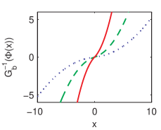
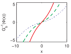
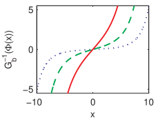
To compare the shrinkage properties of GPR and HPR we analyze select pairs of measurements in and . The derivation requires that is strongly concave on , strongly convex on and has gradient on . To see intuitively why this should hold for heavy-tailed marginals, note that for with fatter tails than a Gaussian, should eventually dominate . Figure 1 demonstrates graphically that the assumption holds for several choices of , provided is large enough, i.e., that has sufficiently heavy tails. Indeed, it can be shown that for scale parameters , the first and second derivatives of scale linearly with . Consider a measurement with . Analyzing such is relevant, as we are most interested in comparing how multiple reinforcing observations at clustered locations and a single isolated observation are absorbed during inference. By definition of , for we have as long as . The corresponding element then satisfies
| (8) |
Thus HPR inference leads to identical predictive distributions in -space at the two locations even though the isolated observation has disproportionately larger magnitude than , relative to the GPR measurements and . As this statement holds for any satisfying our earlier sign requirement, it indicates that HPR systematically shrinks isolated observations more strongly than GPR. Moreover, since the second derivative of scales linearly with an intuitive connection suggests itself when looking at inequality (8): the heavier the marginal tails, the stronger the inequality and thus the stronger the selective shrinkage.
The previous derivation exemplifies in an idealized setting that HPR leads to improved shrinkage of predictive distributions near isolated observations. More generally, because GPR transforms measurements only linearly, while HPR additionally pre-transforms measurements nonlinearly, our analysis suggests that for any GPR we can find an HPR model which leads to stronger selective shrinkage. The result has intuitive parallels to the parametric case: just as -regularization improves shrinkage of parametric estimators, heavy-tailed processes improve shrinkage of nonparametric estimators. Although our analysis kept fixed for GPR and HPR, in practice we are free to tune the kernel to yield a desired scale of predictive distributions. Lastly, although our analysis has been carried out for regression, it motivates us to explore heavy-tailed processes in the classification setting.
4 Heavy-tailed process classification
The derivation of our heavy-tailed process classifier (HPC) is similar to that of multiclass GPC with Laplace approximation in Section 3.5 of Rasmussen and Williams [12]. However, due to the nonlinear transformations involved, some nice properties of their derivation are lost. We revert notation and let denote a vector of class labels. For a -class classification problem with training points we introduce a vector of latent function measurements
For each block of variables we define an independent heavy-tailed process prior using Eq. (4) with a kernel matrix . Equivalently, we can define the prior jointly on by letting be a block-diagonal kernel matrix with blocks . Each kernel matrix is defined by a (possibly different) symmetric positive semidefinite kernel with its own set of parameters. The following construction relaxes the earlier condition that and instead views as just some nonlinear transformation with parameter . By this relaxation we effectively adopt Liu et al.’s [9] interpretation that Eq. (4) defines the copula. The scale parameters could in principle vary across the variables, but we keep them constant at least within each block of . Labels are represented in a 1-of- form and generated by the following observation model
| (9) |
For inference we are ultimately interested in computing
| (10) |
where . The previous section motivates the hope that improved selective shrinkage will occur in , provided the prior marginals have sufficiently heavy tails.
4.1 Inference
As in GPC, most of the intractability lies in computing the predictive distribution . We use the Laplace approximation to address this issue: a Gaussian approximation to is found and then combined with the Gaussian to give us an approximation to . This is then transformed to a (typically non-Gaussian) distribution in -space using a change of variables. Hence we first seek to find a mode and corresponding Hessian matrix of the log posterior . Recalling the relation , the log posterior can be written as
Let be an matrix of stacked diagonal matrices for -subvectors of . With , the gradients are
Unlike in Rasmussen and Williams [12], is not generally positive definite owing to its first term. For that reason we cannot use a Newton step to find the mode and instead resort to a simpler gradient method. Once the mode has been found we approximate the posterior as
and use this to approximate the predictive distribution by
Since we arranged for both distributions in the integral to be Gaussian, the resulting Gaussian can be straightforwardly evaluated. Finally, to approximate the one-dimensional integral with respect to in Eq. (10) we could either use a quadrature method, or generate samples from , convert them to -space using and then approximate the expectation by an average. We have compared predictions resulting using the latter method with those of a Gibbs sampler; the Laplace approximation matched Gibbs results well, while costing only a fraction of time to compute.
4.2 Parameter estimation
Using a derivation similar to that in section 3.4.4 of [12], we have for that the Laplace approximation of the marginal log likelihood is
| (11) | ||||
We optimize kernel parameters by taking gradient steps on . The derivative needs to take into account that perturbing the parameters can also perturb the mode found for the Laplace approximation. At an optimum must be zero, so that
| (12) |
where is defined as in Eq. (9) but using rather than . Taking derivatives of this equation allows us to compute the gradient . Differentiating the marginal likelihood we have
The remaining gradient computations are straightforward, albeit tedious. In addition to optimizing the kernel parameters, it may also be of interest to optimize the scale parameter of marginals . Again, differentiating Eq. (12) with respect to allows us to compute . We note that when perturbing we change by changing the underlying mode as well as by changing the parameter which is used to compute from . Suppressing the detailed computations, the derivative of the marginal log likelihood with respect to is
5 Experiments
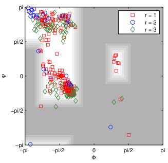
To a first approximation, the three-dimensional structure of a folded protein is defined by pairs of continuous backbone angles , one pair for each amino-acid, as well as discrete angles, so-called rotamers, that define the conformations of the amino-acid sidechains that extend from the backbone. The geometry is outlined in Figure 2. There is a strong dependence between backbone angles and rotamer values; this is illustrated in the “Ramachandran plot” shown in Figure 2, which plots the backbone angles for each rotamer (indicated by the shapes/colors). The dependence is exploited in computational approaches to protein structure prediction, where estimates of rotamer probabilities given backbone angles are used as one term in an energy function that models native protein states as minima of the energy. Protein structures are predicted by minimizing the energy function. Poor estimates of rotamer probabilities in sparse regions can derail the prediction procedure. Indeed, sparsity has been a serious problem in state-of-the-art rotamer models based on kernel density estimates (Roland Dunbrack, personal communication). Unfortunately, we have found that GPC is not immune to the sparsity problem.
To evaluate our algorithm we consider rotamer-prediction tasks on the 17 amino-acids (out of 20) that have three rotamers at the first dihedral angle along the sidechain222Residues ala and gly are non-discrete while pro has only two rotamers at the first dihedral angle.. Our previous work thus applies with the number of classes and the covariates being angle pairs. Since the input space is a torus we defined GPC and HPC using the following von Mises-inspired kernel for -dimensional angular data:
where and 333The function is a symmetric positive semi-definite kernel. By Propositions 3.22 (i) and (ii) and Proposition 3.25 in Shawe-Taylor and Cristianini [14], so is above.. To find good GPC kernel parameters we optimize an -regularized version of the Laplace approximation to the log marginal likelihood reported in Eq. 3.44 of [12]. For HPC we let be either the centered Laplace distribution or the hyperbolic secant distribution with scale parameter . We estimate HPC kernel parameters as well as by similarly maximizing an -regularized form of Eq. (11). In both cases we restricted the algorithms to training sets of only 100 datapoints. Since good regularization parameters for the objectives are not known a priori we train with and test them on a grid for each of the 17 rotameric residues in ten-fold cross-validation. To find good regularization parameters for a particular residue we look up that combination which, averaged over the ten folds of the remaining 16 residues, produced the best test results. Having chosen the regularization constants we report average test results computed in ten-fold cross validation.
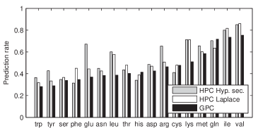
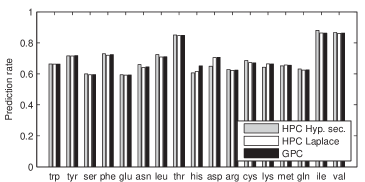
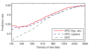
We evaluate the algorithms on predefined sparse and dense regions in the Ramachandran plot, as indicated by the background shading in Figure 2. Across 17 residues the sparse regions usually contained more than 70 measurements (and often more than 150), each of which appears in one of the 10 cross-validation folds. Figure 3 compares the label prediction rates on the dense and sparse regions. Averaged over all 17 residues HPC outperforms GPC by 5.79% with Laplace and 7.89% with hyperbolic secant marginals. With Laplace marginals HPC underperforms GPC on only two residues in sparse regions: by 8.22% on gln, and by 2.53% on his. On dense regions HPC lies within 0.5% on 16 residues and only degrades once by 3.64% on his. Using hyperbolic secant marginals HPC often improves GPC by more than 10% on sparse regions and degrades by more than 5% only on cys and his. On dense regions HPC usually performs within 1.5% of GPC. In Figure 4 we show how the average rotamer prediction rate across 17 residues changes as we grow the sparse region to include more measurements from dense regions. The growth of the sparse region is indicated by progressively lighter shadings in Figure 2. As more points are included the significant advantage of HPC lessens. Eventually GPC does marginally better than HPC. The values reported in Figure 3 correspond to the dark shaded region, which contains an average of 155 measurements per residue.
6 Related research
Copulas [10] allow convenient modelling of multivariate correlation structures as separate from marginal distributions. Early work by Song [16] used the Gaussian copula to generate complex multivariate distributions by complementing a simple copula form with marginal distributions of choice. Popularity of the Gaussian copula in the financial literature is generally credited to Li [8] who used it to model correlation structure for pairs of random variables with known marginals. More recently, the Gaussian process has been modified in a similar way to ours by Snelson et al. [15] who called the resulting stochastic process a Warped Gaussian Process. They demonstrate that posterior distributions can better approximate the true noise distribution if the transformation defining the warped process is learned. Jaimungal and Ng [7] have extended this work to model multiple parallel time series with marginally non-Gaussian stochastic processes under the name of Kernel-based Copula Processes (KCPs). Their work uses a “binding copula” to combine several subordinate copulas into a joint model. Bayesian approaches focusing on estimation of the Gaussian copula covariance matrix for a given dataset are given in [4, 11]. With the advent of larger datasets, research has also focused on estimation in high-dimensional settings. Liu et al. [9] do away with a prior on covariance matrices and give consistency results for a covariance estimator in high-dimensional settings.
7 Conclusions
This paper has analyzed learning scenarios where outliers are observed in the input space, rather than the output space as commonly discussed in the literature. We illustrated heavy-tailed processes as a straightforward extension of GPs and an elegant and economical way to improve the robustness of estimators in sparse regions beyond those of GP-based methods. This was demonstrated both by a theoretical analysis and experimental results. Importantly, because heavy-tailed processes are based on a GP, they inherit many of its favorable computational properties; predictive inference in regression, for instance, is straightforward. For approximate inference in more complicated models utilizing heavy-tailed processes, this paper exemplifies that we can borrow many ideas from standard GP models. Since heavy-tailed processes have a parsimonious representation, they can be easily used as building blocks in more complicated models where currently GPs are used. The benefits of heavy-tailed processes on selective shrinkage thus extend to many other GP-based models that currently struggle with covariate shift.
8 Acknowledgements
We would like to thank Roland Dunbrack and Maxim Shapovalov for helpful discussions and for giving us access to the data.
References
- [1] Tamara Broderick and Robert B. Gramacy. Classification and Categorical Inputs with Treed Gaussian Process Models. 2009.
- [2] Wei Chu and Zoubin Ghahramani. Gaussian Processes for Ordinal Regression. Journal of Machine Learning Research, 6:2005, 2004.
- [3] Doris Damian, Paul D. Sampson, and Peter Guttorp. Bayesian Estimation of Semi-Parametric Non-Stationary Spatial Covariance Structures. Environmetrics, 12:161–178.
- [4] Adrian Dobra and Alex Lenkoski. Copula Gaussian Graphical Models. Technical report, 2009.
- [5] Paul W. Goldberg, Christopher K. I. Williams, and Christopher M. Bishop. Regression with Input-dependent Noise: A Gaussian Process Treatment. In In Advances in Neural Information Processing Systems 10, pages 493–499. MIT Press, 1998.
- [6] Robert B. Gramacy and Herbert K. H. Lee. Bayesian Treed Gaussian Process Models with an Application to Computer Modeling. Journal of the American Statistical Association, 2007.
- [7] Sebastian Jaimungal and Eddie K. Ng. Kernel-based Copula Processes. In ECML PKDD ’09: Proceedings of the European Conference on Machine Learning and Knowledge Discovery in Databases, pages 628–643, Berlin, Heidelberg, 2009. Springer-Verlag.
- [8] David X. Li. On Default Correlation: A Copula Function Approach. Technical Report 99-07, Riskmetrics Group, New York, April 2000.
- [9] Han Liu, John Lafferty, and Larry Wasserman. The Nonparanormal: Semiparametric Estimation of High Dimensional Undirected Graphs. Journal of Machine Learning Research, 10:1–37, 2009.
- [10] Roger B. Nelsen. An Introduction to Copulas. Springer, 1999.
- [11] Michael Pitt, David Chan, and Robert J. Kohn. Efficient Bayesian Inference for Gaussian Copula Regression Models. Biometrika, 93(3):537–554, 2006.
- [12] Carl E. Rasmussen and Christopher K. I. Williams. Gaussian Processes for Machine Learning. MIT Press, 2006.
- [13] Alexandra M. Schmidt and Anthony O’Hagan. Bayesian Inference for Nonstationary Spatial Covariance Structure via Spatial Deformations. Journal of the Royal Statistical Society, 65(3):743–758, 2003. Ser. B.
- [14] John Shawe-Taylor and Nello Cristianini. Kernel Methods for Pattern Analysis. Cambridge University Press, New York, NY, USA, 2004.
- [15] Ed Snelson, Carl E. Rasmussen, and Zoubin Ghahramani. Warped Gaussian Processes. volume 16, pages 337–344. NIPS, 2004.
- [16] Peter Xue-Kun Song. Multivariate Dispersion Models Generated From Gaussian Copula. Scandinavian Journal of Statistics, 27(2):305–320, 2000.