Competing orders in the generalized Hund chain model at half-filling

Abstract

By using a combination of several non-perturbative techniques – a one-dimensional field theoretical approach together with numerical simulations using density matrix renormalization group – we present an extensive study of the phase diagram of the generalized Hund model at half-filling. This model encloses the physics of various strongly correlated one-dimensional systems, such as two-leg electronic ladders, ultracold degenerate fermionic gases carrying a large hyperfine spin $\frac{3}{2}$, other cold gases like Ytterbium 171 or alkaline-earth condensates. A particular emphasis is laid on the possibility to enumerate and exhaust the eight possible Mott insulating phases by means of a duality approach. We exhibit a one-to-one correspondence between these phases and those of the two-leg electronic ladders with interchain hopping. Our results obtained from a weak coupling analysis are in remarkable quantitative agreement with our numerical results carried out at moderate coupling.

I Introduction

A major focus of the study of strongly correlated electronic systems is the analysis of the competition between qualitatively distinct ground states and the associated quantum phase transitions (QPT) sachdev in low dimensions. A reason to concentrate on these matters stems from the hope that the criticality of the system at such QPT’s possibly results in a universal description of their vicinity. In $2+1$ space-time dimensions, the resulting relativistic quantum field theories which describe the zero-temperature transition between these quantum phases are in general strongly coupled and can be highly non-trivial senthil .

In one dimension, the situation is much simpler since the quantum critical points in standard condensed matter systems are characterized by conformal field theories (CFT), which often admit a simple free-field representation in terms of free bosons or fermions. In this respect, the bosonization approach has been very successful to investigate the physical properties of one-dimensional quantum phases bookboso ; giamarchi . Within this approach, several conventional and exotic long-range ordered phases have been revealed over the years in two-leg ladder models Linso8 ; szh ; frahm ; lehur ; marston1 ; marston2 ; furusaki ; wu04 ; momoi ; assarafdemirep ; fabrizio ; Lee ; marston3 ; bunder and carbon nanotube systems linCarbone ; nersesyan03 ; nersesyan07 ; bunder08 at half-filling. Two different classes of Mott-insulating phases have been found at half-filling in these systems. A first class is two-fold degenerate corresponding to the spontaneous breaking of discrete symmetries such as the translation symmetry in charge density wave (CDW) and bond-ordering phases, or the time-reversal symmetry in d-density wave (DDW) phase. In contrast, the second class of Mott-insulating phases is non-degenerate. A paradigmatic example of this class is the Haldane phase of the spin-1 Heisenberg chain haldane and of the two-leg spin ladder which breaks spontaneously a non-local Z₂ $\times$ Z₂ discrete symmetry tasaki ; shelton ; string2leg .

Another striking particularity of many one-dimensional electronic systems is the existence of hidden duality symmetries, within the low-energy approach, which relate many of the competing orders to a conventional one like the CDW Linso8 ; schulz ; momoi ; lee ; controzzi ; totsuka ; boulat . Actually, a general duality approach has been introduced recently to describe the zero-temperature spin-gapped phases of one-dimensional (1D) electronic systems away from half-filling boulat . In this paper, we apply this approach to half-filled systems of four-component fermions and revisit the problem of competing orders in half-filled two-leg electronic ladders. In this particular case, some of the duality symmetries already exist at the level of the lattice model, and have been first revealed in Ref. momoi, . In addition to these, as it will be seen, there are also interesting emergent duality symmetries which relate non-degenerate Mott insulating phases to conventional order such as CDW. Unlike the former ones, those dualities do not bear a local representation on the lattice.

The starting point of the duality approach to competing orders is to identify the internal global symmetry group H of the lattice model. For two-leg electronic ladders, or more generally two-band models, the building blocks of the model are four-component fermionic creation operators on each site $i$: $c^{{\dagger}}_{l\sigma,i}$ where $l=1,2$ is the leg or orbital index and $\sigma=\uparrow,\downarrow$ denotes the spin-$\frac{1}{2}$ index. Three basic global continuous symmetries are retained: a U(1) charge symmetry ($c_{l\sigma,i}\rightarrow e^{i\phi}c_{l\sigma,i}$), a SU(2) spin-rotational invariance ($c_{l\sigma,i}\rightarrow\sum_{\sigma^{{}^{\prime}}}(e^{i{\vec{\theta}}\cdot{\vec{\sigma}}/2})_{\sigma\sigma^{{}^{\prime}}}c_{l\sigma^{{}^{\prime}},i}$, ${\vec{\sigma}}$ being the Pauli matrices), and a U(1) orbital symmetry ($c_{1(2)\sigma,i}\rightarrow e^{\pm i\phi}c_{1(2)\sigma,i}$). Moreover, we will consider models for which the two legs, or two bands behave identically; in other words, we impose a Z₂ invariance under the permutation of the legs. If we restrict ourselves to on-site interactions, the most general model with H $=$ U(1)_c $\times$ SU(2)_s $\times$ U(1)_o $\times$ Z₂ invariance then reads as follows arovas :

$$\mathcal{H} = -t\sum_{i,l\sigma}\left(c^{\dagger}_{l\sigma,i}c^{\phantom{{\dagger}}}_{l\sigma,i+1}+\mbox{h.c.}\right)-\mu\sum_{i}n_{i}+\frac{U}{2}\sum_{i}n_{i}^{2}$$ (1)

$$+ J_{H}\sum_{i}\vec{S}_{1,i}\cdot\vec{S}_{2,i}+J_{t}\sum_{i}(T_{i}^{z})^{2},$$

with $n_{i}=\sum_{l\sigma}n_{l\sigma,i}$ ($n_{l\sigma,i}=c^{{\dagger}}_{l\sigma,i}c_{l\sigma,i}^{\vphantom{\dagger}}$) being the occupation number on the $i^{\mbox{\scriptsize th}}$ site. In Eq. (1), the spin operator on leg $l$ is defined by

$$\vec{S}_{l,i}=\frac{1}{2}\sum_{\alpha,\beta}c_{l\alpha,i}^{\dagger}\vec{\sigma}_{\alpha\beta}c^{\phantom{{\dagger}}}_{l\beta,i},$$ (2)

whereas $T_{i}^{z}=\frac{1}{2}\sum_{\sigma}(n^{\phantom{{\dagger}}}_{1\sigma,i}-n^{\phantom{{\dagger}}}_{2\sigma,i})$ is the generator of the U(1) symmetry for orbital degrees of freedom.

Model (1) depends on three microscopic couplings: a Coulombic interaction $U$, a Hund coupling $J_{H}$, and an “orbital crystal field anisotropy” $J_{t}$. When $J_{t}=0$, the resulting model is the so-called Hund model which has been investigated in the context of orbital degeneracy arovas ; lee ; fabrizio . The generalized Hund model (1) is directly linked to ultracold fermionic ¹⁷¹Yb and alkaline-earth atoms with nuclear spin $I=\frac{1}{2}$ fukuhara ; gorshkov . The two-orbital states are described in these systems by the ground state (¹S₀ $\equiv$ g) and a long-lived excited state (³P₀ $\equiv$ e). The almost perfect decoupling of the nuclear spin from the electronic angular momentum $J$ in the two $e,g$ states ($J=0$ states) makes the s-wave scattering lengths of the problem independent of the nuclear spin. The low-energy Hamiltonian relevant to the ¹⁷¹Yb cold gas loaded into a 1D optical lattice then reads gorshkov :

$${\cal H}_{\rm Yb} = -t\sum_{i,l\sigma}\left(c^{\dagger}_{l\sigma,i}c^{\phantom{{\dagger}}}_{l\sigma,i+1}+\mbox{h.c.}\right)+\frac{{\tilde{U}}}{2}\sum_{i,l}n_{l,i}(n_{l,i}-1)$$ (3)

$$+ V\sum_{i}n_{g,i}n_{e,i}+V_{ex}\sum_{i,\alpha,\beta}c^{\dagger}_{g\alpha,i}c^{\dagger}_{e\beta,i}c_{g\beta,i}^{\vphantom{\dagger}}c_{e\alpha,i}^{\vphantom{\dagger}},$$

where $c^{\dagger}_{l\sigma,i}$ is the fermionic creation operator at site $i$ with the nuclear spin-$\frac{1}{2}$ index $\sigma=\uparrow,\downarrow$ in the $l=e,g$ electronic states. The occupation number of electronic states is $n_{l,i}=\sum_{\sigma}c^{{\dagger}}_{l\sigma,i}c_{l\sigma,i}^{\vphantom{\dagger}}$. Model (3) is then directly equivalent to the generalized Hund model (1) with the correspondence: ${\tilde{U}}=U+J_{t}/2$, $V=U-J_{t}/2-J_{H}/4$, and $V_{ex}=-J_{H}/2$.

Apart from this connection to cold fermions physics, one of the main interests of model (1) stems from the fact that it contains a large variety of relevant models with extended continuous symmetries, some of which having appeared in different contexts. First of all, when $J_{t}=-3J_{H}/4$, the continuous symmetry is promoted to U(1)_c $\times$ SU(2)_s $\times$ SU(2)_o, and one recovers the so-called spin-orbital model yamashita ; khomskii ; mila ; aza4spin ; itoi00 . In absence of Hund coupling, i.e., $J_{H}=0$, the continuous symmetry group of model (1) is U(1)_c $\times$ U(1)_o $\times$ SO(4)_s where each chain has a separate SU(2) spin-rotational symmetry. When $J_{t}=J_{H}/4$, model (1) displays an SO(5) symmetry which unifies spin and orbital degrees of freedom. The resulting model, with U(1)_c $\times$ SO(5)_s,o continuous symmetry, is relevant to four-component fermionic cold atom systems zhang ; Lecheminant2005 ; Wu2005 ; tsvelik06 ; tu ; wu06 ; sylvainquart ; capponiMS ; roux ; jiang ; heloise . Finally, when $J_{H}=J_{t}=0$, one recovers the U(4) Hubbard model, that has been extensively analyzed in recent years assarafdemirep ; assaraf ; solyom ; ueda . As it will be seen in Section II, at half-filling, many other highly symmetric lines can be identified. For instance, the line $J_{H}=8U$ unifies spin and charge degrees of freedom with an extended U(1)_o $\times$ SO(5)_s,c continuous symmetry sylvainzhang . The corresponding model has been previously introduced by Scalapino, Zhang and Hanke (SZH) szh in connection to the SO(5) theory which relates antiferromagnetism to d-wave superconductivity zhangso5 .

In this paper, we will investigate the nature of the insulating phases of the zero-temperature phase diagram of model (1) at half-filling. In this respect, it will be shown that the duality approach of Ref. boulat, for half-filled fermions with internal global symmetry group H = U(1)_c $\times$ SU(2)_s $\times$ U(1)_o $\times$ Z₂ yields eight fully gapped phases. These eight Mott-insulating phases fall into two different classes. On the one hand, the first class consists of four doubly degenerate phases which spontaneously break a discrete symmetry of the underlying lattice model. On the other hand, the second class contains four non-degenerate Mott insulating phases. A first one is the rung-singlet (RS) phase where two spins on each rung lock into a singlet. A second non-degenerate phase is a rung-triplet (RT) phase where the spins now combine into a triplet and this phase is known to be adiabatically connected to the Haldane phase of the spin-1 Heisenberg chain string2leg . Finally, two other Haldane-like phases are found: they are spin-singlet but involve two different pseudo-spin 1 operators which are respectively built from charge and orbital degrees of freedom. In the case of the charge pseudo-spin 1 operator, the resulting Haldane charge (HC) phase has been found very recently in the context of 1D half-filled spin-$\frac{3}{2}$ cold fermions heloise .

In addition to this duality approach, it will be shown, by means of a one-loop renormalization group (RG) approach and numerical simulations (using the Density Matrix Renormalization Group (DMRG) algorithm DMRG ), that the zero-temperature phase diagram of model (1) displays seven out of the eight expected insulating phases. We find it remarkable that model (1), that only has three independent coupling constants, turns out to have a rich phase diagram which includes the four non-degenerate Mott insulating phases.

Finally, we will make contact with the eight Mott-insulating phases found over the years in half-filled generalized two-leg ladders with a $t_{\perp}$ transverse hopping term furusaki ; wu04 . The latter term breaks explicitly the U(1)_o symmetry but it is known that this symmetry is recovered at low-energy Linso8 ; wu04 . The relevant global symmetry group is still H and the same duality approach thus applies to that case. In this respect, we will connect the two families of eight fully gapped phases found for $t_{\perp}=0$ and for $t_{\perp}\neq 0$. In particular, it will be shown that the two problems are in fact connected by an emergent non-local duality symmetry.

The rest of the paper is organized as follows. In Section II, we discuss the symmetries of model (1). We also present a strong-coupling analysis along special highly-symmetric lines which gives some clues about the nature of the non-degenerate Mott-insulating phases. The low-energy investigation is then presented in Section III. It contains the duality approach to half-filled fermions with internal symmetry group H $=$ U(1)_c $\times$ SU(2)_s $\times$ U(1)_o $\times$ Z₂. The zero-temperature phase diagram of the generalized Hund model (1) and that of highly symmetric models are deduced by a one-loop RG analysis. We then connect our results to the known insulating phases of generalized two-leg ladder models with a $t_{\perp}$ hopping term. In Section IV, we map out the phase diagram of model (1), SZH, and spin-orbital models with $t_{\perp}=0$ by means of DMRG calculations to complement the low-energy approach. Our concluding remarks are presented in Section V. The paper is supplied with three appendices which provide some additional information. Appendix A describes the technical details of the continuum limit of model (1). The low-energy approach of edge states in the non-degenerate Mott-insulating phases are discussed in Appendix B. Finally, Appendix C presents the main effect of the interchain hopping in the strong-coupling regime, close to the orbital symmetric line.

II Symmetries and strong coupling

Before investigating the zero-temperature phase diagram of the generalized Hund model by means of the low-energy and DMRG approaches, it is important to fully determine the special lines which exhibit enlarged symmetry. It turns out that, at half-filling, many highly symmetric lines can be highlighted. Their study will give some important clues on the possible Mott-insulating phases of the model at half-filling.

II.1 Highly symmetric lines

The generalized Hund model (1) enjoys a global internal symmetry group H $=$ U(1)_c $\times$ SU(2)_s $\times$ U(1)_o $\times$ Z₂ on top of the lattice discrete symmetries like one-step translation invariance, time-reversal symmetry, site and link parities. For generic filling, and on four different manifolds – that correspond to some fine-tuning of the lattice couplings – in the space of coupling constants, this model possesses a higher symmetry.

First of all, on top of the SU(2)_s that rotates spin degrees of freedom, one can define a SU(2)_o orbital pseudo-spin operator:

$$T_{i}^{\dagger} = c_{1\uparrow,i}^{\dagger}c_{2\uparrow,i}^{\vphantom{\dagger}}+c_{1\downarrow,i}^{\dagger}c_{2\downarrow,i}^{\vphantom{\dagger}}$$

$$T_{i}^{z} = \frac{1}{2}\left(n_{1,i}-n_{2,i}\right),$$ (4)

with $n_{l,i}=\sum_{\sigma}n_{l\sigma,i}$, $l=1,2$. When $J_{t}=-3J_{H}/4$, the U(1) orbital symmetry of the Hund model (1) is enlarged to SU(2)_o, with generators given by Eq. (4). The resulting model displays a U(1)_c $\times$ SU(2)_s $\times$ SU(2)_o continuous symmetry and has been considered in systems with orbital degeneracy like the spin-orbital model arovas ; yamashita ; khomskii ; mila ; aza4spin ; itoi00 .

A second highly symmetric model is defined for $J_{H}=0$: then the interacting part of model (1) simplifies as follow:

$${\cal H}^{\rm int}_{SO(4)} = \frac{1}{2}\left(U+\frac{J_{t}}{2}\right)\sum_{i}\left(n_{1,i}^{2}+n_{2,i}^{2}\right)$$ (5)

$$+ \left(U-\frac{J_{t}}{2}\right)\sum_{i}n_{1,i}n_{2,i},$$

from which we deduce that each leg has a separate SU(2) spin rotation symmetry so that the continuous symmetry group of model (5) is U(1)_c $\times$ U(1)_o $\times$ SO(4)_s.

When $J_{t}=J_{H}/4$, as shown in Ref. sylvainzhang, , model (1) is known to be equivalent to the spin-$\frac{3}{2}$ cold fermionic model with interacting part:

$${\cal H}^{\rm int}_{{\rm spin-}\frac{3}{2}}=U_{0}\sum_{i}P^{\dagger}_{00,i}P_{00,i}^{\vphantom{\dagger}}+U_{2}\sum_{i}\sum_{m=-2}^{2}P^{\dagger}_{2m,i}P_{2m,i}^{\vphantom{\dagger}},$$ (6)

where $U_{0}=(2U-7J_{t})/4$, and $U_{2}=(2U+J_{t})/4$. In Eq. (6), we have $P^{\dagger}_{Jm,i}=\sum_{\alpha\beta}\langle{Jm|\frac{3}{2},\frac{3}{2};\alpha\beta}\rangle c^{\dagger}_{\alpha,i}c^{\dagger}_{\beta,i}$, $\alpha,\beta=\pm\frac{3}{2},\pm\frac{1}{2}$, and $\langle{Jm|\frac{3}{2},\frac{3}{2};\alpha\beta}\rangle$ are the Clebsch-Gordan coefficients for spin $\frac{3}{2}$. Model (6) is known to exhibit a U(1)_c $\times$ SO(5)_s,o continuous symmetry without any fine-tuning zhang .

Finally, for $J_{H}=J_{t}=0$, spin and orbital degrees of freedom unify to a maximal SU(4) symmetry and model (1) takes the form of the Hubbard model for four component fermions with a U(4) invariance.

At half-filling, the chemical potential $\mu$ is given by $\mu_{0}=\frac{3U}{2}$ to ensure particle-hole symmetry. More highly-symmetric lines can be found in this particle-hole symmetric case. It stems from the fact that, as in the spin-$\frac{1}{2}$ Hubbard model, the U(1)_c charge symmetry can be enlarged to an SU(2)_c symmetry at half-filling yang ; yangzhang . In this respect, one can define a charge pseudo-spin operator by:

$$J_{i}^{\dagger} = c_{1\uparrow,i}^{\dagger}c_{2\downarrow,i}^{{\dagger}}-c_{1\downarrow,i}^{\dagger}c_{2\uparrow,i}^{{\dagger}}$$

$$J_{i}^{z} = \frac{1}{2}\left(n_{i}-2\right),$$ (7)

which is a SU(2)_s spin-singlet that satisfies the SU(2) commutation relations. This operator is the generalization in two-leg ladder or two-band systems of the pseudo-spin $\frac{1}{2}$ operator introduced by Andersonanderson and by Yang in eta-pairing problems yang .

Many interesting lines can then be considered. A simple way to reveal them is to consider the energy levels of the one-site Hamiltonian (1) with $t=0$. The corresponding spectrum is depicted in Fig. 1. On top of the four symmetric lines that we have identified above, we find nine additional lines where higher continuous symmetries emerge (see Table 1). Among all these new highly symmetric lines, there are three interesting models with two independent coupling constants, i.e., with only one fine-tuning.

Figure 1: Energy level diagram for the one-site Hamiltonian (1) with $t=0$.

Table 1: Extended continuous symmetries of model (1) at half-filling

Extended continuous symmetry	Fine-tuning	Degenerate levels
$U(1)_{c}\times SU(2)_{o}\times SU(2)_{s}$	$J_{t}=-3J_{H}/4$	$E_{2}=E_{4}$
$U(1)_{c}\times U(1)_{o}\times SO(4)_{s}$	$J_{H}=0$	$E_{3}=E_{4}$
$U(1)_{c}\times SO(5)_{s,\,o}$	$J_{t}=J_{H}/4$	$E_{2}=E_{3}$
$U(1)_{c}\times SU(4)_{s,\,o}$	$J_{H}=J_{t}=0$	$E_{2}=E_{3}=E_{4}$
$SO(7)$	$J_{t}=2U,\,J_{H}=8U$	$E_{0}=E_{2}=E_{3}$
$U(1)_{o}\times SU(4)_{s,\,c}$	$U=J_{H}=0$	$E_{0}=E_{3}=E_{4}$
$SU(2)_{c}\times SO(5)_{s,\,o}$	$J_{t}=-2U/3,\,J_{H}=-8U/3$	$E_{0}=E_{4},\,E_{2}=E_{3}$
$SU(2)_{o}\times SO(5)_{s,\,c}$	$J_{t}=-6U,\,J_{H}=8U$	$E_{0}=E_{3},\,E_{2}=E_{4}$
$SO(5)_{c,\,o}\times SU(2)_{s}$	$J_{t}=2U,\,J_{H}=-8U/3$	$E_{0}=E_{2}=E_{4}$
$U(1)_{o}\times SO(5)_{s,\,c}$	$J_{H}=8U$	$E_{0}=E_{3}$
$SO(4)_{c,\,o}\times SO(4)_{s}$	$J_{H}=0,\,J_{t}=2U$	$E_{0}=E_{2},\,E_{3}=E_{4}$
$SO(4)_{c,\,o}\times SU(2)_{s}$	$J_{t}=2U$	$E_{0}=E_{2}$
$U(1)_{o}\times SU(2)_{s}\times SU(2)_{c}$	$J_{H}=-8U/3$	$E_{0}=E_{4}$

A first one corresponds to the SZH model with U(1)_o $\times$ SO(5) continuous symmetry. Such SZH model with no transversal hopping $t_{\perp}$ is defined as follows: $\mathcal{H}_{\rm SZH}=\mathcal{H}_{t_{\parallel}}+\mathcal{H}_{\textrm{rung}}$ with

$$\mathcal{H}_{t_{\parallel}}=-t\sum_{i,\,\sigma}(c_{\sigma,\,i}^{\dagger}c_{\sigma,\,i+1}^{\vphantom{\dagger}}+d_{\sigma,\,i}^{\dagger}d_{\sigma,\,i+1}^{\vphantom{\dagger}}+\mbox{h.c.}),$$

$$\mathcal{H}_{\textrm{rung}}=U_{\textrm{SZH}}\sum_{i}\left((n^{\phantom{{\dagger}}}_{c\uparrow,\,i}-\frac{1}{2})(n^{\phantom{{\dagger}}}_{c\downarrow,\,i}-\frac{1}{2})+(c\rightarrow d)\right)$$

$$\qquad+V_{\textrm{SZH}}\sum_{i}(n^{\phantom{{\dagger}}}_{c,\,i}-1)(n^{\phantom{{\dagger}}}_{d,\,i}-1)$$

$$\qquad+J_{\textrm{SZH}}\sum_{i}\vec{S}_{c,\,i}\cdot\vec{S}_{d,\,i},$$ (8)

where $c_{\sigma}$ and $d_{\sigma}$ are respectively the fermion annihilation operator of the upper and lower leg of the ladder with spin index $\sigma$. The occupation numbers on the $i^{\mbox{\scriptsize th}}$ site are denoted by $n_{c(d),i}$ respectively. The spin operators ${\vec{S}}_{c(d),i}$ are defined similarly to those of the Hund model (see Eq. (2)). It is straightforward to relate the SZH model to the generalized Hund model (1):

$$U=\frac{U_{SZH}+V_{SZH}}{2}$$

$$J_{H}=J_{SZH}$$

$$J_{t}=U_{SZH}-V_{SZH}.$$ (9)

As shown in Ref. szh, , the fine-tuning $J_{\textrm{SZH}}=4(U_{\textrm{SZH}}+V_{\textrm{SZH}})$ (i.e., $J_{H}=8U$ in the context of model (1)) makes the lattice model (8) U(1)_o $\times$ SO(5)_s,c symmetric. The SO(5) symmetry unifies here spin and charge degrees of freedom and is thus different from the spin-$\frac{3}{2}$ cold fermionic atoms (6) case.

A second symmetric line is found for $J_{t}=2U$ with the emergence of a SU(2)_s $\times$ SO(4)_c,o continuous symmetry. In that case, charge and orbital degrees of freedom play a symmetric role and are unified by a SO(4) symmetry.

Finally, the last extended symmetric ray with the fine-tuning $J_{H}=-8U/3$ (see Table I) corresponds to a model with U(1)_o $\times$ SU(2)_c $\times$ SU(2)_s continuous symmetry. Such a model has two independent SU(2) symmetries: one for the spin degrees of freedom and also a second for the charge degrees of freedom. In this respect, it is very similar to the spin-orbital model and can be called “charge-spin” model.

II.2 Strong-coupling analysis

The identification of these highly symmetric models is very useful since several possible insulating phases of the generalized Hund model (1) can be inferred from a strong-coupling analysis. Such an approach has already been performed for some special lines of Table I such as the half-filled U(4) Hubbard chain affleckmarston ; onufriev , the SO(5) spin-$\frac{3}{2}$ model wu06 ; heloise , and the SZH one szh ; frahm .

Here, we present a simple strong-coupling approach along three special lines which enables us to identify several non-degenerate Mott-insulating phases. To this end, let us first consider the line $J_{t}=2U$ with $U>0$ and $J_{H}<0$. In the absence of hopping term (i.e., $t=0$), the lowest energy states are the spin triplet $E_{3}$ (see Fig. 1). An effective Hamiltonian can then be deduced by treating the hopping term as a perturbation in the strong coupling regime $|U,J_{H},J_{t}|\gg t$. At second order of perturbation theory, we find an antiferromagnetic SU(2) Heisenberg chain:

$$\mathcal{H}_{\text{eff}}=J_{s}\sum_{i}\left(\vec{S}_{1,i}+\vec{S}_{2,i}\right)\cdot\left(\vec{S}_{1,i+1}+\vec{S}_{2,i+1}\right),$$ (10)

where $J_{s}=-4t^{2}/(J_{H}-4U)>0$, and $\vec{S}_{l,i}$ are the spin operators defined in Eq. (2). The resulting fully gapped phase is the well-known RT phase of the two-leg spin-$\frac{1}{2}$ ladder which is adiabatically connected to the Haldane phase of the spin-1 chain string2leg . Such a non-degenerate gapful phase displays a hidden antiferromagnetic ordering which is revealed by a string-order parameter dennijs ; shelton ; kim :

$$\lim_{|i-j|\rightarrow\infty}\langle\left(S^{z}_{1,i}+S^{z}_{2,i}\right)e^{i\pi\sum_{k=i+1}^{j-1}\left(S^{z}_{1,k}+S^{z}_{2,k}\right)}$$

$$\times\left(S^{z}_{1,j}+S^{z}_{2,j}\right)\rangle\neq 0.$$ (11)

This RT phase is also known to exhibit spin-$\frac{1}{2}$ edge states when open-boundary conditions are considered aklt ; kennedy ; orignac .

A second interesting line is $J_{H}=-8U/3$ where the charge degrees of freedom enjoy an SU(2) symmetry enlargement. In the absence of hopping term, the lowest energy states for $U<0$ and $J_{t}>0$ are the $E_{0},E_{4}$ levels as it can be seen from Fig. 1. Keeping only these three states, we obtain, at second order of perturbation theory, an effective (pseudo) spin-1 antiferromagnetic SU(2) Heisenberg chain:

$$\mathcal{H}_{\text{eff}}=J_{c}\sum_{i}\vec{J}_{i}\cdot\vec{J}_{i+1},$$ (12)

with $J_{c}=-4t^{2}/(6U-J_{t})>0$. The effective Hamiltonian (12) expresses in terms of the spin-singlet charge operator (7) which is a pseudo spin-1 operator in the triplet states $E_{0},E_{4}$ of Fig. 1. We then expect the emergence of Haldane-like phase for charge degrees of freedom as it has been recently found in the context of half-filled spin-$\frac{3}{2}$ cold fermions heloise . Such a HC phase is fully gapped and non-degenerate. It displays a hidden ordering that is revealed by the string-order parameter:

$$\lim_{|i-j|\rightarrow\infty}\langle J^{z}_{i}e^{i\pi\sum_{k=i+1}^{j-1}J^{z}_{k}}J^{z}_{j}\rangle\neq 0.$$ (13)

A deviation from the line $J_{H}=-8U/3$ breaks the SU(2) charge symmetry down to U(1) and in the strong-coupling regime the lowest correction to model (12) is a single-ion anisotropy term $D_{c}\sum_{i}(J_{i}^{z})^{2}$ (with $D_{c}=3J_{H}/4+2U$). The Haldane phase of the spin-1 chain is known to be stable under a weak single-ion anisotropy schulzspin1 . A large enough $D_{c}$ may give rise to a Ising phase with $\langle J^{z}_{i}\rangle\neq 0$ (i.e. a CDW from the definition (7)) or to a large-$D_{c}$ phase which is a non-degenerate gapped singlet phase. The latter, with $\langle J^{z}_{i}\rangle=0$, corresponds to the RS phase of the two-leg spin-$\frac{1}{2}$ ladder where the two spins of the rung bind into a singlet state ($E_{4}$ state of Fig. 1) for an antiferromagnetic interchain coupling.

Finally, a last interesting symmetric ray is $J_{t}=-3J_{H}/4$ where the U(1) orbital symmetry is enlarged to SU(2). Along this line, when $J_{H}>0$ and $U$ is not too negative, the lowest energy states of the one-site Hamiltonian are levels $E_{2},E_{4}$ of Fig. 1. At second order of perturbation theory, we now find a spin-1 antiferromagnetic SU(2) Heisenberg chain for the orbital degrees of freedom:

$$\mathcal{H}_{\text{eff}}=J_{o}\sum_{i}\vec{T}_{i}\cdot\vec{T}_{i+1},$$ (14)

with $J_{o}=16t^{2}/(9J_{H}+8U)$. We thus expect the emergence of a new Haldane phase for the orbital degrees of freedom that will be called Haldane orbital (HO) phase in the rest of the paper. The resulting hidden ordering is captured by the following string-order parameter:

$$\lim_{|i-j|\rightarrow\infty}\langle T^{z}_{i}e^{i\pi\sum_{k=i+1}^{j-1}T^{z}_{k}}T^{z}_{j}\rangle\neq 0.$$ (15)

A deviation from the line $J_{t}=-3J_{H}/4$ breaks the SU(2) orbital symmetry down to U(1) and in the strong-coupling regime the lowest correction to model (14) is a single-ion anisotropy term $D_{o}\sum_{i}(T_{i}^{z})^{2}$ (with $D_{o}=J_{t}+3J_{H}/4$). For sufficiently strong value of $|D_{o}|$, the HO phase will be destabilized into either an orbital density wave (ODW) which is described by the $E_{2}$ states with $\langle T_{i}^{z}\rangle\neq 0$ or a RS phase, i.e., the $E_{4}$ state with $\langle T_{i}^{z}\rangle=0$.

In summary, the strong-coupling analysis along highly symmetric lines reveals the existence of four non-degenerate Mott-insulating phases (RT, HC, HO, RS) and two gapful phases with long-range density ordering (CDW, ODW).

III Low-energy Approach

In this section, we present the details of the low-energy approach of the generalized Hund model (1) at half-filling, in the weak-coupling regime $|U,J_{H},J_{t}|\ll t$. The zero-temperature phase diagram of model (1) will be investigated by means of the combination of a duality approach and one-loop RG calculations. In particular, we will determine the different insulating phases in the weak-coupling regime and make connection with the ones found within the strong-coupling approach.

III.1 Phenomenological approach

The starting point of the low-energy approach is the linearization around the Fermi points $\pm k_{F}$ of the dispersion relation for non-interacting four-component fermions. We thus introduce four left and right moving Dirac fermions $L_{l\sigma},R_{l\sigma}$ ($l=1,2$ and $\sigma=\uparrow,\downarrow$), which describe the lattice fermions $c_{l\sigma,i}$ in the continuum limit:

$$\frac{c^{\phantom{{\dagger}}}_{l\sigma,i}}{\sqrt{a_{0}}}\to R_{l\sigma}(x)e^{ik_{F}x}+L_{l\sigma}(x)e^{-ik_{F}x},$$ (16)

with $k_{F}=\pi/2a_{0}$ at half-filling and $x=ia_{0}$ ($a_{0}$ being the lattice spacing). The next step of the approach is to use the Abelian bosonization of these Dirac fermions to obtain the low-energy effective Hamiltonian for model (1). The details of these calculations are given in Appendix A. Here, we present a more phenomenological approach which is based on the symmetries of the lattice model (1).

The continuous symmetry of the non-interacting model (1) is SO(8). In the continuum limit, the SO(8) symmetry can be revealed by introducing eight real (Majorana) fermions from the four complex Dirac $(R,L)_{l\sigma}$ ones. The non-interacting fixed point is then described by the SO(8)₁ CFT with central charge $c=4$ dms . The chiral currents $J_{L,R}^{(a,b)}$ ($1\leq a<b\leq 8$), which generates this CFT, can be expressed as fermionic bilinears: $J_{L(R)}^{(a,b)}=i\xi^{a}_{L(R)}\xi^{b}_{L(R)}$, where $\xi^{a}_{L(R)}$ are the eight left (right) moving Majorana fermions.

When interactions are included, the SO(8) symmetry is broken down to H $=$ U(1)_c $\times$ SU(2)_s $\times$ U(1)_o $\times$ Z₂. The key point of the analysis is to identify how the eight Majorana fermions of the SO(8)₁ CFT act in H. One way to obtain the correspondence is to focus on the currents which generate the different continuous symmetry groups in H. The uniform part of the continuum limit of the spin operator (2) on the leg $l=1,2$ defines the chiral SU(2)₁ currents ${\vec{J}}_{lR,L}$:

$${\vec{J}}_{lL}=L^{\dagger}_{l\alpha}\frac{{\vec{\sigma}}_{\alpha\beta}}{2}L_{l\beta}^{\vphantom{\dagger}},{\vec{J}}_{lR}=R^{\dagger}_{l\alpha}\frac{{\vec{\sigma}}_{\alpha\beta}}{2}R_{l\beta}^{\vphantom{\dagger}}.$$ (17)

As in two-leg spin ladder shelton ; allen , the sum and difference of these chiral SU(2)₁ currents can be locally expressed in terms of four Majorana fermions $\xi^{1,2,3,6}_{R,L}$ among the eight original ones:

$${\vec{J}}_{1R,L}+{\vec{J}}_{2R,L} = -\frac{i}{2}\;{\vec{\xi}}_{R,L}\wedge{\vec{\xi}}_{R,L}$$

$${\vec{J}}_{1R,L}-{\vec{J}}_{2R,L} = i\;{\vec{\xi}}_{R,L}\xi^{6}_{R,L},$$ (18)

where the triplet of Majorana fermions ${\vec{\xi}}=(\xi^{1},\xi^{2},\xi^{3})$ accounts for the spin degrees of freedom since the SU(2)_s spin rotation symmetry of the lattice model (1) is generated in the continuum by ${\vec{J}}_{1R}+{\vec{J}}_{2R}+R\rightarrow L$. The Majorana fermion $\xi^{6}$ is related to the discrete Z₂ interchain exchange as it can be seen from Eq. (18). Finally, the four remaining Majorana fermions can be cast into two pairs, each of which is associated to the two U(1) symmetries in H: $\xi^{4,5}$ (respectively $\xi^{7,8}$) Majorana fermions describe the orbital (respectively charge) U(1) symmetry.

With this identification at hand, we can derive the low-energy effective theory for the generalized Hund model (1) at half-filling. Assuming only four-fermion (marginal) interactions, the most general model with H $=$ U(1)_c $\times$ SU(2)_s $\times$ U(1)_o $\times$ Z₂ invariance can be easily deduced from the Majorana fermion formalism:

$$\mathcal{H} = -\frac{iv_{c}}{2}\sum_{a=7}^{8}(\xi_{R}^{a}\partial_{x}\xi_{R}^{a}-\xi_{L}^{a}\partial_{x}\xi_{L}^{a})$$ (19)

$$- \frac{iv_{s}}{2}\sum_{a=1}^{3}(\xi_{R}^{a}\partial_{x}\xi_{R}^{a}-\xi_{L}^{a}\partial_{x}\xi_{L}^{a})$$

$$- \frac{iv_{t}}{2}\sum_{a=4}^{5}(\xi_{R}^{a}\partial_{x}\xi_{R}^{a}-\xi_{L}^{a}\partial_{x}\xi_{L}^{a})$$

$$- \frac{iv_{0}}{2}(\xi_{R}^{6}\partial_{x}\xi_{R}^{6}-\xi_{L}^{6}\partial_{x}\xi_{L}^{6})$$

$$+ \frac{g_{1}}{2}\left(\sum_{a=1}^{3}\xi_{R}^{a}\xi_{L}^{a}\right)^{2}+g_{2}\left(\sum_{a=1}^{3}\xi_{R}^{a}\xi_{L}^{a}\right)\left(\sum_{a=4}^{5}\xi_{R}^{a}\xi_{L}^{a}\right)$$

$$+ \xi_{R}^{6}\xi_{L}^{6}\left[g_{3}\sum_{a=1}^{3}\xi_{R}^{a}\xi_{L}^{a}+g_{4}\sum_{a=4}^{5}\xi_{R}^{a}\xi_{L}^{a}\right]+\frac{g_{5}}{2}\left(\sum_{a=4}^{5}\xi_{R}^{a}\xi_{L}^{a}\right)^{2}$$

$$+ \frac{g_{6}}{2}\left(\sum_{a=7}^{8}\xi_{R}^{a}\xi_{L}^{a}\right)^{2}+\left(\xi_{R}^{7}\xi_{L}^{7}+\xi_{R}^{8}\xi_{L}^{8}\right)\times$$

$$\times\left[g_{7}\sum_{a=1}^{3}\xi_{R}^{a}\xi_{L}^{a}+g_{8}\sum_{a=4}^{5}\xi_{R}^{a}\xi_{L}^{a}+g_{9}\xi_{R}^{6}\xi_{L}^{6}\right].$$

The different velocities and the nine coupling constants cannot be determined within this phenomenological approach based on symmetries. In this respect, a direct standard continuum limit procedure of the lattice model must be applied. This is done in Appendix A and we find the expression of the velocities:

$$v_{c}=v_{F}+\frac{a_{0}}{\pi}\left(\frac{3}{2}U-\frac{J_{t}}{4}\right)$$

$$v_{s}=v_{F}-\frac{a_{0}}{2\pi}\left(U-\frac{J_{H}}{2}+\frac{J_{t}}{2}\right)$$

$$v_{t}=v_{F}-\frac{a_{0}}{2\pi}\left(U-\frac{3J_{t}}{2}\right)$$

$$v_{0}=v_{F}-\frac{a_{0}}{2\pi}\left(U+\frac{3J_{H}}{2}+\frac{J_{t}}{2}\right),$$ (20)

whereas the identification of the nine coupling constants reads as follows

$$g_{1}=-a_{0}\left(U-\frac{J_{H}}{2}+\frac{J_{t}}{2}\right)$$

$$g_{2}=-a_{0}\left(U-\frac{J_{H}}{4}-\frac{J_{t}}{2}\right)$$

$$g_{3}=-a_{0}\left(U+\frac{J_{H}}{2}+\frac{J_{t}}{2}\right)$$

$$g_{4}=-a_{0}\left(U+\frac{3J_{H}}{4}-\frac{J_{t}}{2}\right)$$

$$g_{5}=-a_{0}\left(U-\frac{3J_{t}}{2}\right)$$

$$g_{6}=a_{0}\left(3U-\frac{J_{t}}{2}\right)$$

$$g_{7}=a_{0}\left(U+\frac{J_{H}}{4}-\frac{J_{t}}{2}\right)$$

$$g_{8}=a_{0}\left(U+\frac{J_{t}}{2}\right)$$

$$g_{9}=a_{0}\left(U-\frac{3J_{H}}{4}-\frac{J_{t}}{2}\right).$$ (21)

The main advantage of this Majorana fermions description is that the symmetries of the original lattice model are explicit in the low-energy effective model (19) in sharp contrast to the standard Abelian bosonization representation (see for instance Eqs. (71,73) of Appendix A where the symmetries are hidden). In particular, using Eqs. (20, 21), one can check that all extended symmetries of Table I are indeed symmetries of model (19).

III.2 Duality approach

On top of the continuous symmetries of model (1), the low-energy effective Hamiltonian (19) displays exact hidden discrete symmetries which take the form of duality symmetries. Indeed, as shown recently in Ref. boulat, , general weakly-interacting fermionic models with marginal interactions exhibit non-perturbative duality symmetries in their low-energy description. Those will help us to list and identify possible gapful phases that may occur at low-energy. This is the object of the present subsection.
The duality symmetries are easily identified here within the Majorana formalism (19) since they are built from Kramers-Wannier duality symmetries bookboso ; mussardo of the underlying two-dimensional Ising models associated to the eight Majorana fermions $\xi^{a}_{R,L}$: they simply take the following form $\xi^{a}_{L}\to-\xi^{a}_{L}$, $\xi^{a}_{R}\to\xi^{a}_{R}$. Applying the approach of Ref. boulat, yields 8 possible dualities, that can be built out of three elementary ones that one may choose as:

$$\Omega_{1} : \quad\xi^{7,8}_{L}\to-\xi^{7,8}_{L}$$

$$\Omega_{2} : \quad\xi^{4,5}_{L}\to-\xi^{4,5}_{L}$$

$$\Omega_{7} : \quad\xi^{6}_{L}\to-\xi^{6}_{L}$$

We now describe in detail each of the 8 phases.

III.2.1 Spin-Peierls phase

The essence of a duality approach is to relate different phases between themselves. In this respect, we need a starting phase from which the dual phases can be obtained. Such a phase can be most simply chosen by considering the special fine-tuning $\Omega_{0}$ : $g_{i}=g$ ($i=1,\ldots,9$) in Eq. (19). The RG study presented shortly will assess that this line is attractive under the RG flow. On this particular line of the nine-dimensional parameter space, the interacting part of the low-energy effective model (19) takes the form of the SO(8) Gross-Neveu model GN :

$${\cal H}_{\rm int}^{\Omega_{0}}=\frac{g}{2}\left(\sum_{a=1}^{8}\xi^{a}_{R}\xi^{a}_{L}\right)^{2}.$$ (22)

The SO(8) symmetry rotates the eight Majorana fermions and is the maximal continuous symmetry of the interaction model (19). The SO(8) GN model is integrable and a spectral gap is generated for $g>0$ Zamolodchikov ; essler ; mussardo . The resulting phase corresponds to a spin-Peierls (SP) ordering with the lattice order parameter ${\cal O}_{\rm SP}=\sum_{i,l\sigma}(-1)^{i}c^{{\dagger}}_{l\sigma,i}c^{\phantom{{\dagger}}}_{l\sigma,i+1}$.

Indeed, a straightforward semiclassical approach to model (22) reveals that the bosonic fields $\Phi_{c,s,f,sf}$ of the basis (69) are pinned into the following configurations for $g>0$:

$$\langle\Phi_{a}\rangle=\sqrt{\pi}p_{a},\qquad\langle\Phi_{a}\rangle=\frac{\sqrt{\pi}}{2}+\sqrt{\pi}q_{a},$$ (23)

$p_{a},q_{a}$ ($a=c,s,f,sf$) being integers. In addition, the ground state degeneracy of this phase can be deduced within this semiclassical approach since there is a gauge redundancy in the bosonization procedure (67):

$$\Phi_{l\sigma R,L}\rightarrow\Phi_{l\sigma R,L}+\sqrt{\pi}p_{l\sigma R,L},$$ (24)

where $p_{l\sigma R,L}$ are integers ($l=1,2$ and $\sigma=\uparrow,\downarrow$). This transformation leaves intact the Dirac fermion fields $R_{l\sigma},L_{l\sigma}$. Using the change of basis (69), we deduce that among the field configurations (23), only two of them are independent (they cannot be connected by the gauge redundancy transformation (24)):

$$\langle\Phi_{c,s,f,sf}\rangle=0$$

$$\langle\Phi_{c}\rangle=\sqrt{\pi},\qquad\langle\Phi_{s,f,sf}\rangle=0\,.$$ (25)

These two ground states are related by the one-step translation symmetry $T_{a_{0}}$, which is described in the bosonization approach by: $\Phi_{c}\rightarrow\Phi_{c}+\sqrt{\pi}$. The SP phase is thus two-fold degenerate and spontaneously breaks the translation symmetry $T_{a_{0}}$ as it should.

The continuum bosonized description of the SP order parameter is given by:

$${\cal O}_{\rm SP}\sim\prod_{a=c,s,f,sf}\cos\left(\sqrt{\pi}\Phi_{a}\right)+\prod_{a=c,s,f,sf}\sin\left(\sqrt{\pi}\Phi_{a}\right),$$ (26)

from which we deduce that indeed this order parameter condenses in the field configurations (25): $\langle{\cal O}_{\rm SP}\rangle\neq 0$.

III.2.2 Charge density wave phase

Starting from the SP phase, one can infer all possible gapful phases that may appear at low-energy. We obtain a second degenerate phase by performing a duality transformation $\Omega_{1}:\,\xi^{7,8}_{L}\to-\xi^{7,8}_{L}$ which is a symmetry of model (19) if $g_{7,8,9}\to-g_{7,8,9}$. The resulting gapful phase, named ${\cal M}_{1}$, is governed by the following interacting Hamiltonian, which replaces the SO(8) line (22):

$${\cal H}_{\rm int}^{\Omega_{1}}=\frac{g}{2}\left(\sum_{a=1}^{6}\xi^{a}_{R}\xi^{a}_{L}-\xi^{7}_{R}\xi^{7}_{L}-\xi^{8}_{R}\xi^{8}_{L}\right)^{2}.$$ (27)

In bosonic language, the duality $\Omega_{1}$ only affects the charge degrees of freedom and corresponds to a simple shift of the charge bosonic field: $\Phi_{cL}\rightarrow\Phi_{cL}+\sqrt{\pi}/2$ and $\Phi_{cR}\rightarrow\Phi_{cR}$. We deduce from Eq. (25) that the phase ${\cal M}_{1}$ is two-fold degenerate with the two semiclassical ground states:

$$\langle\Phi_{c}\rangle=\frac{\sqrt{\pi}}{2},\;\,\qquad\langle\Phi_{s,f,sf}\rangle=0,$$

$$\langle\Phi_{c}\rangle=\frac{3\sqrt{\pi}}{2},\qquad\langle\Phi_{s,f,sf}\rangle=0\,.$$ (28)

Hence, the ${\cal M}_{1}$ phase also breaks the one-step translation symmetry. The semiclassical approach enables us to identify the ${\cal M}_{1}$ phase as a CDW phase, described by the lattice order parameter ${\cal O}_{\rm CDW}=\sum_{i,l\sigma}(-1)^{i}c^{\dagger}_{l\sigma,i}c^{\phantom{{\dagger}}}_{l\sigma,i}$. Indeed, in the bosonization description, the CDW order parameter reads as follows:

$${\cal O}_{\rm CDW} \sim \cos\left(\sqrt{\pi}\Phi_{c}\right)\prod_{a=s,f,sf}\sin\left(\sqrt{\pi}\Phi_{a}\right)$$ (29)

$$- \sin\left(\sqrt{\pi}\Phi_{c}\right)\prod_{a=s,f,sf}\cos\left(\sqrt{\pi}\Phi_{a}\right),$$

and it obviously condenses in the ground state configuration (28): $\langle{\cal O}_{\rm CDW}\rangle\neq 0$.

III.2.3 Orbital density wave phase

We can define a second duality transformation $\Omega_{2}:\,\xi^{4,5}_{L}\to-\xi^{4,5}_{L}$, which is indeed a symmetry of model (19) if $g_{2,4,8}\to-g_{2,4,8}$. In that case, the SO(8) line (22) is replaced by:

$${\cal H}_{\rm int}^{\Omega_{2}}=\frac{g}{2}\left(\sum_{a=1,2,3;6,7,8}\xi^{a}_{R}\xi^{a}_{L}-\xi^{4}_{R}\xi^{4}_{L}-\xi^{5}_{R}\xi^{5}_{L}\right)^{2}.$$ (30)

The duality $\Omega_{2}$ affects the orbital degrees of freedom and is represented by a shift in the orbital bosonic field: $\Phi_{fL}\rightarrow\Phi_{fL}+\sqrt{\pi}/2$. The resulting phase, ${\cal M}_{2}$, is a two-fold degenerate with ground state configurations:

$$\langle\Phi_{f}\rangle=\frac{\sqrt{\pi}}{2},\;\,\quad\langle\Phi_{c,s,sf}\rangle=0,$$

$$\langle\Phi_{c}\rangle=\sqrt{\pi},\quad\langle\Phi_{f}\rangle=\frac{\sqrt{\pi}}{2},\quad\langle\Phi_{s,sf}\rangle=0\,.$$ (31)

Similarly to the CDW phase, one deduces that ${\cal M}_{2}$ has a long-range ODW ordering. The order parameter is: ${\cal O}_{\rm ODW}=\sum_{i,l\sigma}(-1)^{i}(-1)^{l+1}c^{{\dagger}}_{l\sigma,i}c^{\phantom{{\dagger}}}_{l\sigma,i}$ whose bosonized form reads:

$${\cal O}_{\rm ODW} \sim \cos\left(\sqrt{\pi}\Phi_{f}\right)\prod_{a=c,s,sf}\sin\left(\sqrt{\pi}\Phi_{a}\right)$$ (32)

$$- \sin\left(\sqrt{\pi}\Phi_{f}\right)\prod_{a=c,s,sf}\cos\left(\sqrt{\pi}\Phi_{a}\right),$$

and it obviously condenses in the ground state configurations (31): $\langle{\cal O}_{\rm ODW}\rangle\neq 0$.

III.2.4 Spin Peierls-$\pi$ phase

The last two-fold degenerate phase, ${\cal M}_{3}$, which breaks translation symmetry, is obtained from the SP phase with help of the duality $\Omega_{3}=\Omega_{1}\Omega_{2}:\,\xi^{4,5,7,8}_{L}\to-\xi^{4,5,7,8}_{L}$. It is a symmetry of model (19) if $g_{2,4,7,9}\to-g_{2,4,7,9}$. The ${\cal M}_{3}$ phase is governed by the following interacting Hamiltonian:

$${\cal H}_{\rm int}^{\Omega_{3}}=\frac{g}{2}\left(\sum_{a=1,2,3;6}\xi^{a}_{R}\xi^{a}_{L}-\sum_{a=4,5,7,8}\xi^{a}_{R}\xi^{a}_{L}\right)^{2}.$$ (33)

The order parameter characterizing the ${\cal M}_{3}$ phase is a Spin Peierls-$\pi$ (SP_π) order parameter with an alternating dimerization profile on the two legs: ${\cal O}_{\rm SP_{\pi}}=\sum_{i,l\sigma}(-1)^{i}(-1)^{l+1}c^{\dagger}_{l\sigma,i}c^{\phantom{{\dagger}}}_{l\sigma,i+1}$. Its bosonized form is:

$${\cal O}_{\rm SP_{\pi}} \sim \prod_{a=c,f}\cos\left(\sqrt{\pi}\Phi_{a}\right)\prod_{a=s,sf}\sin\left(\sqrt{\pi}\Phi_{a}\right)$$ (34)

$$+ \prod_{a=c,f}\sin\left(\sqrt{\pi}\Phi_{a}\right)\prod_{a=s,sf}\cos\left(\sqrt{\pi}\Phi_{a}\right).$$

The ground state configurations of the SP_π phase are given by:

$$\langle\Phi_{c,f}\rangle=\frac{\sqrt{\pi}}{2},\;\,\quad\langle\Phi_{s,sf}\rangle=0,$$

$$\langle\Phi_{c}\rangle=\frac{3\sqrt{\pi}}{2},\quad\langle\Phi_{f}\rangle=\frac{\sqrt{\pi}}{2},\quad\langle\Phi_{s,sf}\rangle=0,$$ (35)

and $\langle{\cal O}_{\rm SP_{\pi}}\rangle\neq 0$ in these configurations.

III.2.5 Haldane charge phase

So far we have considered only duality symmetries which involve an even number of Majorana fermions. A second class of interesting duality symmetries, called outer dualities in Ref. boulat, , is involved when an odd number of Majorana fermions is considered. These duality symmetries give rise to the second class of Mott-insulating phases, the non-degenerate ones, which do not spontaneously break the translation symmetry. A first non-degenerate gapful phase, named ${\cal M}_{4}$, is obtained from the SO(8) line (22) by the duality $\Omega_{4}:\xi^{6,7,8}_{L}\to-\xi^{6,7,8}_{L}$. Such an outer duality is a symmetry of model (19) when $g_{3,4,7,8}\rightarrow-g_{3,4,7,8}$. The resulting effective model for the ${\cal M}_{4}$ phase is:

$${\cal H}_{\rm int}^{\Omega_{4}}=\frac{g}{2}\left(\sum_{a=1}^{5}\xi^{a}_{R}\xi^{a}_{L}-\sum_{a=6}^{8}\xi^{a}_{R}\xi^{a}_{L}\right)^{2}.$$ (36)

A simple semiclassical analysis of this model shows us that the bosonic fields are pinned in the following way:

$$\langle\Phi_{c}\rangle=\frac{\sqrt{\pi}}{2}+\sqrt{\pi}p_{c},\langle\Phi_{s,f}\rangle=\langle\Theta_{sf}\rangle=\sqrt{\pi}p_{s,f,sf},$$

(37)

$$\langle\Phi_{c}\rangle=\frac{3\sqrt{\pi}}{2}+\sqrt{\pi}q_{c},\langle\Phi_{s,f}\rangle=\langle\Theta_{sf}\rangle=\frac{\sqrt{\pi}}{2}+\sqrt{\pi}q_{s,f,sf},$$

where $p_{a},q_{a}$ ($a=c,s,f,sf$) are again integers. Using the gauge redundancy (24), we observe that the phase ${\cal M}_{4}$ is indeed non-degenerate with ground state configuration:

$$\langle\Phi_{c}\rangle=\frac{\sqrt{\pi}}{2},\quad\langle\Phi_{s,f}\rangle=\langle\Theta_{sf}\rangle=0\,.$$ (38)

Unfortunately, the order parameter of this ${\cal M}_{4}$ phase cannot be written locally in terms of the original lattice fermions. In this low-energy procedure, it involves order and disorder operators of the underlying two-dimensional Ising models. The situation here is similar to the RS and RT phases of the two-leg spin-$\frac{1}{2}$ ladder shelton . These gapful phases are non-degenerate and display a hidden antiferromagnetic ordering and possibly edge states which can be revealed through non-local string order parameters dennijs ; string2leg ; kim . In this respect, in order to build those operators, it is useful to introduce the following quantities in terms of the occupation numbers $n_{l\sigma,i}$ of the original lattice fermions:

$$n_{c,i} = \frac{1}{2}\left(n_{1\uparrow,i}+n_{1\downarrow,i}+n_{2\uparrow,i}+n_{2\downarrow,i}\right),$$

$$n_{s,i} = \frac{1}{2}\left(n_{1\uparrow,i}-n_{1\downarrow,i}+n_{2\uparrow,i}-n_{2\downarrow,i}\right),$$

$$n_{f,i} = \frac{1}{2}\left(n_{1\uparrow,i}+n_{1\downarrow,i}-n_{2\uparrow,i}-n_{2\downarrow,i}\right),$$

$$n_{sf,i} = \frac{1}{2}\left(n_{1\uparrow,i}-n_{1\downarrow,i}-n_{2\uparrow,i}+n_{2\downarrow,i}\right).$$ (39)

We then consider two classes of string-like order parameters:

$${\cal O}^{\rm even}_{a,i} = \cos\left(\pi\sum_{k<i}\delta n_{a,k}\right),$$

$${\cal O}^{\rm odd}_{a,i} = \delta n_{a,i}\cos\left(\pi\sum_{k<i}\delta n_{a,k}\right),$$ (40)

with $\delta n_{a,i}=n_{a,i}-\langle n_{a,i}\rangle$ and $a=c,s,f,sf$. The string operators (40) are respectively even or odd under the transformation $\delta n_{a,i}\rightarrow-\delta n_{a,i}$. The bosonization description of these string-order parameters is cumbersome due to the non-locality of the operators in Eq. (40). A naive continuum expression can be derived with help of its symmetry properties like in the two-leg spin ladder nakamura ; kim or the one-dimensional extended Bose-Hubbard model berg :

$${\cal O}^{\rm even}_{a} \sim \cos\left(\sqrt{\pi}\Phi_{a}\right),$$

$${\cal O}^{\rm odd}_{a} \sim \sin\left(\sqrt{\pi}\Phi_{a}\right).$$ (41)

We thus deduce that the odd charge string operator displays long-range ordering in the ${\cal M}_{4}$ phase:

$$\lim_{|i-j|\rightarrow\infty}\langle{\cal O}^{\rm odd}_{c,i}{\cal O}^{\rm odd}_{c,j}\rangle$$ (42)

$$\sim \lim_{|x-y|\rightarrow\infty}\langle\sin\left(\sqrt{\pi}\Phi_{c}(x)\right)\sin\left(\sqrt{\pi}\Phi_{c}(y)\right)\rangle\neq 0\,.\phantom{\quad}$$

Using the charge pseudo-spin operator (7), one immediately observes that this lattice charge string-order parameter is equivalent to the long-range ordering (13) obtained within the strong-coupling approach. We thus conclude that the ${\cal M}_{4}$ phase is a HC phase which is adiabatically connected to the HC of the strong-coupling approach found in the vicinity of the $J_{H}=-8U/3$ line. This phase displays a hidden ordering, described by Eq. (42), and pseudo-spin $\frac{1}{2}$ edge states, as expected for a Haldane phase. Those (holon) edge states carry charge but are singlet states as far as the spin and orbital degrees of freedom are concerned (see Appendix B). This result will help us to detect numerically the HC phase in the DMRG calculations of Section IV.

III.2.6 Haldane orbital phase

The next phase, ${\cal M}_{5}$, is found by applying the duality symmetries $\xi^{4,5,6}_{L}\to-\xi^{4,5,6}_{L}$ with $g_{2,3,8,9}\to-g_{2,3,8,9}$. The resulting dual interacting Hamiltonian reads

$${\cal H}_{\rm int}^{\Omega_{5}}=\frac{g}{2}\left(\sum_{a=1,2,3,7,8}\xi^{a}_{R}\xi^{a}_{L}-\sum_{a=4}^{6}\xi^{a}_{R}\xi^{a}_{L}\right)^{2}.$$ (43)

Its ground state configuration is given by:

$$\langle\Phi_{f}\rangle=\frac{\sqrt{\pi}}{2},\quad\langle\Phi_{c,s}\rangle=\langle\Theta_{sf}\rangle=0\,.$$ (44)

The physical properties of the ${\cal M}_{5}$ phase are very similar to the ones for the HC phase. The orbital degrees of freedom are central to the ${\cal M}_{5}$ phase and plays the role of the charge degrees of freedom for the HC charge. In this respect, the ${\cal M}_{5}$ phase is characterized by the long-range order of the odd orbital string order parameter:

$$\lim_{|i-j|\rightarrow\infty}\langle{\cal O}^{\rm odd}_{f,i}{\cal O}^{\rm odd}_{f,j}\rangle$$ (45)

$$\sim \lim_{|x-y|\rightarrow\infty}\langle\sin\left(\sqrt{\pi}\Phi_{f}(x)\right)\sin\left(\sqrt{\pi}\Phi_{f}(y)\right)\rangle\neq 0\,.\phantom{\quad}$$

Using the orbital pseudo-spin operator (4), we find that the orbital string-order parameter (45) is equivalent to the long-range ordering (15) obtained within the strong-coupling approach. We thus conclude that the ${\cal M}_{5}$ phase is a HO phase which is adiabatically connected to the HO of the strong-coupling approach found in the vicinity of the SU(2)_o symmetric line $J_{t}=-3J_{H}/4$. The HO phase is characterized by pseudo-spin $\frac{1}{2}$ edge states (see Appendix B) which carry orbital quantum number only. The orbital edge states will be useful to reveal numerically the HO phase by means of the DMRG approach.

III.2.7 Rung-triplet phase

A new non-degenerate phase, named ${\cal M}_{6}$, is found by applying the duality symmetry $\Omega_{6}$ $\xi^{1,2,3}_{L}\to-\xi^{1,2,3}_{L}$ to the SP phase. The effective interacting Hamiltonian which governs the properties of the ${\cal M}_{6}$ phase is:

$${\cal H}_{\rm int}^{\Omega_{6}}=\frac{g}{2}\left(\sum_{a=4}^{8}\xi^{a}_{R}\xi^{a}_{L}-\sum_{a=1}^{3}\xi^{a}_{R}\xi^{a}_{L}\right)^{2}.$$ (46)

In the ${\cal M}_{6}$ phase, the ground state configuration for the bosonic fields is:

$$\langle\Phi_{s}\rangle=\langle\Theta_{sf}\rangle=\frac{\sqrt{\pi}}{2},\quad\langle\Phi_{c,f}\rangle=0,$$ (47)

from which we deduce that the following string-order parameter condenses in this phase:

$$\lim_{|i-j|\rightarrow\infty}\langle{\cal O}^{\rm odd}_{s,i}{\cal O}^{\rm odd}_{s,j}\rangle$$ (48)

$$\sim \lim_{|x-y|\rightarrow\infty}\langle\sin\left(\sqrt{\pi}\Phi_{s}(x)\right)\sin\left(\sqrt{\pi}\Phi_{s}(y)\right)\rangle\neq 0\,.\phantom{\quad}$$

This order parameter is the standard string-order parameter (11) of the RT phase of the two-leg spin ladder with ferromagnetic interchain coupling. The ${\cal M}_{6}$ phase is thus a RT phase with spin-$\frac{1}{2}$ edge states orignac .

III.2.8 Rung-singlet phase

Finally, the last non-degenerate phase, called ${\cal M}_{7}$, is obtained from the SO(8) line (22) by the duality symmetry $\Omega_{7}:\,\xi^{6}_{L}\to-\xi^{6}_{L}$. its effective model is:

$${\cal H}_{\rm int}^{\Omega_{7}}=\frac{g}{2}\left(\sum_{a=1,a\neq 6}^{8}\xi^{a}_{R}\xi^{a}_{L}-\xi^{6}_{R}\xi^{6}_{L}\right)^{2}.$$ (49)

In the semiclassical approach, the ground state configuration for the bosons is obtained from the SP one (25) by changing the bosonic field $\Phi_{sf}$ into its dual $\Theta_{sf}$ in the pinning configuration:

$$\langle\Phi_{c,s,f}\rangle=\langle\Theta_{sf}\rangle=0\,.$$ (50)

In particular, one observes that no odd string-order parameters can condense into the ${\cal M}_{7}$ phase. The latter phase is the standard RS phase of the two-leg spin ladder with antiferromagnetic interchain coupling that we have identified in Section II within the strong-coupling approach. This phase has no edge state when open-boundary conditions are considered orignac .

III.3 Phase diagram

The duality symmetry approach, discussed in the previous subsection, predicts the emergence of eight insulating phases for two-leg electronic ladder with the symmetry group H $=$ U(1)_c $\times$ SU(2)_s $\times$ U(1)_o $\times$ Z₂. However, this approach cannot determine which phases actually appear in the phase diagram of a particular model like (1) with H invariance. To answer this question, we need to perform a one-loop RG calculation of model (19) with initial conditions (21) for the generalized Hund model (1).

III.3.1 The phases of the generalized Hund model

The one-loop RG flow of the nine coupling constants of model (19) can be derived by standard methods bookboso ; giamarchi . By neglecting the velocity anisotropy (i.e. $v_{c}=v_{s}=v_{0}=v_{t}=v$) and performing a suitable redefinition of the coupling constants ($g_{a}=2\pi vf_{a},a=1,\ldots,9$), we find the one-loop RG equations:

$$\dot{f_{1}} = f_{1}^{2}+2f_{2}^{2}+f_{3}^{2}+2f_{7}^{2}$$

$$\dot{f_{2}} = 2f_{1}f_{2}+f_{2}f_{5}+f_{3}f_{4}+2f_{7}f_{8}$$

$$\dot{f_{3}} = 2f_{1}f_{3}+2f_{2}f_{4}+2f_{7}f_{9}$$

$$\dot{f_{4}} = f_{4}f_{5}+3f_{2}f_{3}+2f_{8}f_{9}$$

$$\dot{f_{5}} = 3f_{2}^{2}+f_{4}^{2}+2f_{8}^{2}$$

$$\dot{f_{6}} = 3f_{7}^{2}+2f_{8}^{2}+f_{9}^{2}$$

$$\dot{f_{7}} = 2f_{1}f_{7}+2f_{2}f_{8}+f_{3}f_{9}+f_{6}f_{7}$$

$$\dot{f_{8}} = 3f_{2}f_{7}+f_{5}f_{8}+f_{4}f_{9}+f_{6}f_{8}$$

$$\dot{f_{9}} = 3f_{3}f_{7}+2f_{4}f_{8}+f_{6}f_{9}\,.$$ (51)

The nine coupling constants of the low-energy Hamiltonian (19) are not independent: they depend only on the three parameters $U$, $J_{h}$ and $J_{t}$ of the original lattice Hamiltonian (1). We thus need to use the initial conditions (21) to determine which phases do come out in the zero-temperature phase diagram of the generalized Hund model. A numerical analysis of these differential equations, together with the results of the preceding subsection, gives us the phase diagram of the model. We find seven insulating phases out of the eight possible ones found within the duality approach. The missing phase is the SP_π phase. Of course, by adding next-neighbor interactions to the lattice model (1) without breaking the symmetry group H, the latter phase will be found. Interestingly enough, this lattice model with three independent interactions possess the four non-degenerate Mott-insulating phases that we have revealed with the help the duality symmetry and strong-coupling approaches. In Fig. 2, we present a section of the three-dimensional phase diagram of the generalized Hund model at $U=-0.005$ ($t$ is set to unity) where the seven phases appear.

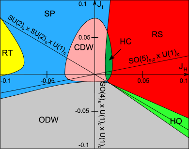
Figure 2: Low-energy phase diagram of the generalized Hund model at half-filling for $U=-0.005t$ ($t=1$). (SP=Spin Peierls, CDW=Charge density wave, ODW=Orbital density wave, RS=Rung Singlet, HC=Haldane Charge, HO=Haldane Orbital, RT=Rung Triplet). At the intersection of the highly symmetric lines lie points with even larger symmetry (see Table I).

The duality approach that we used to obtain the phase diagram allows for an easy characterization of the quantum phase transitions. Those transitions are located on the self-dual lines, where the coupling constants that change their sign when going from one phase to the other vanish. Fig. (3) summarizes all the phase transitions that occur in the phase diagram of the generalized Hund model.

Figure 3: Quantum phase transitions that can occur in the generalized Hund model. The letter next to the arrows indicates which degrees of freedom are critical: c=charge, s=spin, o=orbital.

We now present the zero-temperature phase diagram of several interesting highly symmetric models with two independent coupling constants that we have introduced in Section II.

III.3.2 Phase diagram of the SO(5) fermionic cold atoms model

Let us start with the spin-$\frac{3}{2}$ cold fermionic atoms model (6) which is obtained from the generalized Hund model (1) by the fine tuning $J_{H}=4J_{t}$. In the continuum limit, the coupling constants are naturally parametrized by the singlet and quintet pairing $U_{0}$ and $U_{2}$: $g_{1}=g_{2}=g_{5}=-U_{0}-U_{2},g_{3}=g_{4}=U_{0}-3U_{2},g_{6}=U_{0}+5U_{2},g_{7}=g_{8}=2U_{2},g_{9}=2U_{0}$. The effective Majorana model (19), describing the physical properties of the spin-$\frac{3}{2}$ cold fermions model, depends on five independent coupling constants. The resulting phase diagram, as obtained from the one-loop RG calculation, is presented in Fig. 4.

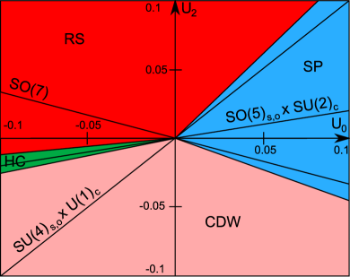
Figure 4: Phase diagram of the spin-$\frac{3}{2}$ cold fermions model at half-filling ($t=1$).

III.3.3 SO(5) SZH model

As mentioned in the introduction, there is a second SO(5)-symmetric model embedded in the generalized Hund model (1): the SZH model (8). In the latter model, obtained from (1) when $J_{H}=8U$, the SO(5) symmetry unifies charge and spin degrees of freedom szh . The coupling constants of the Majorana model (19) for the SZH model (8) read as follows:

$$g_{1,6,7} = a_{0}\left(U_{\textrm{SZH}}+2V_{\textrm{SZH}}\right)$$

$$g_{2,8} = a_{0}U_{\textrm{SZH}}$$

$$g_{3,9} = -a_{0}\left(3U_{\textrm{SZH}}+2V_{\textrm{SZH}}\right)$$

$$g_{4} = -a_{0}\left(3U_{\textrm{SZH}}+4V_{\textrm{SZH}}\right)$$

$$g_{5} = a_{0}\left(U_{\textrm{SZH}}-2V_{\textrm{SZH}}\right).$$ (52)

We obtain the phase diagram shown in Fig. (5).

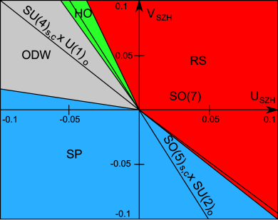
Figure 5: Phase diagram of the SZH model (8) with the fine-tuning $J_{\textrm{SZH}}=4(U_{\textrm{SZH}}+V_{\textrm{SZH}})$ at half-filling ($t=1$).

The phases are very similar to the one in the spin-$\frac{3}{2}$ cold fermions model with the substitution: CDW $\to$ ODW and HC $\to$ HO.

III.3.4 Phase diagram of SO(4) models

We now turn to models which display an extended SO(4) symmetry. In Section II, we found two different SO(4) models with two independent coupling constants, i.e., one fine-tuning with respect to the original generalized Hund model (1). When $J_{H}=0$, the lattice model (5) enjoys a U(1)_c $\times$ U(1)_o $\times$ SO(4)_s continuous symmetry. The phase diagram of this model can be determined by the low-energy approach from the identification of the coupling constants of model (19):

$$g_{1}=g_{3}=-a_{0}\left(U+\frac{J_{t}}{2}\right)$$

$$g_{2}=g_{4}=-a_{0}\left(U-\frac{J_{t}}{2}\right)$$

$$g_{5}=-a_{0}\left(U-\frac{3J_{t}}{2}\right)$$

$$g_{6}=a_{0}\left(3U-\frac{J_{t}}{2}\right)$$

$$g_{7}=g_{9}=-g_{2}=-g_{4}$$

$$g_{8}=-g_{1}=-g_{3}.$$ (53)

The resulting phase diagram is presented in Fig. 6. It contains an interesting line $J_{t}=2U$ with enlarged SO(4)_c,o $\times$ SO(4)_s symmetry (see Section II). It is straightforward to see that along this line for $U<0$, where the transition between the CDW and ODW appears, the spin degrees of freedom are gapped while the charge and orbital degrees of freedom are critical. Hence, the quantum phase transition is described by a SO(4)₁ CFT with central charge $c=2$.

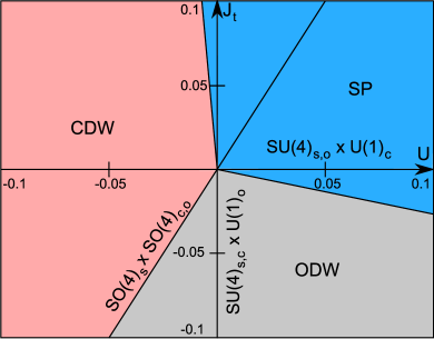
Figure 6: Phase diagram of the SO(4) model (5) with $J_{H}=0$ ($t=1$) at half-filling. The continuous symmetry group is U(1)_c $\times$ U(1)_o $\times$ SO(4)_s.

The second model is defined for $J_{t}=2U$ (see Table I) with SO(4)_c,o $\times$ SU(2)_s continuous symmetry. Here, the SO(4) symmetry unifies the charge and orbital degrees of freedom. The coupling constants of the continuum limit of this model are given by

$$g_{1}=-a_{0}\left(2U-\frac{J_{H}}{2}\right)$$

$$g_{2}=g_{7}=a_{0}\frac{J_{H}}{4}$$

$$g_{3}=-a_{0}\left(2U+\frac{J_{H}}{2}\right)$$

$$g_{4}=g_{9}=-a_{0}\frac{3J_{H}}{4}$$

$$g_{5}=g_{6}=g_{8}=2a_{0}U,$$ (54)

from which we deduce the phase diagram of Fig. 7.

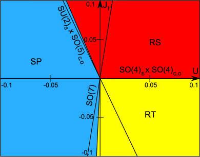
Figure 7: Phase diagram of the half-filled SO(4) model with $J_{t}=2U$ ($t=1$) which unifies charge and orbital degrees of freedom.

The quantum phase transition between RS and RT phases for $J_{H}=0$ and $U>0$ is now governed by the spin degrees freedom and the SO(4)₁ CFT.

III.3.5 Phase diagram of spin-orbital (charge) models

The generalized Hund model (1) reduces to the spin-orbital model when $J_{t}=-3J_{H}/4$ with a U(1)_c $\times$ SU(2)_o $\times$ SU(2)_s symmetry which has been studied in the context of orbital degeneracy yamashita ; khomskii ; mila ; aza4spin ; itoi00 . The coupling constants of the continuum limit of this model read as follows:

$$g_{1}=-a_{0}\left(U-\frac{7J_{H}}{8}\right)$$

$$g_{2}=g_{3}=-a_{0}\left(U+\frac{J_{H}}{8}\right)$$

$$g_{4}=g_{5}=-a_{0}\left(U+\frac{9J_{H}}{8}\right)$$

$$g_{6}=a_{0}\left(3U+\frac{3J_{H}}{8}\right)$$

$$g_{7}=a_{0}\left(U+\frac{5J_{H}}{8}\right)$$

$$g_{8}=g_{9}=a_{0}\left(U-\frac{3J_{H}}{8}\right).$$ (55)

The phase diagram of the spin-orbital model is presented in Fig. 8. In particular, it includes two non-degenerate Mott-insulating phases: HO and RT phases.

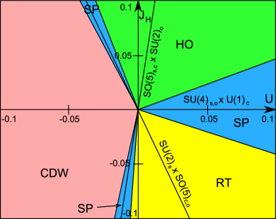
Figure 8: Phase diagram of the spin-orbital model at half-filling with $J_{t}=-3J_{H}/4$ ($t=1$).

Finally, we consider the related spin-charge model which is defined for the fine-tuning $J_{H}=-8U/3$ with U(1)_o $\times$ SU(2)_c $\times$ SU(2)_s continuous symmetry at half-filling. The resulting model is similar to the spin-orbital model where now spin and charge are put on the same footing. We find the following continuum limit for the spin-charge model:

$$g_{1}=-a_{0}\left(\frac{7U}{3}+\frac{J_{t}}{2}\right)$$

$$g_{2}=-a_{0}\left(\frac{5U}{3}-\frac{J_{t}}{2}\right)$$

$$g_{3}=g_{7}=a_{0}\left(\frac{U}{3}-\frac{J_{t}}{2}\right)$$

$$g_{4}=g_{8}=a_{0}\left(U+\frac{J_{t}}{2}\right)$$

$$g_{5}=-a_{0}\left(U-\frac{3J_{t}}{2}\right)$$

$$g_{6}=g_{9}=a_{0}\left(3U-\frac{J_{t}}{2}\right).$$ (56)

Its phase diagram is depicted in Fig. 9. Here, two non-degenerate Mott insulating phases appear: the HC and RT phases.

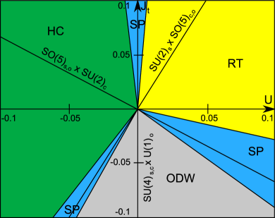
Figure 9: Phase diagram of the spin-charge model at half-filling with $J_{H}=-8U/3$ ($t=1$). The symmetry is: $SU(2)_{s}\times SU(2)_{c}\times U(1)_{o}$.

III.4 Effect of an interchain hopping term

Let us now consider the generalized Hund model (1) to which we add an interchain hopping term:

$$\mathcal{H}_{\bot}=-t_{\bot}\sum_{i,\,\sigma}\left(c^{\dagger}_{1\sigma,\,i}c^{\phantom{{\dagger}}}_{2\sigma,\,i}+\mbox{h.c.}\right).$$ (57)

This problem has been previously studied and its phases are known Linso8 ; furusaki ; wu04 . We will show that all those phases (there are eight of them) can be connected one-by-one (by a non-trivial duality) to the phases of the generalized Hund model (1). Our approach will use a weak coupling analysis, and our conclusion relies on the existence of a hidden orbital symmetry emerging at low-energy. In Appendix C, we show that this approach is also valid in the strong coupling regime, close to the orbital line $J_{t}=-3J_{H}/4$.

In the presence of interchain hopping, the non-interacting part of the Hamiltonian cannot be readily diagonalized. We need to do a change of basis and introduce bonding and antibonding operators:

$$d^{\phantom{{\dagger}}}_{j\sigma}=\frac{1}{\sqrt{2}}\left(c^{\phantom{{\dagger}}}_{1\sigma}+(-1)^{j}c^{\phantom{{\dagger}}}_{2\sigma}\right).$$ (58)

Using this basis, the kinetic part can be diagonalized in momentum space; there are now two decoupled bands (bonding and antibonding bands) and two Fermi points (provided $t_{\bot}<2t$) $k_{F_{1}}$ and $k_{F_{2}}$ such that, at half-filling, $k_{F_{1}}+k_{F_{2}}=\pi/a_{0}$. One could proceed by linearizing around the four Fermi points, by introducing continuous bonding and antibonding fermionic fields $R_{a\sigma}(x)$ and $L_{a\sigma}(x)$ (with $a=1,2$, $\sigma=\uparrow,\downarrow$) by bosonizing, refermionizing, and expanding the interactions in this basis. Instead, we will follow an approach that is based on the (continuous) symmetry content of the theory, by showing that the symmetry of the low energy, continuous theory is essentially the same for $t_{\perp}\neq 0$ as for $t_{\perp}=0$.

This is not obvious: naively, the interchain hopping term breaks the U(1)_o orbital symmetry and the analysis of the preceding sections breaks down. However, as noticed before Linso8 ; wu04 , at low energy another U(1) symmetry emerges in the orbital sector. To see this, let us consider the difference $\delta=k_{F1}-k_{F2}=2\arcsin(t_{\perp}/2t)$. It is a continuous function of $t_{\perp}$, and provided $\delta$ is not commensurate to $\pi$, in the continuum limit and at weak coupling, one can safely ignore umklapp terms that oscillate at wave-vector that are integer multiples of $\delta$. Retaining only marginal, four-fermions interactions of the form $\prod_{i=1}^{4}\Psi^{(i)}_{a_{i}\sigma_{i}}$, with $\Psi^{(i)}=R,L$, one sees that in order for this term to be non-oscillating and to give a contribution to the interacting part of the continuous theory, it has to conserve separately the quantities $\rho_{+}=N_{1R}+N_{2L}$ and $\rho_{-}=N_{1L}+N_{2R}$, where $N_{aL}=\sum_{\sigma}\int dx\,L^{\dagger}_{a\sigma}L_{a\sigma}$ and $N_{aR}=\sum_{\sigma}\int dx\,R^{\dagger}_{a\sigma}R_{a\sigma}$ are the total number of left (right) fermions in each of the bonding and antibonding bands. It results that the difference $\rho_{+}-\rho_{-}=(N_{1R}-N_{2R})-(N_{1L}-N_{2L})$ is conserved: this is nothing but (twice) the total orbital current in the bonding/antibonding basis along direction $z$. This quantity generates a U(1) orbital symmetry $\widetilde{\mbox{U(1)}}_{o}$. One thus concludes that the low-energy continuous theory has a symmetry U(1)${}_{c}\times$SU(2)${}_{s}\times\widetilde{\mbox{U(1)}}_{o}\times Z_{2}$, the same has in the $t_{\perp}=0$ case.

The total orbital current $\rho_{+}-\rho_{-}$ can be mapped onto the total orbital charge (all other conserved quantities, i.e., the electric charge and the SU(2)_s spin generators, being unaffected) by the duality $\Omega_{\perp}$ that leaves all Majorana fermions $(\xi^{a})_{a\neq 5}$ invariant, but changes $\xi^{5}_{L}$ to $-\xi^{5}_{L}$. The duality $\Omega_{\perp}$ is highly non-local. A little algebra shows that it has the following action on the bonding and antibonding modes ($a=1,2$):

$$L^{\phantom{{\dagger}}}_{a\,\uparrow}\to L^{\dagger}_{a\,\downarrow},\quad L^{\phantom{{\dagger}}}_{a\,\downarrow}\to-L^{\dagger}_{a\,\uparrow}.$$ (59)

Table 2: Pattern of the bosonic fields pinning for $t_{\bot}=0$ and $t_{\bot}\neq 0$.

Phase	$\langle\Phi_{c}\rangle$	$\langle\Phi_{s}\rangle$	$\langle\Phi_{f}\rangle$	$\langle\Phi_{sf}\rangle$	$\langle\Theta_{sf}\rangle$	Phase	$\langle\Phi_{c}\rangle$	$\langle\Phi_{s}\rangle$	$\langle\Theta_{f}\rangle$	$\langle\Phi_{sf}\rangle$	$\langle\Theta_{sf}\rangle$
SP	$0$	0	0	0	-	S-Mott	$0$	0	$\sqrt{\pi}/2$	0	-
CDW	$\sqrt{\pi}/2$	0	0	0	-	S’-Mott	$\sqrt{\pi}/2$	0	$\sqrt{\pi}/2$	0	-
ODW	$0$	0	$\sqrt{\pi}/2$	0	-	D-Mott	0	0	0	0	-
SPπ	$\sqrt{\pi}/2$	0	$\sqrt{\pi}/2$	0	-	D’-Mott	$\sqrt{\pi}/2$	0	0	0	-
RS	0	0	0	-	0	CDWπ	0	0	$\sqrt{\pi}/2$	-	0
HC	$\sqrt{\pi}/2$	0	0	-	0	PDW	$\sqrt{\pi}/2$	0	$\sqrt{\pi}/2$	-	0
HO	0	0	$\sqrt{\pi}/2$	-	0	SF	0	0	0	-	0
RT	0	$\sqrt{\pi}/2$	0	-	$\sqrt{\pi}/2$	FDW	0	$\sqrt{\pi}/2$	$\sqrt{\pi}/2$	-	$\sqrt{\pi}/2$

With those elements at hand, the general form of the low-energy Hamiltonian can thus be readily deduced from (19) by performing the replacement $\xi^{5}_{L}\to-\xi^{5}_{L}$. While this approach tells nothing about the (bare) value of the coupling constants $g_{a}$, it tells us that the structure of the RG equations (51) is the same, and is thus sufficient to $(i)$ enumerate the phases of the model and $(ii)$ relate each of those phases to the phases of the generalized Hund model (1).

From the preceding sections ($t_{\bot}=0$), we deduce that there are eight possible insulating phases. The effect of the duality $\Omega_{\bot}$ is to transform the bosonic field $\Phi_{f}$ into its dual with a shift of $\sqrt{\pi}/2$: $\Phi_{f}\xrightarrow{\;\;\Omega_{\bot}}\Theta_{f}+\sqrt{\pi}/2$. We then obtain the pinnings of the bosonic fields from those found for $t_{\bot}=0$ via the duality $\Omega_{\bot}$; they are summarized in Table 2. In the language of Ref. boulat, , $\Omega_{\bot}$ is an outer duality (it affects only one Majorana fermion, or equivalently, it maps a bosonic field onto its dual): it results that it maps degenerate phases onto non-degenerate ones and vice-versa.

The pinnings of Table 2 allow us to identify each phase with one of the already known phases of the generalized two-leg Hubbard ladder Linso8 ; furusaki ; wu04 . The SP phase becomes an S-Mott phase with order parameter:

$${\cal O}_{\text{S-Mott}}=\sum_{i,l}c_{l\uparrow,i}c_{l\downarrow,i}.$$ (60)

The CDW phase becomes the D-Mott phase, which is the same phase as RS, and is characterized by the order parameter:

$${\cal O}_{\text{D-Mott}}=\sum_{i}c_{1\uparrow,i}c_{2\downarrow,i}-c_{2\uparrow,i}c_{1\downarrow,i}.$$ (61)

The ODW (respectively SP_π) phase give an S’-Mott (respectively D’-Mott) state which differs from the S-Mott (respectively D-Mott) only in the pinning of the charge bosonic field $\Phi_{c}$ (see Table 2) furusaki . Such order parameters have the slowest decaying correlation function when the system is doped. The non-degenerate RS phase will become the two-fold degenerate CDW_π phase with an inter-leg phase difference comment :

$${\cal O}_{\text{CDW-}\pi}=\sum_{i,l\sigma}(-1)^{i}(-1)^{l+1}c^{\dagger}_{l\sigma,i}c^{\phantom{{\dagger}}}_{l\sigma,i}.$$ (62)

The HC phase becomes a p-density wave (PDW) phase which is described by the condensation of the order parameter comment2 :

$${\cal O}_{\text{PDW}}=\sum_{i,l\sigma}(-1)^{i}(-1)^{l+1}\left(c^{{\dagger}}_{l\sigma,i}c^{\phantom{{\dagger}}}_{l\sigma,i+1}+\mbox{h.c.}\right).$$ (63)

The HO phase gives a staggered flux (SF) phase (or a d-density wave phase) whose ground states display currents circulating around a plaquette, with order parameter:

$${\cal O}_{\text{SF}} = i\sum_{i,\sigma}(c^{\dagger}_{1\sigma,i}c^{\phantom{{\dagger}}}_{2\sigma,i}+c^{{\dagger}}_{2\sigma,i}c^{\phantom{{\dagger}}}_{2\sigma,i+1}$$ (64)

$$+ c^{{\dagger}}_{2\sigma,i+1}c^{\phantom{{\dagger}}}_{1\sigma,i+1}+c^{{\dagger}}_{1\sigma,i+1}c^{\phantom{{\dagger}}}_{1\sigma,i}-\mbox{h.c.}).$$

This phase spontaneously breaks time-reversal symmetry. Finally, the RT phase will become a f-density wave (FDW). This phase consists in currents flowing along the diagonals of plaquettes:

$${\cal O}_{\text{FDW}} = i\sum_{i,\sigma}(c^{\dagger}_{2\sigma,i+1}c^{\phantom{{\dagger}}}_{1\sigma,i}-c^{{\dagger}}_{1\sigma,i}c^{\phantom{{\dagger}}}_{2\sigma,i+1}$$ (65)

$$+ c^{{\dagger}}_{1\sigma,i+1}c^{\phantom{{\dagger}}}_{2\sigma,i}-c^{{\dagger}}_{2\sigma,i}c^{\phantom{{\dagger}}}_{1\sigma,i+1}).$$

It also breaks time-reversal symmetry.

As already emphasized, the emergent duality symmetry $\Omega_{\bot}$ provides only a correspondence between the set of phases with $t_{\perp}=0$ with those of $t_{\perp}\neq 0$. By no means, it maps a given model defined by $(t_{\perp}=0,U,J_{H},J_{t})$ onto the model $(t_{\perp}\neq 0,U,J_{H},J_{t})$. In this respect, it is necessary to use the one-loop RG calculation to map out the phase diagram of the generalized Hund chain with a transverse hopping. Using Eq. (51) and the initial conditions for that model

$$g_{1}=a_{0}\left(-U+\frac{J_{H}}{2}-\frac{J_{t}}{2}\right)$$

$$g_{2}=a_{0}\left(-\frac{3J_{H}}{8}-\frac{J_{t}}{2}\right)$$

$$g_{3}=a_{0}\left(-U+\frac{J_{H}}{4}+\frac{J_{t}}{2}\right)$$

$$g_{4}=g_{2}$$

$$g_{5}=a_{0}\left(U+\frac{3J_{H}}{4}-\frac{J_{t}}{2}\right)$$

$$g_{6}=a_{0}\left(3U-\frac{J_{t}}{2}\right)$$

$$g_{7}=a_{0}\left(U+\frac{J_{H}}{4}-\frac{J_{t}}{2}\right)$$

$$g_{8}=g_{2}$$

$$g_{9}=a_{0}\left(U+\frac{J_{t}}{2}\right),$$ (66)

we find the presence of the eight insulating phases. Figure 10 presents a section of the phase diagram for $U=-0.005t$ where the eight phases are revealed. Interestingly enough, the generalized Hund chain model with a transverse hopping turns out to be the minimal model for two-leg electronic ladder models which contains the eight insulating phases found within the low-energy approach furusaki ; wu04 . In particular, one does not need to add further interactions (first neighbors density interactions for instance) contrarily to Refs. furusaki, ; wu04, .

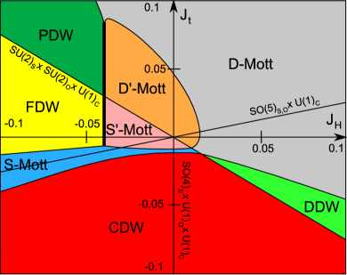
Figure 10: The eight fully gapped phases of the generalized Hund chain with a transverse hopping at half-filling ($U=-0.005t$).

IV DMRG calculations

We now carry out numerical calculations using DMRG in order to investigate the various phase diagrams. For simplicity, we will restrict ourselves to the $t_{\perp}=0$ case for which we can use a purely one-dimensional implementation of the model. Moreover, for a system of finite size $L$, we can fix the total number of particles $N=2Q_{c}=2\sum_{i}n_{c,i}=2L$, the $z$-component of the total spin $S^{z}=\sum_{i}n_{s,i}$ as well as the $z$-component of the total orbital operator $T^{z}=\sum_{i}n_{f,i}$ (see Eq. (39)), so that the states are labeled by the triplet $(Q_{c},S^{z},T^{z})$. Typically, we keep up to 1600 states, which allow to have an error below $10^{-6}$, and we use open boundary conditions (OBC).

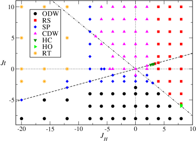
Figure 11: Numerical phase diagram of the generalized Hund model at half-filling for $U=-t$. Notations are the same as in Fig. 2.

As it has been revealed by the low-energy approach, there are eight possible insulating phases, that are related by duality transformations. In order to characterize them, we can either compute local quantities (bond kinetic energy, local density, …) to identify states that break a given symmetry, or investigate the presence or absence of various edge states to detect non-degenerate Mott phases. Thus, the three possible Haldane phases that have been predicted (RT, HC, and HO) can be characterized by looking for the presence of edge states with quantum numbers $(Q_{c},S_{z},T_{z})$ respectively equal to $(L,1,0)$, $(L+1,0,0)$ and $(L,0,1)$ (see details in Appendix B).

From these measurements, we can draw various cuts of the phase diagram in the $(U,J_{H},J_{t})$ parameter space. In Fig. 11, we present our data for fixed $U=-t$. Seven (out of eight) insulating phases are found and the overall topology nicely agrees with the low-energy predictions shown in Fig. 2, although those were obtained with a much weaker interaction $U=-0.005t$. As another example, we consider a highly symmetric case, namely the SZH model (see Section  III.3.3), which corresponds to the case $J_{H}=8U$. We recall that the low-energy phase diagram of this model is shown in Fig. 5. The numerical phase diagram (Fig. 12) is in excellent agreement not only for the overall topology but also for the location of the phase boundaries.

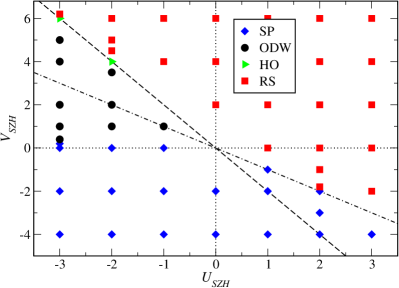
Figure 12: Numerical phase diagram of the SZH SO(5) model with the fine-tuning $J_{SZH}=4(U_{SZH}+V_{SZH})$ at half-filling. Notations are the same as in Fig. 5. Dashed lines indicate models with higher symmetry (see Table 1).

Finally, we also did simulations for the spin-orbital model obtained by fixing $J_{t}=-3J_{H}/4$. In that case as well, we observe that the low-energy predictions (see Fig. 8) and our numerical data (see Fig. 13) coincide very well.

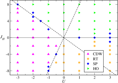
Figure 13: Numerical phase diagram of the spin-orbital model ($J_{t}=-3J_{H}/4$) at half-filling. Notations are the same as in Fig. 8. Dashed lines indicate models with higher symmetry (see Table 1).

In brief, for all the cases we considered when $t_{\perp}=0$, we obtain an excellent agreement between the low-energy predictions (obtained for very weak couplings) and the numerical phase diagram (obtained at moderate couplings). This is an important result of our paper.

The case of a transverse hopping $t_{\perp}\neq 0$ is much more difficult to analyze with respect to the low-energy approach. As discussed in Section III D, in the latter approach, there is an emergent $\widetilde{\mbox{U(1)}}$ symmetry in the orbital space which is not present on the lattice. It means that we need to consider long-size systems in the DMRG calculations in order to compare with the low-energy predictions. A second difficulty arises with respect to the numerical discrimination between the S-Mott (respectively D-Mott) phase and the S’-Mott (respectively D’-Mott) phase. A numerical analysis of relevant string-order parameters is clearly called for to distinguish them. To the best of our knowledge, we are not aware of any numerical study which reports the existence of the (S,D)’-Mott phases in generalized two-leg electronic ladders. We plan to investigate elsewhere the numerical phase diagram of the generalized Hund model with a transverse hopping.

V Concluding Remarks

In summary, we have investigated the phase diagram of the generalized Hund model (1) with global symmetry group H $=$ U(1)_c $\times$ SU(2)_s $\times$ U(1)_o $\times$ Z₂ at half-filling by means of complementary low-energy and DMRG techniques. The interest of this model is manifold. First, it covers and unifies several highly symmetric lattice models: the SO(5)-symmetric model describing spin-$\frac{3}{2}$ cold fermions; another (different) SO(5)-symmetric model introduced by Scalapino, Zhang and Hanke that unifies antiferromagnetism and d-wave superconductivity; and two SU(2)$\times$SU(2)-symmetric spin-orbital models. While its orbital U(1) symmetry can seem a little odd from the point of view of applications to the description of Hubbard two-leg ladders, we show that at weak-coupling, it shares the same continuous low-energy effective theory with the well known Hubbard two-leg ladder with interchain hopping. Third, it is directly relevant to the description of Ytterbium 171 loaded into an optical 1D trap. We are able to treat on an equal footing all the phases appearing in those models coming from different contexts. The rich phase diagram of the generalized Hund model has to be contrasted with the minimal character and simplicity of this model, which only depends on three microscopic couplings.

We briefly recall our main results: by means of a duality approach, we predict that the phase diagram for half-filled four-component fermions with global symmetry H $=$ U(1)_c $\times$ SU(2)_s $\times$ U(1)_o $\times$ Z₂ consists in eight Mott-insulating phases. These phases fall into two different classes. A first class consists of two-fold degenerate fully gapped density phases which spontaneously break a discrete symmetry present on the lattice. The second class comprises four non-degenerate Mott-insulating phases which are characterized by non-local string order parameters: RS, RT, HC, and HO phases. A one-loop RG calculation for model (1) reveals the existence of seven phases out of the eight ones consistent with the duality approach. The missing phase, which can be found by adding further nearest-neighbor interactions, is an alternating bond ordered phase (SP_π). These results have been confirmed numerically by means of a DMRG approach for moderate couplings. In this respect, we found an excellent agreement between the two complementary approaches.

Finally, we have connected our low-energy results to the eight previously known insulating phases found in generalized two-leg ladders with a transverse hopping $t_{\perp}$ term. When $t_{\perp}\neq 0$, the U(1) orbital symmetry is lost on the lattice but becomes an emergent symmetry at low-energy. The duality approach with global symmetry group H can then still be applied in the presence of a interchain hopping $t_{\perp}$ term. In this respect, we discovered a non-local duality which maps the eight Mott-insulating phases for $t_{\perp}=0$ onto the eight phases previously known for $t_{\perp}\neq 0$. The one-loop RG approach to the generalized Hund model with interchain hopping predicts the stabilization of the eight Mott-insulating phases. The latter model is thus the minimal model for two-leg electronic ladders which displays the eight Mott-insulating phases at weak coupling. We also discuss the fate of this emergent U(1) orbital symmetry when going from the weak-coupling to the strong coupling regime. We show that the weak- and strong-coupling phases coincide in the vicinity of the orbital symmetric line, but our analysis suggests a breakdown of this picture away from this special line.

We hope that future experiments on ¹⁷¹Yb or alkaline-earth cold fermions atoms loaded into a 1D optical lattice will reveal some of the exotic insulating phases found in our study.

Appendix A Continuum Limit

In this Appendix, we present the technical details of the continuum limit of the generalized Hund model (1). The starting point of the low-energy approach is the linearization around the Fermi points $\pm k_{F}$ of the dispersion relation for non-interacting fermions. Four left and right moving Dirac fermions $L_{l\sigma},R_{l\sigma}$ ($l=1,2$ and $\sigma=\uparrow,\downarrow$) are then introduced to describe the lattice fermions $c_{l\sigma,i}$ in the continuum limit (see Eq. (16)).

The next step of the approach is the introduction of four chiral bosonic fields $\Phi_{l\sigma R,L}$ through the Abelian bosonization of Dirac fermions bookboso ; giamarchi :

$$R_{\,l\sigma} = \frac{\kappa_{l\sigma}}{\sqrt{2\pi a_{0}}}\exp{\left(i\sqrt{4\pi}\Phi_{l\sigma R}\right)}$$

$$L_{l\sigma} = \frac{\kappa_{l\sigma}}{\sqrt{2\pi a_{0}}}\exp{\left(-i\sqrt{4\pi}\Phi_{l\sigma L}\right)},$$ (67)

where the bosonic fields satisfy the following commutation relation:

$$\left[\Phi_{l\sigma R},\Phi_{l^{\prime}\sigma^{\prime}L}\right]=\frac{i}{4}\delta_{ll^{\prime}}\delta_{\sigma\sigma^{\prime}}.$$ (68)

The presence of the Klein factors $\kappa_{l\sigma}$ ensures the correct anticommutation of the fermionic operators. The Klein factors satisfy the anticommutation rule $\{\kappa_{l\sigma},\kappa_{l^{\prime}\sigma^{\prime}}\}=2\delta_{ll^{\prime}}\delta_{\sigma\sigma^{\prime}}$ and they are constrained so that $\Gamma^{2}=1$, with $\Gamma=\kappa_{1\uparrow}\kappa_{1\downarrow}\kappa_{2\uparrow}\kappa_{2\downarrow}$. Hereafter, we will work within the $\Gamma=1$ sector. It will be convenient to work with a pair of dual non-chiral bosonic fields: $\Phi_{l\sigma}=\Phi_{l\sigma L}+\Phi_{l\sigma R}$ and $\Theta_{l\sigma}=\Phi_{l\sigma L}-\Phi_{l\sigma R}$. Last, let us introduce a SU(4) basis that will allow us to separate charge and non-Abelian (spin) degrees of freedom:

$$\Phi_{1\uparrow}=\frac{1}{2}(\Phi_{c}+\Phi_{s}+\Phi_{f}+\Phi_{sf})$$

$$\Phi_{1\downarrow}=\frac{1}{2}(\Phi_{c}-\Phi_{s}+\Phi_{f}-\Phi_{sf})$$

$$\Phi_{2\uparrow}=\frac{1}{2}(\Phi_{c}+\Phi_{s}-\Phi_{f}-\Phi_{sf})$$

$$\Phi_{2\downarrow}=\frac{1}{2}(\Phi_{c}-\Phi_{s}-\Phi_{f}+\Phi_{sf}).$$ (69)

In sharp contrast with incommensurate fillings, there is no spin charge separation at half-filling. Indeed, in this special case, chiral umklapp processes couple those degrees of freedom. Consequently, the resulting low-energy Hamiltonian corresponding to model (1) takes the form: $\mathcal{H}=\mathcal{H}_{c}+\mathcal{H}_{s}+\mathcal{H}_{\textrm{umklapp}}$.

The charge degrees of freedom are described by:

$$\mathcal{H}_{c}=\frac{v_{F}}{2}\left[(\partial_{x}\Phi_{c})^{2}+(\partial_{x}\Theta_{c})^{2}\right]+\Delta v_{c}\,(\partial_{x}\Phi_{c})^{2},$$ (70)

where $v_{F}=a_{0}t$ is the Fermi velocity.

The part of the bosonized Hamiltonian corresponding to the non-abelian degrees of freedom is:

$$\mathcal{H}_{s} = \frac{v_{F}}{2}\sum_{a=s,f,sf}\left[(\partial_{x}\Phi_{a})^{2}+(\partial_{x}\Theta_{a})^{2}\right]$$ (71)

$$+ \sum_{a=s,f,sf}\Delta v_{a}\,(\partial_{x}\Phi_{a})^{2}$$

$$+ A_{1}\left(C_{sfR}^{\sqrt{16\pi}}+C_{sfL}^{\sqrt{16\pi}}\right)$$

$$+ A_{2}\left(C_{s}^{\sqrt{4\pi}}+C_{f}^{\sqrt{4\pi}}\right)\tilde{C}_{sf}^{\sqrt{4\pi}}+A_{3}\,C_{s}^{\sqrt{4\pi}}C_{f}^{\sqrt{4\pi}}$$

$$+ A_{4}\,C_{s}^{\sqrt{4\pi}}C_{sf}^{\sqrt{4\pi}}+A_{5}\,C_{f}^{\sqrt{4\pi}}C_{sf}^{\sqrt{4\pi}},$$

where we used the compact notation: $C_{a}^{\beta}=\cos{(\beta\Phi_{a})}$, and $\tilde{C}_{a}^{\beta}=\cos{(\beta\Theta_{a})}$. The bare parameters are:

$$\Delta v_{c}=\frac{a_{0}}{\pi}\left(\frac{3U}{2}-\frac{J_{t}}{4}\right)$$

$$\Delta v_{s}=-\frac{a_{0}}{\pi}\left(\frac{U}{2}-\frac{J_{H}}{4}+\frac{J_{t}}{4}\right)$$

$$\Delta v_{f}=-\frac{a_{0}}{\pi}\left(\frac{U}{2}-\frac{3J_{t}}{4}\right)$$

$$\Delta v_{sf}=-\frac{a_{0}}{\pi}\left(\frac{U}{2}+\frac{J_{H}}{4}+\frac{J_{t}}{4}\right)$$

$$A_{1}=-\frac{J_{H}a_{0}}{4\pi^{2}}$$

$$A_{2}=-\frac{J_{H}a_{0}}{2\pi^{2}}$$

$$A_{3}=\frac{a_{0}}{\pi^{2}}\left(U-\frac{J_{H}}{4}-\frac{J_{t}}{2}\right)$$

$$A_{4}=\frac{a_{0}}{\pi^{2}}\left(U+\frac{J_{t}}{2}\right)$$

$$A_{5}=\frac{a_{0}}{\pi^{2}}\left(U+\frac{J_{H}}{4}-\frac{J_{t}}{2}\right).$$ (72)

Finally, the umklapp part of the Hamiltonian reads:

$$\mathcal{H}_{\textrm{umklapp}} = A_{6}\,C_{c}^{\sqrt{4\pi}}C_{s}^{\sqrt{4\pi}}+A_{7}\,C_{c}^{\sqrt{4\pi}}C_{f}^{\sqrt{4\pi}}$$ (73)

$$+ A_{8}\,C_{c}^{\sqrt{4\pi}}C_{sf}^{\sqrt{4\pi}}+A_{9}\,C_{c}^{\sqrt{4\pi}}\tilde{C}_{sf}^{\sqrt{4\pi}},$$

with

$$A_{6}=\frac{a_{0}}{\pi^{2}}\left(-U-\frac{J_{H}}{4}+\frac{J_{t}}{2}\right)$$

$$A_{7}=\frac{a_{0}}{\pi^{2}}\left(-U-\frac{J_{t}}{2}\right)$$

$$A_{8}=\frac{a_{0}}{\pi^{2}}\left(-U+\frac{J_{H}}{4}+\frac{J_{t}}{2}\right)$$

$$A_{9}=A_{2}=-\frac{J_{H}a_{0}}{2\pi^{2}}\,.$$ (74)

In the end, a refermionization procedure will allow us to make the exact U(1)_c $\times$ SU(2)_s $\times$ U(1)_o $\times$ Z₂ continuous symmetry explicit in the effective Hamiltonian. For this purpose, we introduce eight left and right moving Majorana fermions through:

$$\xi_{L}^{2}+i\xi_{L}^{1}=\frac{\eta_{1}}{\sqrt{\pi a_{0}}}\exp{(-i\sqrt{4\pi}\Phi_{sL})}$$

$$\xi_{R}^{2}+i\xi_{R}^{1}=\frac{\eta_{1}}{\sqrt{\pi a_{0}}}\exp{(i\sqrt{4\pi}\Phi_{sR})}$$

$$\xi_{L}^{4}-i\xi_{L}^{5}=\frac{\eta_{2}}{\sqrt{\pi a_{0}}}\exp{(-i\sqrt{4\pi}\Phi_{fL})}$$

$$\xi_{R}^{4}-i\xi_{R}^{5}=\frac{\eta_{2}}{\sqrt{\pi a_{0}}}\exp{(i\sqrt{4\pi}\Phi_{fR})}$$

$$\xi_{L}^{6}+i\xi_{L}^{3}=\frac{\eta_{3}}{\sqrt{\pi a_{0}}}\exp{(-i\sqrt{4\pi}\Phi_{sfL})}$$

$$\xi_{R}^{6}+i\xi_{R}^{3}=\frac{\eta_{3}}{\sqrt{\pi a_{0}}}\exp{(i\sqrt{4\pi}\Phi_{sfR})}$$

$$\xi_{L}^{8}+i\xi_{L}^{7}=\frac{\eta_{4}}{\sqrt{\pi a_{0}}}\exp{(-i\sqrt{4\pi}\Phi_{cL})}$$

$$\xi_{R}^{8}+i\xi_{R}^{7}=\frac{\eta_{4}}{\sqrt{\pi a_{0}}}\exp{(i\sqrt{4\pi}\Phi_{cR})},$$ (75)

where $\eta_{1,2,3,4}$ are again Klein factors which ensure the adequate anticommutation rules for the fermions. Using this correspondence rules, equations (70, 71,73) can be expressed in terms of these eight Majorana fermions. We thus finally obtain the low-energy effective theory for the generalized Hund model (1) at half-filling:

$$\mathcal{H} = -\frac{iv_{c}}{2}\sum_{a=7}^{8}(\xi_{R}^{a}\partial_{x}\xi_{R}^{a}-\xi_{L}^{a}\partial_{x}\xi_{L}^{a})$$ (76)

$$- \frac{iv_{s}}{2}\sum_{a=1}^{3}(\xi_{R}^{a}\partial_{x}\xi_{R}^{a}-\xi_{L}^{a}\partial_{x}\xi_{L}^{a})$$

$$- \frac{iv_{t}}{2}\sum_{a=4}^{5}(\xi_{R}^{a}\partial_{x}\xi_{R}^{a}-\xi_{L}^{a}\partial_{x}\xi_{L}^{a})$$

$$- \frac{iv_{0}}{2}(\xi_{R}^{6}\partial_{x}\xi_{R}^{6}-\xi_{L}^{6}\partial_{x}\xi_{L}^{6})$$

$$+ \frac{g_{1}}{2}\left(\sum_{a=1}^{3}\xi_{R}^{a}\xi_{L}^{a}\right)^{2}+g_{2}\left(\sum_{a=1}^{3}\xi_{R}^{a}\xi_{L}^{a}\right)\left(\sum_{a=4}^{5}\xi_{R}^{a}\xi_{L}^{a}\right)$$

$$+ \xi_{R}^{6}\xi_{L}^{6}\left[g_{3}\sum_{a=1}^{3}\xi_{R}^{a}\xi_{L}^{a}+g_{4}\sum_{a=4}^{5}\xi_{R}^{a}\xi_{L}^{a}\right]+\frac{g_{5}}{2}\left(\sum_{a=4}^{5}\xi_{R}^{a}\xi_{L}^{a}\right)^{2}$$

$$+ \frac{g_{6}}{2}\left(\sum_{a=7}^{8}\xi_{R}^{a}\xi_{L}^{a}\right)^{2}+\left(\xi_{R}^{7}\xi_{L}^{7}+\xi_{R}^{8}\xi_{L}^{8}\right)\times$$

$$\times\left[g_{7}\sum_{a=1}^{3}\xi_{R}^{a}\xi_{L}^{a}+g_{8}\sum_{a=4}^{5}\xi_{R}^{a}\xi_{L}^{a}+g_{9}\xi_{R}^{6}\xi_{L}^{6}\right],$$

where the different velocities and couplings are given by:

$$v_{c}=v_{F}+\frac{a_{0}}{\pi}\left(\frac{3}{2}U-\frac{J_{t}}{4}\right)$$

$$v_{s}=v_{F}-\frac{a_{0}}{2\pi}\left(U-\frac{J_{H}}{2}+\frac{J_{t}}{2}\right)$$

$$v_{t}=v_{F}-\frac{a_{0}}{2\pi}\left(U-\frac{3J_{t}}{2}\right)$$

$$v_{0}=v_{F}-\frac{a_{0}}{2\pi}\left(U+\frac{3J_{H}}{2}+\frac{J_{t}}{2}\right)$$

$$g_{1}=-a_{0}\left(U-\frac{J_{H}}{2}+\frac{J_{t}}{2}\right)$$

$$g_{2}=-a_{0}\left(U-\frac{J_{H}}{4}-\frac{J_{t}}{2}\right)$$

$$g_{3}=-a_{0}\left(U+\frac{J_{H}}{2}+\frac{J_{t}}{2}\right)$$

$$g_{4}=-a_{0}\left(U+\frac{3J_{H}}{4}-\frac{J_{t}}{2}\right)$$

$$g_{5}=-a_{0}\left(U-\frac{3J_{t}}{2}\right)$$

$$g_{6}=a_{0}\left(3U-\frac{J_{t}}{2}\right)$$

$$g_{7}=a_{0}\left(U+\frac{J_{H}}{4}-\frac{J_{t}}{2}\right)$$

$$g_{8}=a_{0}\left(U+\frac{J_{t}}{2}\right)$$

$$g_{9}=a_{0}\left(U-\frac{3J_{H}}{4}-\frac{J_{t}}{2}\right).$$ (77)

Appendix B Edge states

In this Appendix, we investigate the possible existence of edge states in the non-degenerate gapful phases Haldane charge, orbital and spin, when open boundary conditions are used. The nature of the edge states will reinforce our characterization of, respectively, the HC, HO, and RT phases as being pseudo-spin 1 chains in, respectively, the charge, orbital, and spin degrees of freedom. Since the occurrence of edge states in the RT phase has already been discussed at length in Ref. orignac, , we restrict our attention in the following to the HC and HO phases.

B.1 Open boundary formalism

The OBC are taken into account by introducing two fictitious sites $0$ and $N+1$ in Eq. (1) and by imposing vanishing boundary conditions on the fermion operators: $c_{0}=c_{N+1}=0$ eggert ; wong ; gogo . The resulting boundary conditions on the Dirac fermionic fields of Eq. (16) are thus:

$$L_{l\sigma}\left(0\right) = -R_{l\sigma}\left(0\right)$$

$$L_{l\sigma}\left(x=L\right) = -\left(-1\right)^{L/a_{0}}R_{l\sigma}\left(x=L\right),$$ (78)

with $L=(N+1)a_{0}$ and $l=1,2$, $\sigma=\uparrow,\downarrow$. The left and right-moving Dirac fermions are no longer independent due to the presence of these open boundaries. Using the bosonization formula (67), we deduce the boundary conditions on the chiral bosonic fields:

$$\Phi_{l\sigma L}\left(0\right) = -\Phi_{l\sigma R}\left(0\right)+\frac{\sqrt{\pi}}{2}+\sqrt{\pi}\;p_{l\sigma}$$

$$\Phi_{l\sigma L}\left(x=L\right) = -\Phi_{l\sigma R}\left(x=L\right)+\frac{\sqrt{\pi}}{2}\left(\frac{L}{a_{0}}-1\right)$$ (79)

$$+ \sqrt{\pi}\;q_{l\sigma},$$

where $p_{l\sigma}$ and $q_{l\sigma}$ are integers. The total bosonic field $\Phi_{l\sigma}$ with internal degrees of freedom $l\sigma$ thus obeys Dirichlet boundary conditions:

$$\Phi_{l\sigma}\left(0\right) = \frac{\sqrt{\pi}}{2}+\sqrt{\pi}\;p_{l\sigma}$$

$$\Phi_{l\sigma}\left(x=L\right) = \frac{\sqrt{\pi}}{2}\left(\frac{L}{a_{0}}-1\right)+\sqrt{\pi}\;q_{l\sigma}.$$ (80)

The next step of the approach is to introduce the mode decomposition of the bosonic field $\Phi_{l\sigma}$ compatible with these boundary conditions:

$$\Phi_{l\sigma}\left(x,t\right)=\frac{\sqrt{\pi}}{2}+\frac{x}{L}\left[\frac{\sqrt{\pi}}{2}\left(\frac{L}{a_{0}}-2\right)+{\tilde{\Pi}}_{0l\sigma}\right]$$ (81)

$$+ \sum_{n=1}^{\infty}\frac{\sin\left(n\pi x/L\right)}{\sqrt{n\pi}}\left[a_{nl\sigma}e^{-in\pi v_{F}t/L}+h.c.\right],$$

where ${\tilde{\Pi}}_{0l\sigma}$ is the zero-mode operator with spectrum $\sqrt{\pi}q_{l\sigma}$ and $a_{nl\sigma}$ is the boson annihilation operator obeying: $[a_{nl\sigma},a^{\dagger}_{ml^{\prime}\sigma^{\prime}}]=\delta_{n,m}\delta_{l\sigma,l^{\prime}\sigma^{\prime}}$. The mode decomposition of the dual field $\Theta_{l\sigma}$ can then be obtained from the property: $\partial_{t}\Theta_{l\sigma}=v_{F}\partial_{x}\Phi_{l\sigma}$:

$$\Theta_{l\sigma}\left(x,t\right)={\tilde{\Phi}}_{0l\sigma}+\frac{v_{F}t}{L}\left[\frac{\sqrt{\pi}}{2}\left(\frac{L}{a_{0}}-2\right)+{\tilde{\Pi}}_{0l\sigma}\right]$$ (82)

$$+i \sum_{n=1}^{\infty}\frac{\cos\left(n\pi x/L\right)}{\sqrt{n\pi}}\left[a_{nl\sigma}e^{-in\pi v_{F}t/L}-h.c.\right],$$

with $[{\tilde{\Phi}}_{0l\sigma},{\tilde{\Pi}}_{0l^{\prime}\sigma^{\prime}}]=i\delta_{l\sigma,l^{\prime}\sigma^{\prime}}$. In particular, $\Phi_{l\sigma}$ and $\Pi_{l\sigma}=\partial_{x}\Theta_{l\sigma}$ satisfy the equal-time canonical commutation relation for bosons: $[\Phi_{l\sigma}(t,x),\Pi_{l^{\prime}\sigma^{\prime}}(t,y)]=i\delta_{l\sigma,l^{\prime}\sigma^{\prime}}\delta_{L}(x-y)$, $\delta_{L}(x)$ being the delta function at finite size: $\delta_{L}(x)=\sum_{n}e^{in\pi x/L}/2L$. Using the definitions $\Phi_{l\sigma R,L}=(\Phi_{l\sigma}\pm\Theta_{l\sigma})/2$, the mode decomposition of the chiral bosonic fields $\Phi_{l\sigma R,L}$ can then be deduced from Eqs. (81,82). One can then show that these chiral fields satisfy the following commutation relations when $L\gg a_{0}$:

$$\left[\Phi_{l\sigma R,L}\left(x\right),\Phi_{l^{\prime}\sigma^{\prime}R,L}\left(y\right)\right] = \mp\frac{i}{4}\delta_{l\sigma,l^{\prime}\sigma^{\prime}}{\rm sgn}\left(x-y\right)$$ (83)

$$\left[\Phi_{l\sigma R}\left(x\right),\Phi_{l^{\prime}\sigma^{\prime}L}\left(y\right)\right] = -\frac{i}{4}\delta_{l\sigma,l^{\prime}\sigma^{\prime}}\;\;0<x,y<L,$$

${\rm sgn}(x)$ being the sign function. At this point, one should note a technical subtlety which will play its role in the investigation of the possible edge states of the Haldane phases. When considering OBC, the sign of the commutator between $[\Phi_{l\sigma R},\Phi_{l^{\prime}\sigma^{\prime}L}]$ is the opposite of the bulk one (68). The latter comes from the identity often used in the bosonization approach bookboso :

$$\Phi_{l\sigma R,L}\left(x\right)=\frac{1}{2}\left(\Phi_{l\sigma}\left(x\right)\mp\int_{-\infty}^{x}dy\;\Pi_{l\sigma}\left(y\right)\right),$$ (84)

which does not take properly into account the boundary conditions on the fields. This subtlety has no effect on the derivation of the low-energy Hamiltonian (19) which is still valid in presence of OBC as it can be easily shown. However, it will be important for the discussion of edge states as first observed in Ref. orignac, for the determination of boundary excitations of the semi-infinite two-leg spin ladder.

With this formalism at hands, we are now in position to investigate the possible edge states in the generalized Hund model (1) with OBC. To simplify the discussion, we will consider a semi-infinite geometry where the OBC is located at the $i=0$ site and $L\rightarrow+\infty$. The low-energy effective Hamiltonian density is still given by Eq. (19), but now we see, using the bosonic boundary conditions (79), the change of basis (69), and the refermionization (75), that the eight Majorana fermions $\xi^{A}_{R,L}$ ($A=1,\ldots,8$) must verify the following boundary conditions:

$$\xi^{A}_{L}\left(0\right)=\xi^{A}_{R}\left(0\right).$$ (85)

B.2 Edge states in the Haldane charge phase

Let us set our investigation on the symmetry line $J_{H}=-8U/3$ where the charge degrees of freedom display an extended $SU(2)$ symmetry and form the pseudo-spin 1 in charge. For strong attractive $U$, we expect that the spin and orbital gaps will be larger than the charge gap. This is confirmed numerically by DMRG calculations: for instance, for $U/t=-3$ and $J_{t}=0$, the spin and orbital gaps are close respectively to $6t$ and $5t$, while the charge gap is roughly $0.1t$. Within this hypothesis, we can safely integrate out spin and orbital degrees of freedom of model (19). For simplicity, let us choose to work on the line $J_{t}=J_{H}/4$, where the spin and orbital degrees of freedom are unified. Keeping only the relevant terms and again neglecting velocity anisotropy, the resulting effective Hamiltonian then reads:

$${\cal H} = -\frac{iv_{c}}{2}\sum_{a=6}^{8}\int_{0}^{\infty}dx\;\left(\xi_{R}^{a}\partial_{x}\xi_{R}^{a}-\xi_{L}^{a}\partial_{x}\xi_{L}^{a}\right)$$ (86)

$$- im_{c}\int_{0}^{\infty}dx\;\sum_{a=6}^{8}\xi_{R}^{a}\xi_{L}^{a},$$

with the mass $m_{c}$ given by ($g_{7}=g_{3}$ on the line $J_{H}=-8U/3$):

$$m_{c} = ig_{7}\sum_{a=1}^{5}\langle\xi_{R}^{a}\xi_{L}^{a}\rangle.$$ (87)

Model (86) is the sum of three decoupled semi-infinite free massive Majorana fermion models. Hence, let us now consider a single Majorana fermion $\xi_{R,L}$ model:

$${\cal H}_{m}=-\frac{iv}{2}\int_{0}^{\infty}dx\;\left(\xi_{R}\partial_{x}\xi_{R}-\xi_{L}\partial_{x}\xi_{L}\right)-im\int_{0}^{\infty}dx\xi_{R}\xi_{L},$$ (88)

with boundary condition: $\xi_{L}(0)=\xi_{R}(0)$. Model (88) is quadratic with dispersion relation $\epsilon_{k}=\sqrt{v^{2}k^{2}+m^{2}}$ and with the fermionic decomposition orignac :

$$\xi_{R}\left(x,t\right) = \frac{1}{\sqrt{2L}}\sum_{k>0}\left\{\xi_{k}\left(\cos\left(kx+\theta_{k}\right)+i\sin\left(kx\right)\right)e^{-i\epsilon_{k}t}\right.$$

$$+ \left.h.c.\right\}+\sqrt{\frac{m}{v}}\;\theta\left(m\right)e^{-mx/v}\eta$$

$$\xi_{L}\left(x,t\right) = \frac{1}{\sqrt{2L}}\sum_{k>0}\left\{\xi_{k}\left(\cos\left(kx+\theta_{k}\right)-i\sin\left(kx\right)\right)e^{-i\epsilon_{k}t}\right.$$ (89)

$$+ \left.\mbox{h.c.}\right\}+\sqrt{\frac{m}{v}}\;\theta\left(m\right)e^{-mx/v}\eta,$$

where $\xi_{k}$ is fermion annihilation operator with wave-vector $k$, $\theta$ is the step function, and $\eta$ is a zero mode real fermion normalized according to $\eta^{2}=\frac{1}{2}$. In Eq. (89), $\theta_{k}$ is defined by:

$$\exp\left(i\theta_{k}\right)=\frac{vk+im}{\epsilon_{k}}.$$ (90)

The key point of Eq. (89) is the existence of an exponentially localized Majorana state with zero energy inside the gap (midgap state) for a positive mass $m$. In contrast, for negative $m$, such a zero mode contribution does not occur since it is not a normalizable solution.

The presence of edge states for the HC phase thus depends on the sign of the mass $m_{c}$. Using the definition (75) and the commutator (83), we find:

$$m_{c} = -\frac{g_{7}}{\pi a_{0}}\langle C^{\sqrt{4\pi}}_{s}+C^{\sqrt{4\pi}}_{f}$$ (91)

$$\qquad+\frac{1}{2}\left(C^{\sqrt{4\pi}}_{sf}+{\tilde{C}}^{\sqrt{4\pi}}_{sf}\right)\rangle.$$

In the HC phase, we have: $\langle\Phi_{s}\rangle=\langle\Phi_{f}\rangle=\langle\Theta_{sf}\rangle=0$ (see Table II), so that $m_{c}=-5g_{7}/2\pi$. Hence, since $g_{7}=a_{0}U$, the mass $m_{c}>0$, which signals the emergence of three localized Majorana modes $\eta^{a}$ ($a=6,7,8$) from the mode decomposition (89). Moreover, three local Majorana fermion modes are known to define to a local pseudo spin-$\frac{1}{2}$ operator ${\cal J}^{a}$ thanks to the identity tsvelikmajo :

$${\cal J}^{a}=-\frac{i}{2}\epsilon^{abc}\eta^{5+b}\eta^{5+c},$$ (92)

that is a consequence of the anticommutation relations $\{\eta^{a},\eta^{b}\}=\delta^{ab}$. We thus conclude on the existence, in the HC phase, of a pseudo spin-$\frac{1}{2}$ edge state at the boundary which can be viewed as a holon edge state.

One recognizes that the pseudo-spin projection along ${\cal J}^{1}=-i\eta^{7}\eta^{8}$ is proportional to the total charge generating U(1)_c: in the continuum limit, within the convention (75), one has orignac $Q_{c}=\frac{1}{2}\sum_{i}n_{i}\longrightarrow-i\int dx\left(\xi^{7}_{R}\xi^{8}_{R}+\xi^{7}_{L}\xi^{8}_{L}\right)={\cal J}^{1}-2i\sum_{k>0}\left(\xi^{7}_{k}\xi^{8\dagger}_{k}-\xi^{8}_{k}\xi^{7\dagger}_{k}\right)$, showing that the zero-mode contributes the total charge. In a finite size system of size $L$ with two boundaries, the edge states come into pairs, that organize into a pseudo-spin singlet and a pseudo-spin triplet. Edge states at the two end of the chain interact, leading to a singlet/triplet splitting that goes to zero in the thermodynamical limit. It results that one observes a mid-gap state with quantum numbers $(Q_{c},S^{z},T^{z})=(L\pm 1,0,0)$.

B.3 Edge states in the Haldane orbital phase

Let us now sit on the symmetry line $J_{t}=-3J_{H}/4$ where it is the orbital degrees of freedom that display an extended SU(2) symmetry and form a pseudo-spin 1. For the sake of simplicity, let us choose to look at line $J_{H}=8U$ when charge and spin degrees of freedom are unified into an SO(5) symmetry. For repulsive $U$, we expect that the charge and spin gap will be higher than the orbital gap (which is confirmed numerically by DMRG simulations for instance for $U/t=1$: the charge and spin gaps are both equal to $6.4t$ while the orbital gap is $0.08t$) so that we can safely integrate out the corresponding degrees of freedom. The resulting leading effective Hamiltonian is (neglecting velocity anisotropy):

$${\cal H} = -\frac{iv_{t}}{2}\sum_{a=4}^{6}\int_{0}^{\infty}dx\;\left(\xi_{R}^{a}\partial_{x}\xi_{R}^{a}-\xi_{L}^{a}\partial_{x}\xi_{L}^{a}\right)$$ (93)

$$- im_{o}\int_{0}^{\infty}dx\;\sum_{a=4}^{6}\xi_{R}^{a}\xi_{L}^{a},$$

with the mass $m_{o}$ given by:

$$m_{o} = ig_{8}\sum_{a=1}^{5}\langle\xi_{R}^{a}\xi_{L}^{a}\rangle.$$ (94)

The latter mass can be expressed in terms of the ground state expectation value of the bosonic fields for the charge and spin degrees of freedom:

$$m_{o} = -\frac{g_{8}}{\pi a_{0}}\langle C^{\sqrt{4\pi}}_{c}+C^{\sqrt{4\pi}}_{s}$$ (95)

$$\qquad+\frac{1}{2}\left(C^{\sqrt{4\pi}}_{sf}+{\tilde{C}}^{\sqrt{4\pi}}_{sf}\right)\rangle.$$

so that $m_{c}=-5g_{8}/2\pi$ in the HO phase (see Table II). As on the considered line, $g_{8}=-2a_{0}U$, the mass $m_{o}>0$. We thus conclude on the existence of three localized Majorana modes which form a pseudo spin-$\frac{1}{2}$ (orbital) edge state at the boundary in the HO phase.

Repeating the same argument as in the HC phase leads to the expectation – in a finite geometry with size $L$ and two OBC – of a mid-gap state with quantum numbers $(Q_{c},S^{z},T^{z})=(L,0,\pm 1)$.

Appendix C Strong coupling around the orbital line

In this Appendix we give a description of the effect of an interchain hopping $t_{\perp}$ in the strong coupling regime. We will first show that close to the orbital symmetric line ($J_{t}=-3J_{H}/4$ ), a low-energy effective continuous theory can be derived and trivially solved, allowing for the identification of the phases and the phase transitions. Then, we will show that a $\widetilde{\mbox{U(1)}}$ symmetry emerges at low energy, similarly to what is known at weak coupling (see Section III D).

C.1 Continuous theory

The effect of the inter-leg hopping in the strong coupling regime is in general a complicated problem: since the hopping term breaks the U(1) orbital symmetry, this process will induce transitions amongst on-site states (depicted in Fig. 1) that belong to different symmetry multiplets.

However, as noticed in Section II.2, for a special fine-tuning of the couplings $J_{t}=-3J_{H}/4$ the lattice model enjoys a SU(2) symmetry in the orbital sector. Close to this line, the orbital symmetric line, a strong coupling expansion can be performed: orbital degrees of freedom are the only low-energy modes, and an effective Hamiltonian for the orbital operators $T^{a}$ can be derived, that governs their dynamics. Noticing that the interchain hoping term can be expressed in terms of orbital degrees of freedom, $t_{\perp}\sum_{\sigma,i}(c^{\dagger}_{1\sigma,i}c_{2\sigma,i}^{\vphantom{\dagger}}+c^{\dagger}_{2\sigma,i}c_{1\sigma,i}^{\vphantom{\dagger}})=2t_{\perp}\sum_{i}T^{x}_{i}$, one remarks that the effect of $t_{\perp}$ close to the SU(2)_o line amounts to the analog of a transverse magnetic field in direction $x$ for orbital degrees of freedom, resulting in the following effective Hamiltonian:

$$\mathcal{H}_{\text{eff}}=J_{o}\sum_{i}\vec{T}_{i}\cdot\vec{T}_{i+1}+D_{o}\sum_{i}(T^{z}_{i})^{2}+h_{o}\sum_{i}T_{i}^{x},$$ (96)

where $J_{o}=16t^{2}/(9J_{H}+8U)$, $D_{o}=J_{t}+3J_{H}/4$ and $h_{o}=2t_{\perp}$. Orbital operators $T_{i}$ being spin-one operators, close to the orbital line the problem is thus equivalent to a spin-1 Heisenberg model with single-ion anisotropy under a transverse magnetic field.

In the absence of a magnetic field $h_{o}$, it is known that the spin-1 Heisenberg chain with a single-ion anisotropy can be described in terms of continuous degrees of freedom, namely 3 Majorana fermions tsvelikspin1 (to be consistent with the main text, we call them $\xi^{a}$, $a=4,5,6$), that are related as follows to the uniform components of the spin operators: $T^{a}_{i}\to T^{a}(x)=i\frac{\epsilon^{abc}}{2}\left(\xi^{3+b}_{L}\xi^{3+c}_{L}+\xi^{3+b}_{R}\xi^{3+c}_{R}\right)+\ldots$, where the dots indicate oscillating terms. The low energy spectrum of the theory is well described, at lowest order, by a theory of 3 free massive fermions, corresponding to 3 branches of magnons. Now the magnetic field also yields a term that is quadratic in fermions. Neglecting velocity anisotropies, we thus end up with the following quadratic Hamiltonian:

$$\mathcal{H}_{\text{cont}} = -\frac{iv_{o}}{2}\sum_{a=4}^{6}(\xi_{R}^{a}\partial_{x}\xi_{R}^{a}-\xi_{L}^{a}\partial_{x}\xi_{L}^{a})$$ (97)

$$+\;i\sum_{a}m_{a}\xi^{a}_{R}\xi^{a}_{L}+ih_{o}\left(\xi^{5}_{L}\xi^{6}_{L}+\xi^{5}_{R}\xi^{6}_{R}\right).$$

The masses $m_{a}$ are phenomenological parameters. When $D_{o}=t_{\perp}=0$, one has a single mass scale $m\propto J_{o}$ (the gap of the spin-1 Heisenberg chain), and in the general case one can parametrize them as $m_{4}=m_{5}=m-\delta$ and $m_{6}=m+\delta$, with $\delta\propto D_{o}$ at first order in $D_{o}/J_{o}$. One immediately sees that the fermion $\xi^{4}$ decouples. Fourier transforming the remaining fermions, $\xi_{L(R)}^{a}(k)=\int dx\,e^{-ikx}\xi^{a}_{L(R)}(x)$, and introducing $\boldsymbol{\Psi}_{k}=(\xi_{L}^{5}(k),\xi_{R}^{5}(k),\xi_{L}^{6}(k),\xi_{R}^{6}(k))$ the Hamiltonian reads $\sum_{k>0}\boldsymbol{\Psi}_{-k}U_{k}\boldsymbol{\Psi}_{k}$. The one-particle spectrum is obtained from the eigenvalues of the matrix:

$$U_{k}=\left(\begin{array}[]{cccc}v_{o}k&im_{5}&ih_{o}&0\\ -im_{5}&-v_{o}k&0&ih_{o}\\ -ih_{o}&0&v_{o}k&im_{6}\\ 0&-ih_{o}&-im_{6}&-v_{o}k\end{array}\right).$$ (98)

This yields two branches with energies: $\epsilon_{\pm}(k)=\sqrt{\epsilon_{0}^{2}(k)+h_{0}^{2}+\delta^{2}\pm 2\sqrt{h_{o}^{2}\epsilon_{0}^{2}(k)+m^{2}\delta^{2}}}$, where $\epsilon_{0}(k)$ is the spectrum at $D_{o}=t_{\perp}=0$: $\epsilon_{0}(k)=\sqrt{v_{o}^{2}k^{2}+m^{2}}$.

We can now identify several phase transition lines, for which the spectrum is massless, i.e., admits modes of arbitrary low energy. A first Ising transition line is readily obtained when $\delta=m$: then $m_{4}=0$.

Other critical lines are found by solving the equation $\epsilon_{-}(k^{*})=0$ (the branch $\epsilon_{+}(k)$ is always gapful): one finds that for $h_{o}^{2}+\delta^{2}=m^{2}$, this equation has a solution $k^{*}=0$, and for $\delta=0$ and $|h_{o}|>m$, two solutions $k^{*}=\pm|k^{*}|\neq 0$, with $v_{o}^{2}k^{*2}=h_{o}^{2}-m^{2}$. On the former critical line, the massless degrees of freedom consist in a single Majorana mode and one has a central charge $c=\frac{1}{2}$. The latter critical line has central charge $c=1$, and corresponds to the well-known commensurate/incommensurate transition of the isotropic spin-1 Heisenberg chain under a magnetic field.

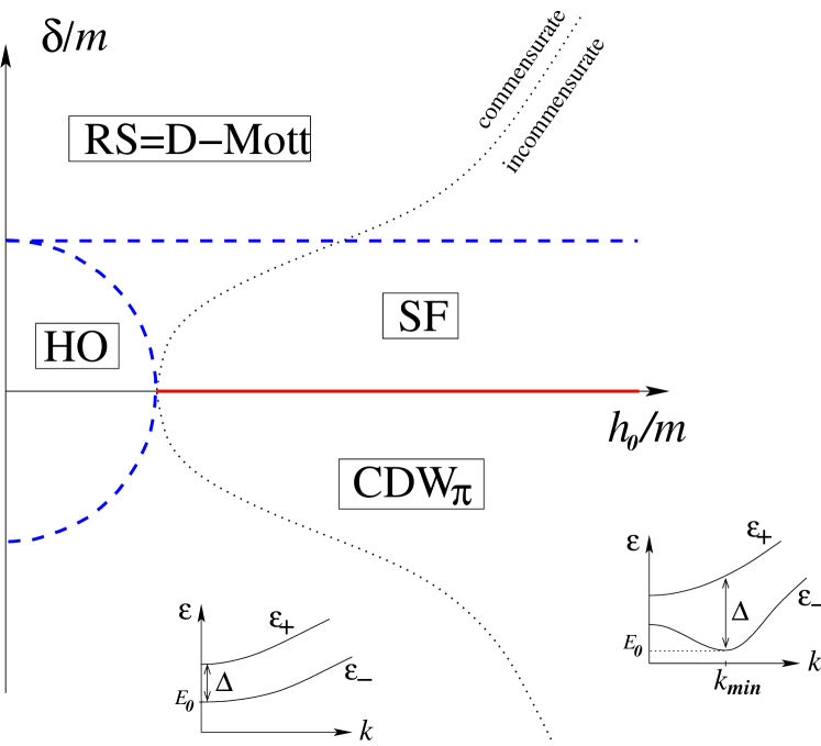
Figure 14: (Color online) Phase diagram of the generalized Hund ladder with interchain hopping. The coordinate on the horizontal axis is proportional to $t_{\perp}$ whereas that on the vertical axis is the distance $D_{o}$ to the SU(2) orbital symmetric model. Blue lines indicate $c=\frac{1}{2}$ critical lines, and the red one is a $c=1$ critical line. See the main text for the definition of the phases. The dashed line, with equation $m^{2}\delta^{2}=h_{o}^{2}(h_{o}^{2}-m^{2})$, indicates the location where incommensuration appears: on the right of this curve, the lower band $\epsilon_{-}$ displays a minimum for a wave vector $k_{min}$. The two insets display the typical spectrum in the commensurate and incommensurate regions, respectively.

To identify the phases of the ladder lying on both sides of those lines (see Fig. 14), one notices that by continuity with what happens at $t_{\perp}=0$, the phase with $m_{4}<0$ (obtained at large enough $\delta$) must be a RS phase (which coincides with the D-Mott phase). The phase at $m_{4}>0$ is readily identified by means of the duality transformation $\xi^{4}_{L}\to-\xi^{4}_{L}$ that amounts to $\Phi_{f}\leftrightarrow\sqrt{\pi}/2-\Theta_{f}$ (see Eqs. (75)): it is a SF phase.

By continuity with $t_{\perp}=0$, the pocket $\delta^{2}+h_{o}^{2}<m^{2}$ corresponds to a HO phase. The last phase to be mapped out is the one lying at $h_{o}^{2}+\delta^{2}>m^{2}$ and $\delta<0$: it is adiabatically connected to the ODW phase that one has obtained at $t_{\perp}=0$ and $D_{o}<0$ so that it is an ODW or CDW_π phase, as we named it in the context of the ladder with an interchain hopping.

C.2 Effective low-energy theory

We now make a qualitative connection with the weak-coupling analysis of Section III.4, which crucially relies on the existence of an extended $\widetilde{U(1)}$ symmetry in the orbital sector, and show that this symmetry is also emergent at low energy in the strong-coupling regime. In the strong-coupling limit, in the vicinity of the orbital symmetric line, the interchain hopping $t_{\perp}$ amounts to a magnetic field in orbital space, that will eventually drive the system to a incommensurate state: when $\delta=0$, as soon as $h_{o}>m$ the Fermi points shift to $k_{F}=\frac{\pi}{2a_{0}}+k^{*}$. Now if the “magnetic field” is large enough, i.e., if $k^{*}$ is large enough, this leaves the space for a low-energy description built on fields expanded around the new Fermi points. In this effective low-energy description, $4k_{F}$ umklapp terms have no effect as being strongly oscillating. This remains true if one departs from the orbital symmetric line $\delta=0$: in this case, the spectrum of the low energy band, $\epsilon_{-}(k)$, develops a gap but the incommensuration is still present in the form of a minimum (which becomes infinitely deep in the limit $h_{o}\gg m$) in $\epsilon_{-}(k)$ at a value $v_{o}k_{min}=\sqrt{h_{o}^{2}-m^{2}(1+\frac{\delta^{2}}{h_{o}^{2}})}$. This happens (see Fig. 14) when $\delta$ is small enough, $|\delta|<\delta_{c}=h_{o}\sqrt{\frac{h_{o}^{2}}{m^{2}}-1}$. But is there an associated emergent symmetry, as it was the case in the weak-coupling limit?

To investigate this, one has to enter into further details. Denoting by $A_{k}$ the unitary matrix diagonalizing $U_{k}$, with $A_{k}^{\dagger}U_{k}A_{k}=\mbox{Diag}(\epsilon_{-}(k),-\epsilon_{-}(k),\epsilon_{+}(k),-\epsilon_{+}(k))$, and introducing $\widetilde{\boldsymbol{\Psi}}_{k}=A_{k}^{-1}\boldsymbol{\Psi}_{k}=(\chi_{-}(k),\chi_{+}(k))$, one can represent in the eigenmode basis the orbital U(1) generators along $x$, $T^{x}_{tot,\pm}=i\int\,dx\,\left(\xi^{5}_{L}\xi^{6}_{L}\pm\xi^{5}_{R}\xi^{6}_{R}\right)=\int_{k>0}\widetilde{\boldsymbol{\Psi}}_{k}^{\dagger}T^{(\pm)}_{k}\widetilde{\boldsymbol{\Psi}}_{k}$. $T^{x}_{tot,\pm}$ are the total Noether charge and current. The Hermitian matrix elements $T^{(\pm)}_{k,\alpha\beta}$ are too cumbersome, and not particularly enlightening, to appear here, but the matrix $T^{(-)}_{k}$ has a remarkable block structure:

$$T^{(-)}_{k}=\left(\begin{array}[]{cc}t_{1}(k)\mathbb{I}&t_{2}(k)\sigma^{z}+t_{3}(k)\sigma^{x}\\ t_{2}(k)\sigma^{z}+t_{3}(k)\sigma^{x}&-t_{1}(k)\mathbb{I}\end{array}\right).$$ (99)

Let us now introduce two quantities characterizing the spectrum: the absolute minimum $E_{0}$ of the lower band, and the gap $\Delta$ from the minimum of the lower band $E_{0}$ to the upper band (see insets of Fig.14). Now, if the two bands $\epsilon_{+}(k)$ and $\epsilon_{-}(k)$ are well separated, i.e. if $\Delta\gg E_{0}$, it makes sense to describe the theory at low energies in terms of the two Majorana fermions $\chi_{-}(k)$. Introducing the projector $P^{-}$ that projects on this subspace, the effective Hamiltonian $H_{\rm eff}^{-}=P^{-}HP^{-}=\sum_{k}\epsilon_{-}(k)\chi_{-}^{\dagger}(k)\sigma_{z}\chi_{-}(k)$ commutes with $P^{-}\;T^{x}_{tot,-}\;P^{-}$. Thus, the total orbital current along $x$ is asymptotically conserved in the limit of large $\Delta/E_{0}$, and the low-energy theory is effectively $\widetilde{\mbox{U(1)}}$ symmetric. For a physical quantity computed in the low-energy, $\widetilde{\mbox{U(1)}}$-symmetric theory, violation of this emergent symmetry by processes connecting the two bands will result in corrections of order $(E_{0}/\Delta)^{2}$.

Now, the parameters $E_{0}$ and $\Delta$ bear qualitatively distinct forms in the commensurate and incommensurate regions. For simplicity, we restrict our attention to the case $h_{o}>m$. In the commensurate region, one has:

$$E_{0} = \sqrt{\delta^{2}+h_{o}^{2}}-m,$$

$$\Delta = 2m,$$ (100)

so that in general $E_{0}/\Delta$ is not small.

In contrast, in the incommensurate region, one has:

$$E_{0} = \delta\sqrt{1-\frac{m^{2}}{h_{o}^{2}}}\;\lesssim\;{\cal O}(\delta),$$

$$\Delta = \sqrt{4h_{o}^{2}+E_{0}^{2}}-E_{0},$$ (101)

so that the symmetry $\widetilde{\mbox{U(1)}}$ is violated by terms of order $(\delta/2h_{o})^{2}$: the symmetry $\widetilde{\mbox{U(1)}}$ is asymptotically exact in the limit $h_{o}\gg\delta$. One thus concludes that close to the line $J_{t}=-3J_{H}/4$, the situation at large coupling coincides with that at small coupling. One can thus reasonably infer that this symmetry is emergent in all regimes at least close to the line $J_{t}=-3J_{H}/4$. Our strong coupling analysis suggests that the emergent $\widetilde{\mbox{U(1)}}$ is broken when moving far away from the orbital symmetric line ; however, the question of the existence of such an emergent symmetry in the strong-coupling regime of the generic electronic two-leg ladder goes far beyond the scope of this paper.

References

- (1) S. Sachdev, Quantum Phase Transitions (Cambridge University Press, Cambridge, England, 1999).
- (2) T. Senthil, A. Vishwanath, L. Balents, S. Sachdev, M. P. A. Fisher, Science 303, 1490 (2004); T. Senthil, L. Balents, S. Sachdev, A. Vishwanath, and M. P. A. Fisher, Phys. Rev. B 70, 144407 (2004).
- (3) A. O. Gogolin, A. A. Nersesyan, and A. M. Tsvelik, Bosonization and Strongly Correlated Systems (Cambridge University Press, Cambridge, England, 1998).
- (4) T. Giamarchi, Quantum Physics in One Dimension (Clarendon press, Oxford, UK, 2004).
- (5) H.-H. Lin, L. Balents, and M. P. A. Fisher, Phys. Rev. B 58, 1794 (1998).
- (6) D. Scalapino, S.-C. Zhang, and W. Hanke, Phys. Rev. B 58, 443 (1998).
- (7) H. Frahm and M. Stahlsmeier, Phys. Rev. B 63, 125109 (2001).
- (8) K. Le Hur, Phys. Rev. B 63, 165110 (2001).
- (9) J. B. Marston, J. O. Fjaerestad, and A. Sudbo, Phys. Rev. Lett. 89, 056404 (2002).
- (10) J. O. Fjaerestad and J. B. Marston, Phys. Rev. B 65, 125106 (2002).
- (11) M. Tsuchiizu and A. Furusaki, Phys. Rev. B 66, 245106 (2002).
- (12) C. Wu, W. V. Liu, and E. Fradkin, Phys. Rev. B 68, 115104 (2003).
- (13) T. Momoi and T. Hikihara, Phys. Rev. Lett. 91, 256405 (2003).
- (14) R. Assaraf, P. Azaria, E. Boulat, M. Caffarel, and P. Lecheminant, Phys. Rev. Lett. 93, 016407 (2004).
- (15) M. Fabrizio and E. Tosatti, Phys. Rev. Lett. 94, 106403 (2005).
- (16) S. Lee, J. B. Marston, and J. O. Fjaerestad, Phys. Rev. B 72, 075126 (2005).
- (17) J. O. Fjaerestad, J. B. Marston, and U. Schollwöck, Ann. Phys. (NY) 321, 894 (2006).
- (18) J. E. Bunder and H.-H. Lin, Phys. Rev. B 79, 045132 (2009).
- (19) H.-H. Lin, Phys. Rev. B 58, 4963 (1998).
- (20) A. A. Nersesyan and A. M. Tsvelik, Phys. Rev. B 68, 235419 (2003)
- (21) S. T. Carr, A. O. Gogolin, and A. A. Nersesyan, Phys. Rev. B 76, 245121 (2007).
- (22) J. E. Bunder and H.-H. Lin, Phys. Rev. B 78, 035401 (2008).
- (23) F. D. M. Haldane, Phys. Lett. A 93, 464 (1983); Phys. Rev. Lett. 50, 1153 (1983).
- (24) T. Kennedy and H. Tasaki, Phys. Rev. B 45, 304 (1992).
- (25) D. G. Shelton, A. A. Nersesyan, and A. M. Tsvelik, Phys. Rev. B 53, 8521 (1996); A. A. Nersesyan and A. M. Tsvelik, Phys. Rev. Lett. 78, 3939 (1997), ibid. 79, 1171(E).
- (26) H. Watanabe, Phys. Rev. B 52, 12508 (1995); Y. Nishiyama, N. Hatano, and M. Suzuki, J. Phys. Soc. Jpn. 64, 1967 (1995); S. R. White, Phys. Rev. B 53, 52 (1996).
- (27) H. J. Schulz, cond-mat/9808167.
- (28) H. C. Lee, P. Azaria, and E. Boulat, Phys. Rev. B 69, 155109 (2004).
- (29) D. Controzzi and A. M. Tsvelik, Phys. Rev. B 72, 035110 (2005).
- (30) P. Lecheminant and K. Totsuka, Phys. Rev B 71, 020407(R) (2005); ibid. 74, 224426 (2006).
- (31) E. Boulat, P. Azaria, and P. Lecheminant, Nucl. Phys. B 822, 367 (2009).
- (32) D. P. Arovas and A. Auerbach, Phys. Rev. B 52, 10114 (1995).
- (33) T. Fukuhara, Y. Takasu, M. Kumakura, and Y. Takahashi, Phys. Rev. Lett. 98, 030401 (2007); S. Taie, Y. Takasu, S. Sugawa, R. Yamazaki, T. Tsujimoto, R. Murakami, and Y. Takahashi, arXiv:1005.3670.
- (34) A. V. Gorshkov, M. Hermele, V. Gurarie, C. Xu, P. S. Julienne, J. Ye, P. Zoller, E. Demler, M. D. Lukin, and A. M. Rey, Nature Physics 6, 289 (2010).
- (35) Y. Yamashita, N. Shibata, and K. Ueda, Phys. Rev. B 58, 9114 (1998).
- (36) S. K. Pati, R. R. P. Singh, and D. I. Khomskii, Phys. Rev. Lett. 81, 5406 (1998).
- (37) B. Frischmuth, F. Mila, and M. Troyer, Phys. Rev. Lett. 82, 835 (1999).
- (38) P. Azaria, A. O. Gogolin, P. Lecheminant, and A. A. Nersesyan, Phys. Rev. Lett. 83, 624 (1999); P. Azaria, E. Boulat, and P. Lecheminant, Phys. Rev. B 61, 12112 (2000).
- (39) C. Itoi, S. Qin, and I. Affleck, Phys. Rev. B 61, 6747 (2000).
- (40) C. Wu, J. P. Hu, and S. C. Zhang, Phys. Rev. Lett. 91, 186402 (2003).
- (41) P. Lecheminant, E. Boulat, and P. Azaria, Phys. Rev. Lett. 95, 240402 (2005); P. Lecheminant, P. Azaria, and E. Boulat, Nucl. Phys. B 798, 443 (2008).
- (42) C. Wu, Phys. Rev. Lett. 95, 266404 (2005).
- (43) D. Controzzi and A. M. Tsvelik, Phys. Rev. Lett. 96, 097205 (2006).
- (44) H.-H. Tu, G.-M. Zhang, and L. Yu, Phys. Rev. B 76, 014438 (2007); ibid. 74, 174404 (2006).
- (45) C. J. Wu, Mod. Phys. Lett. B 20, 1707 (2006).
- (46) S. Capponi, G. Roux, P. Azaria, E. Boulat, and P. Lecheminant, Phys. Rev. B 75, 100503(R) (2007).
- (47) S. Capponi, G. Roux, P. Lecheminant, P. Azaria, E. Boulat, and S. R. White, Phys. Rev. A 77, 013624 (2008).
- (48) G. Roux, S. Capponi, P. Lecheminant, and P. Azaria, Eur. Phys. J. B 68, 293 (2009).
- (49) Y. Jiang, J. Cao, and Y. Wang, EPL 87, 10006 (2009).
- (50) H. Nonne, P. Lecheminant, S. Capponi, G. Roux, and E. Boulat, Phys. Rev. B 81, 020408(R) (2010).
- (51) R. Assaraf, P. Azaria, M. Caffarel, and P. Lecheminant, Phys. Rev. B 60, 2299 (1999).
- (52) E. Szirmai, O. Legeza, and J. Solyom, Phys. Rev. B 77, 045106 (2008); K. Buchta, O. Legeza, E. Szirmai, J. Solyom, Phys. Rev. B 75, 155108 (2007).
- (53) J. Zhao, K. Ueda, and X. Wang, Phys. Rev. B 74, 233102 (2006).
- (54) S. Capponi, C. J. Wu, and S. C. Zhang, Phys. Rev. B 70, 220505 (2004).
- (55) S-C. Zhang, Science 275, 1089 (1997); E. Demler, W. Hanke, and S-C. Zhang, Rev. Mod. Phys. 76, 909 (2004).
- (56) S. R. White, Phys. Rev. Lett. 69, 2863 (1992); Phys. Rev. B 48, 10345 (1993); U. Schollwöck, Rev. Mod. Phys. 77, 259 (2005).
- (57) C. N. Yang, Phys. Rev. Lett. 63, 2144 (1989).
- (58) C. N. Yang and S. C. Zhang, Mod. Phys. Lett. B 4, 759 (1990); S.-C. Zhang, Int. J. Mod. Phys. B 5, 153 (1991).
- (59) P. W. Anderson, Phys. Rev. 112, 1900 (1958).
- (60) I. Affleck, D. P. Arovas, J. B. Marston, and D. A. Rabson, Nucl. Phys. B 366, 467 (1991).
- (61) A. V. Onufriev and J. B. Marston, Phys. Rev. B 59, 12573 (1999).
- (62) M. den Nijs and K. Rommelse, Phys. Rev. B 40, 4709 (1989).
- (63) E. H. Kim, G. Fáth, J. Sólyom, and D. J. Scalapino, Phys. Rev. B 62, 14965 (2000).
- (64) I. Affleck, T. Kennedy, E. H. Lieb, and H. Tasaki, Phys. Rev. Lett. 59, 799 (1987); Comm. Math. Phys. 115, 477 (1988).
- (65) T. Kennedy, J. Phys.: Condens. Matter 2, 5737 (1990).
- (66) P. Lecheminant and E. Orignac, Phys. Rev. B 65, 174406 (2002).
- (67) H. J. Schulz, Phys. Rev. B 34, 6372 (1986).
- (68) P. Di Francesco, P. Mathieu, and D. Sénéchal, Conformal Field Theory (Springer, Berlin, 1997).
- (69) D. Allen and D. Sénéchal, Phys. Rev. B 55, 299 (1997).
- (70) G. Mussardo, Statistical field theory: an introduction to exactly solved models in statistical physics (Clarendon press, Oxford, UK, 2009).
- (71) D. J. Gross and A. Neveu, Phys. Rev. D 10, 3235 (1974).
- (72) A. B. Zamolodchikov and Al. B. Zamolodchikov, Ann. Phys. (N.Y.) 120, 253 (1979).
- (73) F. H. L. Essler and R. M. Konik in From Fields to Strings: Circumnavigating Theoretical Physics, edited by M. Shifman, A. Vainshtein, and J. Wheather (World Scientific, Singapore, 2005); cond-mat/0412421.
- (74) M. Nakamura, Physica B 329-333, 1000 (2003).
- (75) E. Berg, E. G. Dalla Torre, T. Giamarchi, and E. Altman, Phys. Rev. B 77, 245119 (2008).
- (76) This phase is equivalent to the ODW phase for .
- (77) This phase is equivalent to the staggered dimerization phase (SPπ phase) that we have found for .
- (78) V. J. Emery and S. A. Kivelson, Phys. Rev. B 46, 10812 (1992).
- (79) S. Eggert and I. Affleck, Phys. Rev. B 46, 10866 (1992).
- (80) E. Wong and I. Affleck, Nucl. Phys. B 417, 403 (1994).
- (81) M. Fabrizio and A. O. Gogolin, Phys. Rev. B 51, 17827 (1995).
- (82) A. M. Tsvelik, Phys. Rev. Lett. 69, 2142 (1992).
- (83) A. M. Tsvelik, Phys. Rev. B 42, 10499 (1990).