Toward Fast Reliable Communication at Rates Near Capacity with Gaussian Noise

Abstract

For the additive Gaussian noise channel with average codeword power constraint, sparse superposition codes and adaptive successive decoding is developed. Codewords are linear combinations of subsets of vectors, with the message indexed by the choice of subset. A feasible decoding algorithm is presented. Communication is reliable with error probability exponentially small for all rates below the Shannon capacity.

I Introduction

Sparse superposition codes with computationally feasible decoding is shown to achieve exponentially small error probability for any rate below the capacity. A companion presentation [6] gives bounds for optimal least squares decoding.

Code construction is by linear combination of vectors of length $n$. Let $X_{1},X_{2},\ldots,X_{N}$ be a dictionary of such vectors. Organize it in a matrix $X$ of $N\!=\!BL$ columns, partitioned into $L$ sections of size $B$ a power of $2$. Codewords are superpositions $X\beta=\sum_{j}\beta_{j}X_{j}$ with each section having $1$ term non-zero. The set of such $\beta$ is not closed under linear combination, so these are not linear codes in the algebraic coding sense. Nevertheless, they are fast to code and decode.

The message is conveyed by the choice of the subset of $L$ terms, with one from each section. From an input bit string $u=(u_{1},u_{2},\ldots,u_{K})$, with $K=L\log_{2}B$, encoding is realized by regarding $u$ as a concatenation of $L$ numbers, each with $\log B$ bits, specifying the selected columns. The codewords $c=X\beta$ have power $(1/n)\sum_{i=1}^{n}c_{i}^{2}$, which will be near $P$ when averaged across the $2^{K}$ possible codewords. The received vector is $Y=X\beta+\epsilon$ with $\epsilon$ distributed N($0,\sigma^{2}I$).

A decoder maps the received vector into an estimate $\hat{u}$. With $sent=(j_{1},j_{2},\ldots,j_{L})$ being the terms sent, the decoder produces estimates $\hat{j}_{1},\hat{j}_{2},\ldots,\hat{j}_{L}$. Overall block error is the event $\hat{u}\neq u$ and section error is the event $\hat{j}_{\ell}\neq j_{\ell}$. The fraction of section mistakes is $(1/L)\sum_{\ell=1}^{L}1_{\{\hat{j}_{\ell}\neq j_{\ell}\}}$.

The reliability requirement is that the mistake rate is small with high probability or the block error probability is small, averaged over input strings $u$ as well as the distribution of $Y$. The supremum of reliable communication rates $R\!=\!K/n$ is the channel capacity $\mathcal{C}\!=\!(1/2)\log_{2}(1\!+\!P/\sigma^{2})$, as in [29], [11].

The challenge is to achieve arbitrary rates below the capacity, with reliable decoding in manageable computation time. Here communication rates are identified which are moderately close to the capacity and a fast decoding scheme is devised. It is demonstrated to have probability that is exponentially small in $L/(\log B)^{2}$ of there being more than a moderately small fraction of section mistakes.

The setting adopted is the discrete-time channel with real-valued inputs and outputs and independent Gaussian noise. Standard communication models have been reduced to this setting as in [17], [15], when there is a frequency band constraint with specified noise spectrum. Solution to the coding problem, married to appropriate modulation, is relevant to myriad settings involving transmission over wires or cables for internet, television, or telephone or in wireless radio, TV, phone, satellite or other space communications. Previous standard approaches, as discussed in [15], entail a decomposition into separate problems of modulation, of shaping of a multivariate signal constellation, and of coding. Though there are practical schemes with empirically good performance, theory for practical schemes achieving capacity is lacking. In our analysis, shaping is built directly into the code design.

The entries of $X$ are generated with the independent standard normal distribution. The coefficients are $\beta_{j}$ equal to $\sqrt{P_{(\ell)}}$ for $j=j_{\ell}$ in $sent$ and equal to $0$ otherwise, with sum of squares $\sum_{\ell=1}^{L}P_{(\ell)}=P$ matching the power constraint. In the simplest case, the same power is allocated to each section $P_{(\ell)}=P/L$. We also consider the choice of variable power with $P_{(\ell)}$ proportional to $e^{-2C\ell/L}$ and a slight variant of this allocation in which the power is variable across most $\ell$ and then levels for $\ell/L$ near $1$.

For a rate $R$ code, $nR=L\log B$, so the codelength $n$ and the subset size $L$ agree to within a log factor. Setting $L=B$ is sensible, or, for a target codelength $n$, one may set $B=n$ and $L=nR/\log n$. For the best case developed here, the rate $R$ is chosen to have a drop from capacity that is near $1/\log B$, to within a loglog factor. When the signal to noise ratio is large, one finds it desirable to arrange $\log B$ to be at least as large as $C$ to achieve at least a constant fraction of capacity.

Let’s summarize our findings. With constant power allocation, a two-step algorithm and a multi-step improvement reliably achieve rates up to a rate $R_{0}=(1/2)P/(P\!+\!\sigma^{2})$ less than capacity. With variable power and order $\log B$ steps, we bring the achievable rate up near capacity ${\mathcal{C}}$, albeit with a gap from capacity of order $1/\sqrt{\log B}$. With the variant in which the power is leveled for $\ell/L$ near $1$, the gap from capacity is reduced to order $1/\log B$, to within a loglog factor, and, moreover, the section mistake rate is less than a constant times $1/\log B$, except in an event of probability exponentially small in $L/(\log B)^{2}$, as we report here. Subsequent to the submission of this conference paper, we have refined this probability bound, obtaining that it is exponentially small in $L/(\log B)$, or equivalently $n/(\log n)^{2}$, to within a loglog factor, as will be reported in the upcoming journal submission.

The performance, as measured by the gap from capacity at a similar reliability level, is comparable to benchmarks of performance for schemes not demonstrated to be practical, including [6] for least squares decoding of related superposition codes, and [25] for theoretically optimal codes. For a gap from capacity of order $1/\log n$, the best error probability is exponentially small in $n/(\log n)^{2}$.

The decoder initially computes for the received $Y$, its inner product with the terms in the dictionary, and sees which are above a threshold. Such a set of inner products and comparisons is performed in parallel by a basic computational unit, e.g. a signal-processing chip with $N$ parallel accumulators, in time of order $n$. These are pipelined so that the inner products are updated in constant time as each element of $Y$ arrives.

The threshold, set high enough that incorrect terms are unlikely to be above threshold, leads to only a small fraction of terms decoded in any one such step. Additional steps are used to bring the total fraction decoded near $1$. These steps take the inner products with residuals of the fit from the terms previously above threshold. A variant of the inner product with residuals is found to be somewhat more amenable to analysis.

The decoder does not predetermine which sections are to be decoded on any one step, rather it adapts the choice in accordance with which has inner product observed to be above threshold. Thus we call it adaptive successive decoding.

We determine a function $g(x)$ mapping from $[0,1]$ into $[0,1]$, which has the role that if $x_{k-1}$ is a likely fraction of sections correctly decoded from previous steps up to $k\!-\!1$ then $g(x_{k-1})$, slightly adjusted, provides a value $x_{k}$ of total fraction of sections likely to be correctly decoded by step $k$. This function depends on the power allocation rule and the choice of rate. A choice of communication rate is acceptable if the function $g(x)$ is greater than $x$ over most of the interval. Such a function $g$ is said to be accumulative, allowing the succession of steps to build up a large fraction of correctly decoded sections, with only a small fraction of mistakes remaining. The role of $g(x)$ is illustrated in Figure $1$.

Our analysis provides summary formulas for the rate and the target fraction of mistakes that arise from bounding the extent of positivity of $g(x)-x$. These summary formulas provide proof of a favorable scaling of rate by our scheme for the particular reliability targets, indexed by the size of the code.

​​​​​​​

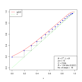
Figure 1: Plots of $g(x)$ and the sequence $x_{k}$. For $snr=15$ the plot takes $a=0.86$, $c=1.6$ and $\gamma=0.8C$ and the final false alarm and failed detection rates are $0.026$ and $0.013$ respectively, with probability bound of at least that fraction of mistakes equal to $0.002$. For $snr=1$, constant power allocation is used with $a=0.56$ and the false alarm and failed detection rates are $0.026$ and $0.053$ respectively, with probability bound $0.0007$.

Moreover, the function $g(x)$ can be evaluated in detail to choose settings of parameters ($a$, $c$, and $\gamma$ below). This allows computation of the best communication rate our analysis achieves, for given error probability and target mistake rates.

The parameter $a$ arises in the threshold $\tau=\sqrt{2\log B}+a$ of the standardized inner products. The parameter $c$ sets the height at which the variable power is leveled, with power $P_{(\ell)}$ chosen to be proportional to $\max\{e^{-2\mathcal{C}(\ell-1)/L},cut\}$, with $cut=e^{-2\mathcal{C}}(1\!+\!\delta_{c})$ where $\delta_{c}=c/\sqrt{2\log B}$.

Allowing power proportional to $\max\{e^{-2\gamma(\ell-1)/L},cut\}$, with $cut=e^{-2\gamma}(1\!+\!\delta_{c})$, for $\gamma$ between $0$ and $\mathcal{C}$, interpolates between the constant and variable cases.

Figure $2$ plots the rate $R$ as a function of $B$, from optimization of $a$, $c$, and $\gamma$, maintaining the bound $10^{-3}$ on the probability of a fraction of mistakes exceed $0.10$. Both the case $L=B$, and a large $L$ limit are shown as well as some results of simulation of the algorithm with $L=100$.

Signed superposition coding in which the $\ell$’th non-zero coefficient value is $\pm\sqrt{P_{(\ell)}}$ increases the number of codewords to $(2B)^{L}$ with the same reliability bounds, thereby improving the rate by a factor of $1+(\log 2)/(\log B)$, above what is shown in Figure 2. Arbitrary $L$ term subset coding (without partitioning) is possible, though not as simple, for a total rate improvement by a $1+(\log 2e)/(\log B)$ factor. For this presentation, we focus on the unsigned, partitioned superposition code case.

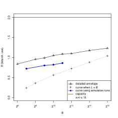
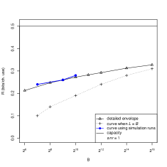
Figure 2: Curve showing achieved rates as a function of $B$ for $snr=15$ and $snr=1$. The x-axis has $B$ plotted on the $\log$ scale.

To prevent block errors, our subset superposition codes combine with error correction codes. The idea is to arrange sufficient distance between the subsets. Consider composition with an outer Reed-Solomon (RS) code of rate $1-2\delta$ near one, for an overall rate $(1\!-\!2\delta)R$. The alphabet of the RS code is taken to be of size $B$. Interpret its codewords as providing the sequence of labels $j_{1},j_{2},\ldots,j_{L}$ of the terms selected from the sections. The RS codelength $L$ is taken to be either $B-1$ or $B$ using a standard extension. RS code properties as in [24] guarantee correction of any fraction of section mistakes less than $\delta$. For advocacy of code concatenation see [14]. As a consequence of our result for the inner code, the composite code makes no mistakes, except in an event inheriting the exponentially small probability in $L/(\log B)^{2}$.

A fascinating alternative approach is channel polarization [2, 3], which achieves high rates for binary signaling with feasible decoding, with error probability exponentially small in $n^{1/2}$. For our scheme the error probability is exponentially small in $n^{1-\epsilon}$ for any $\epsilon\!>\!0$ and communication is permitted at higher rates beyond that associated with binary signalling.

Codes empirically demonstrated to be good include low density parity check codes and turbo codes, both with iterative statistical belief propagation decoding, but mathematically proof of performance near capacity is so far limited to special cases such as the binary erasure channel [22, 23].

Another approach to sparse superposition decoding is convex projection with $\ell_{1}$ constraint, arising from analogous problems of statistical learning and signal recovery. Iterative procedures and properties for such projection are in [19],[4],[21],[5], [18], with preliminary findings for communication in [30]. Each iteration would find in each section the term of highest inner product with the residuals and use it to update the convex combination. It is unclear to us whether convex projection for communication can be reliable at rates up to capacity.

The conclusions may be expressed in the language of sparse signal recovery. $L$ terms from a dictionary are linearly combined and subject to noise. For signals $X\beta$ recovery of the terms from the received noisy $Y$ is possible provided the number of observations $n$ is at least $(1/R)L\log B$. Recovery using $\ell_{1}$ constrained convex optimization is accurate provided $R\!<\!R_{0}$ in the equal power case. For our variable power designs, our results establish recovery by other means at higher $R\!<\!{\mathcal{C}}$. These findings complement work in [31],[32],[13],[12],[8], [26],[20]. For typical signal recovery problems there is greater freedom of design with non-zero coefficients values regarded as unknown, leading to bounds based on the minimum non-zero signal size, rather than exclusively based on the total signal power as in the communication capacity.

Superposition codes began with [10] for the broadcast channel, and later for multiple-access channels [9],[28]. Our purpose of computational feasibility is different from the original purpose of identifying the set of achievable rates. Another connection is the consideration of rate splitting and successive decoding. Our adaptive successive decoding yields feasibility in the single-user case and should work also in multi-user settings.

II The Decoder

From the received $Y$ and knowledge of the dictionary, decode which terms were sent by an iterative procedure. In the constant power allocation case set $P_{j}=P/L$. For the variable power case let $P_{j}=P_{(\ell)}$ for $j$ in section $\ell$.

First Step: For each term $X_{j}$ of the dictionary compute the statistic $\mathcal{Z}_{1,j}=X_{j}^{T}Y\,/\|Y\|$.The terms for which the statistic is above a threshold $\tau=\sqrt{2\log(B)}+a$ are regarded as decoded terms. Denote the associated event $\mathcal{H}_{j}=\{\mathcal{Z}_{1,j}\geq\tau\}$. The idea of the first step threshold is that very few of the terms not sent will be above threshold. Yet a positive fraction of the terms sent will be above threshold and hence will be correctly decoded on this first step, with an average likely to be at least a positive value $q$ as will be quantified.

Let $dec_{1}=\{j:1_{\mathcal{H}_{j}}=1\}$ be the set of terms decoded on this step. The first step provides the fit $F_{1}=\sum_{j}\sqrt{P_{j}}\,X_{j}1_{\mathcal{H}_{j}}$.

Second Step: For each of the remaining terms, form the inner product with the vector of residuals $r=Y-F_{1}$, that is, compute $X_{j}^{T}r$ or its normalized form $\mathcal{Z}_{j}^{r}=X_{j}^{T}r\,/\|r\|$. A quantity with similar properties is found to be equally easy to compute and somewhat simpler to analyze. Indeed, compute $F_{Y}=[F_{1}^{T}Y/\|Y\|^{2}]\,Y$ which is the part of $F_{1}$ in the direction $Y$ and the vector $G=F_{1}-F_{Y}$ which is the part orthogonal to $Y$. For each of the remaining $j$ compute $\mathcal{Z}_{2,j}=X_{j}^{T}G\,/\|G\|$. Then form the combined test statistic

$$\mathcal{Z}_{2,j}^{comb}\,=\,\sqrt{1\!-\!\lambda}\,\mathcal{Z}_{1,j}\,-\,\sqrt{\lambda}\,\mathcal{Z}_{2,j},$$

with $\lambda=q\,P/(\sigma^{2}\!+\!P)$. The specified $\lambda$ is chosen to maximize the mean separation between correct and wrong terms. For the two-step version, complete the decoding, in each section not previously decoded, by picking the term for which this statistic is largest, with no need for a second step threshold in that case.

Extension to Multiple Steps: We briefly describe how the algorithm is extended to multiple steps to provide increased reliability. The process initializes with $V_{1,j}=X_{j}$ the vectors of terms in the dictionary with index set $J_{1}$ consisting of all the terms. From the first step, $G_{1}=Y$ is the received vector and the statistics $\mathcal{Z}_{1,j}$ are $X_{j}^{T}G_{1}/\|G_{1}\|$ for $j$ in $J_{1}$ with associated events $\mathcal{H}_{1,j}=\mathcal{H}_{j}$.

For the second step the vector $G_{2}=G$ is formed, which is the part of $F_{1}$ orthogonal to $G_{1}=Y$. The set of terms investigated on this step is $J_{2}=J_{1}\cap\{j:1_{\mathcal{H}_{1,j}}=0\}$. For $j$ in $J_{2}$, the statistic $\mathcal{Z}_{2,j}=X_{j}^{T}G_{2}/\|G_{2}\|$ is computed as well as the combined statistic $\mathcal{Z}_{2,j}^{comb}=\sqrt{\lambda_{1}}\mathcal{Z}_{1,j}-\sqrt{\lambda_{2}}\mathcal{Z}_{2,j}$, where $\lambda_{1}=1-\lambda$ and $\lambda_{2}=\lambda$. What is different on the second step is consideration of the events $\mathcal{H}_{2,j}=\{\mathcal{Z}_{2,j}^{comb}\geq\tau\}$ with the same threshold $\tau$, leading to an additional part $F_{2}=\sum_{j\in J_{2}}\sqrt{P_{j}}\,X_{j}1_{\mathcal{H}_{2,j}}$ of the fit $F_{1}+F_{2}$. The second step provides some increase in separation, without attempting to resolve all in two steps.

Proceed, iteratively, to perform the following loop of calculations, for $k\geq 2$. From the output of step $k\!-\!1$, there is available the partial fit vector $F_{k-1}$ and for $k^{\prime}<k$ the previously stored vectors $G_{k^{\prime}}$ and statistics $\mathcal{Z}_{k^{\prime},j}$ at for $j$ in the previous set $J_{k-1}$. Plus there is a set $J_{k}$ of remaining terms for us to consider at step $k$. From the residual $r=Y-\hbox{fit}_{k-1}$, one may compute $\mathcal{Z}_{k,j}^{res}=X_{j}^{T}r/\|r\|$. Instead, for simplification of the analysis, compute the part $G_{k}$ of $F_{k-1}$ orthogonal to the previous $G_{k^{\prime}}$ and for each $j$ in $J_{k}$ compute

$$\mathcal{Z}_{k,j}=X_{j}^{T}G_{k}/\|G_{k}\|$$

and the combined statistic

$$\mathcal{Z}_{k,j}^{comb}=\sqrt{1-\lambda_{k}}\,\mathcal{Z}_{k-1,j}^{comb}-\sqrt{\lambda_{k}}\,\mathcal{Z}_{k,j},$$

where the value of $\lambda_{k}$ we shall specify is again chosen to maximize a measure of separation between correct and wrong terms. The statistics $\mathcal{Z}_{k,j}^{res}$ are similar, entailing empirically determined values of $\hat{\lambda}_{k}$. The statistics $\mathcal{Z}_{k,j}^{comb}$ are compared to the threshold, leading to the events $\mathcal{H}_{k,j}=\{\mathcal{Z}_{k,j}^{comb}\geq\tau\}$. The output of step $k$ is the vector

$$F_{k}=\sum_{j\in J_{k}}\sqrt{P_{j}}\,X_{j}1_{\mathcal{H}_{k,j}},$$

providing the update $\hbox{fit}_{k}=\hbox{fit}_{k-1}+F_{k}$. Also the vector $G_{k}$ and the statistics $\mathcal{Z}_{k,j}$ are appended to what was previously stored, at least for the terms $j$ in $J_{k}$. This step updates the set of decoded terms $dec_{k}$ to be $dec_{k-1}\cup\{j\in J_{k}:1_{\mathcal{H}_{k,j}}=1\}$ and updates the set of terms remaining for further consideration $J_{k+1}=\{j\in J_{k}:1_{\mathcal{H}_{k,j}}=0\}$. This completes the actions of step $k$ of the loop. The idea is that on each step $k$ we decode a substantial part of what remains, because of growth of the mean separation between terms sent and the others.

III Reliability

Let $\hat{q}_{k},\hat{f}_{k}$ be the fraction of correct detections and false alarms at step $k$. Also let $\hat{f}_{1,k}=\hat{f}_{1}+\ldots+\hat{f}_{k}$ be the total fraction of false alarms after $k$ steps. For the variable power case let $\pi_{j}=P_{j}/P$ and use $\hat{q}_{k}=\sum_{j\>sent\cap J_{k}}\pi_{j}\,1_{\mathcal{H}_{k,j}}$ and $\hat{f}_{k}=\sum_{j\>not\>sent\cap J_{k}}\pi_{j}\,1_{\mathcal{H}_{k,j}}$, as weighted fractions, relative to the total weight of terms sent.

It is not hard to see that $\hat{q}_{1,k}=\sum_{j\>sent}\pi_{j}\,1_{\mathcal{H}_{k,j}}$ is a lower bound on $\hat{q}_{1}+\!\ldots\!+\hat{q}_{k}$ the total weighted fraction of correct detections from steps $1$ to $k$.

Let’s specify a target false alarm rate $f^{*}$ that arise in our analysis for each step. For step $k$, for given $a>0$, set

$$f^{*}=\frac{1}{(\sqrt{2\log B}+a)\sqrt{2\pi}}\exp\{-a\sqrt{2\log B}-(1/2)a^{2}\}$$

and likewise set values $f>f^{*}$. Recall that the threshold $\tau=\sqrt{2\log B}+a$. Indeed, it is unlikely that $\hat{f}_{k}$ exceeds $f$.

Similarly, using distributional properties of $\hat{q}_{1,k}$ using the function $g(x)$ discussed below, we specify a value $q_{1,k}$ for which we expect that $\hat{q}_{1,k}$ is likely to be at least $q_{1,k}$. Further define, $x_{0}=0$ and for $k\geq 1$,

$$x_{k}=q_{1,k}^{adj}=\frac{q_{1,k}}{1+f_{1,k}/q_{1,k}},$$

where $f_{1,k}=kf$. These $x_{k}$ are used in setting the weight $\lambda_{k}$ and in expressing the mean separation $a_{k,j}$ between terms sent and terms not sent. Indeed $\lambda_{k}=w_{k}(1-x_{k}\nu)$ with

$$w_{k}=\frac{1}{1-x_{k}\nu}-\frac{1}{1-x_{k-1}\nu}$$

measuring the increase in a quantity used in specifying the separation. For establishing reliability, the critical matter is to demonstrate that $x_{k}=q_{1,k}^{adj}$ grows to a value near $1$. Define

$$\mu_{x}(u)=\left(\frac{\sqrt{u}}{\sqrt{1-x\nu}}-1\right)\sqrt{2\log B}-a^{\prime}.$$

Here $\nu=P/(\sigma^{2}+P)=1-e^{-2\mathcal{C}}$ and $a^{\prime}=a+h$, where $h$ is a small number positive number.

The $\mathcal{Z}_{k,j}^{comb}$ are not normally distributed, nevertheless, it is demonstrated by induction that in a set of high probability, they are greater than normal random variables which have mean $0$ for terms not sent and mean $a_{k,j}$ for terms sent. Across the terms $j$, the joint normal distribution that arises in this construction has a covariance $I-\nu_{k}\beta\beta^{T}/P$ where $\nu_{k}\leq\nu=P/(P+\sigma^{2})$, for which it is shown that the joint density is not more than a constant $1/(1-\nu)^{1/2}=e^{\mathcal{C}}$ times the joint density that would arise if they were independent standard normal.

In the constant power case with $R=R_{0}$, let $g(x)=\Phi(\mu_{x})$. where $\mu_{x}=\mu_{x}(1)$. Then for terms sent $a_{k,j}=-\mu_{x_{k-1}}$ and $q_{1,k}^{*}=g(x_{k-1})$ at $x_{k-1}=q_{1,k-1}^{adj}$. If $g(x)$ exceeds $x$, then there is room to set $q_{1,k}$ just below $q_{1,k}^{*}$, so that if $f_{1,k}=kf$ is small enough, then $x_{k}=q_{1,k}^{adj}$ is indeed larger than $x_{k-1}$.

The $g(x)-x$ stays above a positive $gap$ for all $0\!\leq\!x\!\leq\!x^{*}$. For the constant power case the positivity holds at $x^{*}$ provided $x^{*}$ is separated from $1$ by at least a polynomial in $1/B$, and this gap at $x^{*}$ is the minimum value in $[0,x^{*}]$ provided $a^{\prime}\leq\sqrt{2\pi}(.5-\bar{x}^{*})$ and $\Phi(-a^{\prime})\geq\bar{x}^{*}$ where $\bar{x}^{*}=1\!-\!x^{*}$.

Lemma 1: If $g(x)-x$ is at least a positive $gap$ on an interval $[0,x^{*}]$, choose small positive $\eta$ and $f>f^{*}$. Arrange $\Lambda=gap-\eta$ to be positive and for $4f\,x^{*}\leq\Lambda^{2}$ and arrange $q_{1,k}=q_{1,k}^{*}-\eta$ where $q_{1,k}^{*}=g(q_{1,k-1}^{adj})$. Then the increase on each step $q_{1,k}-q_{1,k-1}$ for which $q_{1,k-1}^{adj}\leq x^{*}$ is at least $\tilde{\Lambda}$, where $\tilde{\Lambda}$ satisfies $\tilde{\Lambda}=\Lambda-x^{*}\,f/\tilde{\Lambda}$, quadratic in $\tilde{\Lambda}$ with solution $\tilde{\Lambda}=\Lambda\{1+(1\!-\!4\,x^{*}\,f/\Lambda^{2})^{1/2}\}/2$. Moreover, the number of steps $m$ required such that on step $m-1$, the $q_{1,m-1}^{adj}$ first exceeds $x^{*}$, is bounded by $m\leq 1/\tilde{\Lambda}$ steps. At the final step $q_{1,m}$ exceeds $g(x^{*})-\eta$.

We also consider the variable power case. A quantity needed in our analysis is $C_{\ell,R}=\pi_{(\ell)}\,L\,\nu/2R$. With $\pi_{(\ell)}$ proportional to $u_{\ell}=e^{-2\mathcal{C}(\ell-1)/L}$, this $C_{\ell,R}$ becomes $u_{\ell}\,\mathcal{C}_{L}/R$, where the value $\mathcal{C}_{L}=(L/2)(1-e^{-2\mathcal{C}/L})$ is near the capacity $\mathcal{C}$. Then $C_{\ell,R}$ is near $u_{\ell}$ when $R$ is near the capacity $\mathcal{C}$. In the variable power case, the mean separation of the $\mathcal{Z}_{k,j}$ is given by $a_{k,j_{\ell}}=-\mu_{x}(C_{\ell,R})$ for section $\ell$. Likewise the role of the function $g(x)$ is played by

$$g_{L}(x)=\sum_{\ell=1}^{L}\pi_{(\ell)}\,\Phi(\mu_{x}(C_{\ell,R})).$$

When $\pi_{(\ell)}$ is proportional to $u_{\ell}=e^{-2\mathcal{C}(\ell-1)/L}$ this $g_{L}(x)$ is at least the value of a nearby integral

$$g(x)=\frac{1}{\nu}\int_{e^{-2C}}^{1}\Phi(\mu_{x}(u\mathcal{C}/R))\,du.$$

This $g(x)$ is found to compare favorably to $x$, to yield the required growth of the $x_{k}$.

Consider the case allowing leveling with which $\pi_{(\ell)}=\max\{u_{\ell},cut\}/sum$, for which the normalizing sum is found to be $(L\nu/2\mathcal{C})[1+\delta_{sum}^{2}]$, where $\delta_{sum}^{2}$ is near $D(\delta_{c})/snr$, bounded by $\delta_{c}^{2}/(2snr)$, with $\delta_{c}=c/\sqrt{2\log B}$ and $D(\delta)=(1\!+\!\delta)\log(1\!+\!\delta)-\delta$. The function $g_{L}(x)$ is defined as above with an analogous nearby integral with $\max\{u,cut\}$ in place of $u$. Set $r>0$ and consider the rate

$$R=\frac{\mathcal{C}}{(1+\delta_{sum}^{2})(1+\delta_{a})^{2}(1+2r/\tau_{B}^{2})},$$

where $\tau_{B}^{2}=2(\log B)(1\!+\!\delta_{a})^{2}$ with $\delta_{a}=a^{\prime}/\sqrt{2\log B}$. Setting a suitably small false alarm rate to not interfere with the accumulation of correct detections, the resulting $\delta_{a}$ is of order $[\log\log B+\log snr]/(\log B)$, so all three sources of rate drop above, $\delta_{sum}^{2}$, $\delta_{a}$ and $r/\tau_{B}^{2}$ are of order $1/\log B$ to within a loglog factor. A relevant lemma is the following.

Lemma 2: Let $x_{up}$ be near $1$ with $1-x_{up}=(1/snr)(2r/\tau_{B}^{2})$. For any non-negative $a$, $c$, and $r$, with the rate given above, the function $g(x)-x$ for $0\leq x\leq x_{up}$, is minimized at $x_{up}$.

The proof is based on an evaluation of the integral $g(x)$ which has expression in terms of the variable $z=\mu_{x}(cut\,\mathcal{C}/R)$ which is one-to-one with $x$. The value $x_{up}$ corresponds to a point $z_{up}=\zeta$ with favorable properties. Expressing the function in terms of $z$, one makes separate treatment of the behavior for $z\leq-\zeta$, where the function is close to decreasing, and for $-\zeta\leq z\leq+\zeta$, where the function is close to symmetric, slightly skewed to be lower at $+\zeta$.

The value of $\zeta$ is near $c/2$. Consider choices that approximately optimize the overall rate, yielding $\zeta$ near $\sqrt{\log_{+}((\log B)/4\pi)}$, at which the $gap$ of $g(x)-x$ at $x_{up}$ is at least a value near $(1/snr)(2r-1/2)/\tau_{B}^{2}$, positive for $r>1/4$. Moreover, choosing $a$ such that the false alarm rate $f=2f^{*}$ equals $(gap-\eta)^{2}/4$, so that the conditions of Lemma 1 are satisfied, it produces a value of $\delta_{a}$ of the indicated form.

Let’s state the result regarding reliability of the multi-step adaptive successive decoder. The proof is based on the above-mentioned normal approximation bound and a large deviation bound for weighted combinations of Bernoulli random variables, for which one may see the full manuscript [7].

Theorem 3: Suppose the communication rate and power allocation are such that $g$ is accumulative, with $g(x)-x>0$ on $[0,x^{*}]$. Pick $\eta_{k}=\eta$ and $f\!>\!f^{*}$ such that the conditions of Lemma 1 are satisfied, or more generally arrange $q_{1,k}=g(q_{1,k-1}^{adj})-\eta_{k}$ so that the increase $q_{1,k}-q_{1,k-1}$ remains positive for $k\!<\!m$. If the penultimate step $m\!-\!1$ is such that $q_{1,m-1}^{adj}$ is the first with value at least $x^{*}$, then with $rem=1-q_{1,m}$, the $m$ step single-dictionary decoder incurs a fraction of errors less than $mf+rem$, except in an event of probability not more than the sum for $k$ from $1$ to $m$ of

$$e^{-L_{\pi}D(q_{1,k}\|q_{1,k}^{*})+c_{0}k}+e^{-L_{\pi}(B\!-\!1)D(p\|p^{*})}+e^{-(n\!-\!k\!+\!1)D_{\epsilon_{k}}}.$$

Here $D(\cdot\|\cdot)$ refers to the Kullback-Leibler divergence between two Bernoulli random variables; $p,p^{*}$ equal the corresponding $f,f^{*}$ divided by $B\!-\!1$; and $D_{\epsilon}=-\log(1-\epsilon)-\epsilon$ which is at least $\epsilon^{2}/2$. Also $\epsilon_{k}=(n\epsilon\!-\!k\!+\!1)/(n\!-\!k\!+\!1)$, where $\epsilon=1-(1-h/\sqrt{2\log(B)}\,)^{2}$, and $c_{0}=\mathcal{C}$. Moreover, $L_{\pi}=1/\max_{\ell}\pi_{\ell}$, approximately a constant multiple of $L$ for the designs investigated here.

To produce each step $q_{1,k}$ from $q_{1,k}^{*}$, one may set a constant difference $\eta_{k}\!=\!\eta$ and invoke the bound $D(q_{1,k}\|q_{1,k}^{*})\geq 2\eta^{2}$. A preferred tactic, used in producing the curves shown earlier, is each step to choose $q_{1,k}$ to produce constancy of the exponent $D(q_{1,k}\|q_{1,k}^{*})$ at a prescribed value, equalizing the contributions to the above probability bound from each step.

References

- [1]
- [2] E. Arikan, “Channel polarization,” IEEE Trans. Inform. Theory, v.55, 2009.
- [3] E. Arikan and E. Telatar, “On the rate of channel polarization,” Preprint. ArXiv, Jul.2008.
- [4] A.R. Barron, “Universal approximation bounds for superpositions of a sigmoidal function,” IEEE Trans. Inform. Theory, v.39, 930-944, 1993.
- [5] A. Barron, A. Cohen, W. Dahmen and R. Devore, “Approximation and learning by greedy algorithms.” Ann. Statist. v.36, 64-94, 2007.
- [6] A.R. Barron, A. Joseph, “Least squares superposition coding of moderate dictionary size, reliable at rates up to channel capacity,” Proc. Internat. Symp. Inform. Theory, Austin, Texas, June 2010.
- [7] A.R. Barron, A. Joseph, “Fast Reliable Communication at Rates not Far from Capacity with Gaussian Noise,” Dept. Stat., Yale Univ.
- [8] E. Candes and Palm, “Near-ideal model selection by minimization,” Annals of Statistics, 2009.
- [9] J. Cao and E.M. Yeh, “Asymptotically optimal multiple-access cummincation via distributed rate splitting,” IEEE Trans. Inform. Theory, v.53, 304-319, Jan.2007.
- [10] T.M. Cover, “Broadcast channels,” IEEE Trans. Inform. Theory, v.18, 2-14, 1972.
- [11] T.M. Cover and J.A. Thomas, Elements of Information Theory, New York, Wiley-Interscience, 2006.
- [12] D.L. Donoho, M. Elad, and V.M. Temlyakov, “Stable recovery of sparse overcomplete representations in the presence of noise,” IEEE Trans. Inform. Theory, v.52, 6-18, Jan. 2006.
- [13] A.K. Fletcher, S. Rangan, and V.K. Goyal, “Necessary and sufficient conditions for sparsity pattern recovery,” IEEE Trans. Inform. Theory, v.55, 5758-5773, 2009.
- [14] G.D. Forney, Jr. Concatenated Codes, Research Monograph No.37, Cambridge, Massachusetts, M.I.T. Press. 1966.
- [15] G.D. Forney and G. Ungerboeck, “Modulation and coding for linear Gaussian channels,” IEEE Trans. Inform. Theory, v.44, Oct.1998.
- [16] R.G. Gallager, Low Density Parity-Check Codes, Cambridge, Massachusetts, M.I.T. Press. 1963.
- [17] R.G. Gallager, Information Theory and Reliable Communication, New York, John Wiley and Sons, 1968.
- [18] C. Huang, A.R. Barron, and G.H.L. Cheang, Preprint, 2008.
- [19] L. Jones, “A simple lemma for optimization in a Hilbert space, with application to projection pursuit and neural net training,” Annals of Statistics, v.20, 608-613, 1992.
- [20] A. Karbasi, A. Hormati, S. Mohajer, and M. Vetterli, “Support recovery in compressed sensiing: an estimation theoretic approach. IEEE Internat. Symp. Inform. Theory, 679-683, Seoul Korea, June 2009.
- [21] W.S. Lee, P. Bartlett, B. Williamson, IEEE Trans. Inform. Theory, 42, 2118-2132, 1996.
- [22] M.G. Luby, M. Mitzenmacher, M.A. Shokrollahi, and D.A. Spielman, “Efficient erasure correcting codes.” IEEE Trans. Inform. Theory, v.47, 569-584, Feb.2001.
- [23] M.G. Luby, M. Mitzenmacher, M.A. Shokrollahi, and D.A. Spielman, “Improved Low-Density Parity-Check Codes Using Irregular Graphs.” IEEE Trans. Inform. Theory, v.47, 585-598, Feb. 2001.
- [24] F.J. MacWilliams and N.J.A. Sloane, The Theory of Error-Correcting Codes, Amsterdam and New York, North-Holland Publishing Co.
- [25] Y. Polyanskiy, H.V. Poor, and S. Verdú, “Channel coding rate in the finite blocklength regime.” IEEE Trans. Inform. Theory. 2010.
- [26] K.R. Rad, “Sharp upper bound on error probability of exact sparsity recovery,” Proc. Conference Inform. Sciences Systems, 2009.
- [27] I.S. Reed and G. Solomon, “Polynomial codes over certain finite fields.” J. SIAM, v.8, 300-304, June 1960.
- [28] B. Rimoldi and R. Urbanke, “A rate-splitting approach to the Gaussian multiple-access channel capacity.” IEEE Trans. Inform. Theory, v.47, 364-375, Mar. 2001.
- [29] C.E. Shannon, “A mathematical theory of communication.” Bell Syst. Tech. J., v.27, 379-423 and 623-656, 1948.
- [30] J. Tropp, “Just relax: convex programming methods for identifying sparse signals in noise,” IEEE Trans. Inform. Theory, v.52, 1030-1051, Mar. 2006.
- [31] M.J. Wainwright, “Sharp thresholds for high-dimensional and noisy sparsity recovery using -constrained quadratic programming (Lasso).” IEEE Trans. Inform. Theory, v.55, 2183-2202, May 2009.
- [32] M.J. Wainwright, “Information-theoretic limits on sparsity recovery in the high-dimensional and noisy setting,” IEEE Trans. Inform. Theory, v.55, 5728-5741, Dec. 2009.