Generalized-ensemble simulations and cluster algorithms

Abstract

The importance-sampling Monte Carlo algorithm appears to be the universally optimal solution to the problem of sampling the state space of statistical mechanical systems according to the relative importance of configurations for the partition function or thermal averages of interest. While this is true in terms of its simplicity and universal applicability, the resulting approach suffers from the presence of temporal correlations of successive samples naturally implied by the Markov chain underlying the importance-sampling simulation. In many situations, these autocorrelations are moderate and can be easily accounted for by an appropriately adapted analysis of simulation data. They turn out to be a major hurdle, however, in the vicinity of phase transitions or for systems with complex free-energy landscapes. The critical slowing down close to continuous transitions is most efficiently reduced by the application of cluster algorithms, where they are available. For first-order transitions and disordered systems, on the other hand, macroscopic energy barriers need to be overcome to prevent dynamic ergodicity breaking. In this situation, generalized-ensemble techniques such as the multicanonical simulation method can effect impressive speedups, allowing to sample the full free-energy landscape. The Potts model features continuous as well as first-order phase transitions and is thus a prototypic example for studying phase transitions and new algorithmic approaches. I discuss the possibilities of bringing together cluster and generalized-ensemble methods to combine the benefits of both techniques. The resulting algorithm allows for the efficient estimation of the random-cluster partition function encoding the information of all Potts models, even with a non-integer number of states, for all temperatures in a single simulation run per system size.

1 Introduction

The Monte Carlo simulation method has developed into one of the standard tools for the investigation of statistical mechanical systems undergoing first-order or continuous phase transitions [1]. While the formulation of the Metropolis-Hastings algorithm [2, 3], which is the basic workhorse of the method up to this very day, dates back more than half a century ago, its initial practical value was limited. This was partially due to the the fact that computers for the implementation of such simulations where not widely available and the computing power of those at hand was very limited compared to today’s standards. Hence, the method was not yet competitive, e.g., for studying critical phenomena compared to more traditional approaches such as the $\epsilon$ or series expansions [4]. That the situation has changed rather drastically in favor of the numerical approaches since those times is not only owed to the dramatic increase in available computational resources, but probably even more importantly to the invention and refinement of a number of advanced techniques of simulation and data analysis. These include (but are not limited to) the introduction of the concept of finite-size scaling [5], which turned the apparent drawback of finite system sizes in simulations into a powerful tool for extracting the asymptotic scaling behavior, the invention of cluster algorithms [6, 7] beating the critical slowing down close to continuous transitions, the (re-)introduction of histogram reweighting methods [8, 9] allowing for the extraction of a continuous family of estimators of thermal averages from a single simulation run, and the utilization of a growing family of generalized-ensemble simulation techniques such as the multicanonical method [10], that allow to overcome barriers in the free-energy landscape and enable us to probe highly suppressed transition states.

In a general setup for a Monte Carlo simulation, the microscopic states of the system appear with frequencies according to a probability distribution $p_{\mathrm{sim}}(\{s_{i}\})$, which is an expression of the chosen prescription of picking states and hence specific to the used simulation algorithm. Here, having a spin system in mind, we label the states with the set $\{s_{i}\}$, $i=1,\ldots,V$, of variables. In thermal equilibrium, on the other hand, microscopic states are populated according to the Boltzmann distribution for the case of the canonical ensemble,

$$p_{\mathrm{eq}}(\{s_{i}\})=\frac{1}{Z_{\beta}}e^{-\beta{\cal H}(\{s_{i}\})},$$ (1)

where ${\cal H}(\{s_{i}\})$ denotes the energy of the configuration $\{s_{i}\}$ and $Z_{\beta}$ is the partition function at inverse temperature $\beta=1/T$. Therefore, any sampling prescription with non-zero probabilities for all possible microscopic states $\{s_{i}\}$ in principle allows to estimate thermal averages of any observable ${\cal O}(\{s_{i}\})$ from a time series $\{s_{i}^{(t)}\}$, $t=1,\ldots,N$, of observations,

$$\hat{O}=\frac{\displaystyle\sum_{t=1}^{N}{\cal O}(\{s_{i}^{(t)}\})\frac{\displaystyle p_{\mathrm{eq}}(\{s_{i}^{(t)}\})}{\displaystyle p_{\mathrm{sim}}(\{s_{i}^{(t)}\})}}{\displaystyle\sum_{t=1}^{N}\frac{\displaystyle p_{\mathrm{eq}}(\{s_{i}^{(t)}\})}{\displaystyle p_{\mathrm{sim}}(\{s_{i}^{(t)}\})}},$$ (2)

such that $O\equiv\langle{\cal O}\rangle=\langle\hat{O}\rangle$ at least in the limit $N\rightarrow\infty$ of an infinite observation time. For a finite number of samples, however, the estimate (2) becomes unstable as soon as the simulated and intended probability distributions are too dissimilar, such that only a vanishing number of simulated events are representative of the equilibrium distribution. This is illustrated in Fig. 1, where the distribution $p_{\mathrm{sim}}(\{s_{i}\})=\mathrm{const}.$ of purely random or simple sampling is compared to the canonical distribution (1) for a finite temperature $T$. Since the Boltzmann distribution (1) only depends on the energy $E={\cal H}(\{s_{i}\})$, it is here useful to compare the one-dimensional densities $p_{\mathrm{sim}}(E)$ and $p_{\mathrm{eq}}(E)$ instead of the high-dimensional distributions in state space. For importance sampling, on the other hand, the simulated probability density is identical to the equilibrium distribution which can be achieved, e.g., by proposing local updates $s_{i}\rightarrow s_{i}^{\prime}$ (spin flips) at random and accepting them according to the Metropolis rule

$$T(\{s^{\prime}_{i}\}|\{s_{i}\})=\min[1,p_{\mathrm{eq}}(\{s^{\prime}_{i}\})/p_{\mathrm{eq}}(\{s_{i}\})]$$ (3)

for the transition probability $T(\{s^{\prime}_{i}\}|\{s_{i}\})$.

Figure 1: Probability distributions of reduced energies $E\equiv{\cal H}/J$ for the example of a $16\times 16$ $2$-state Potts model at coupling $\beta J=0.4$, cf. Eq. (8). For the case of simple sampling, the overlap of $p_{\mathrm{sim}}(E)$ and $p_{\mathrm{eq}}(E)$ is vanishingly small, whereas the two distributions coincide exactly for the case of importance sampling.

While importance sampling is optimal in that the simulated and intended probability densities coincide, this benefit comes at the expense of introducing correlations between successive samples. Under these circumstances, the autocorrelation function of an observable ${\cal O}$ is expected to decay exponentially,

$$C_{\cal O}(t)\equiv\langle{\cal O}_{0}{\cal O}_{t}\rangle-\langle{\cal O}_{0}\rangle\langle{\cal O}_{t}\rangle\sim C_{\cal O}(0)e^{-t/\tau({\cal O})},$$ (4)

defining the associated autocorrelation time $\tau({\cal O})$. Autocorrelations are a direct limiting factor for the amount of information that be extracted from a time series of a given length for estimating thermal averages. This is most clearly seen by inspecting an alternative definition of autocorrelation time involving an integral or sum of the autocorrelation function,

$$\tau_{{\rm int}}({\cal O})\equiv\frac{1}{2}+\sum_{t=1}^{\infty}C_{\cal O}(t)/C_{\cal O}(0).$$ (5)

The resulting integrated autocorrelation time determines the precision of an estimate $\hat{O}$ for the thermal average $\langle{\cal O}\rangle$ from the time series [11],

$$\sigma^{2}(\hat{O})\approx\frac{\sigma^{2}({\cal O})}{N/2\tau_{\mathrm{int}}({\cal O})}.$$ (6)

The presence of autocorrelations hence effectively reduces the number of independent measurements by a factor $1/2\tau_{\mathrm{int}}({\cal O})$. Generically, autocorrelation times are moderate and the problem is thus easily circumvented by adapting the number of measurement sweeps according to the value of $\tau_{\mathrm{int}}$. The problem turns out to be much more severe, however, in the vicinity of phase transitions points. Close to a critical point, where clusters of pure phase states of all sizes constitute the typical configurations, one observes critical slowing down,

$$\tau\sim\min(\xi,L)^{z},$$ (7)

where the dynamical critical exponent $z$ is found to be close to $z=2$ for conventional local updating moves. Since the correlation length $\xi$ diverges as the transition is approached, the same holds true for the autocorrelation time. This problem is most elegantly solved by the introduction of cluster algorithms, which involve updating collective variables that happen to show incipient percolation right at the ordering transition of the spin system and, in addition, must exhibit geometrical properties which are commensurate with the intrinsic geometry of the underlying critical system. Such approaches are discussed for the case of the Potts model in the context of the random-cluster representation in Section 2.2 below.

Figure 2: Sampled probability distribution of the internal energy $E$ of the $q=20$ states Potts model on a $16\times 16$ square lattice at the transition coupling $\beta J=1.699669\ldots$

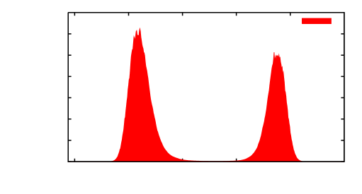
Even more dramatic correlation effects are seen for the case of first-order phase transitions. There, transition states connecting the pure phases coexisting at the transition are highly suppressed, leading to the phenomenon of metastability, where the phase of higher free energy persists in some region below the transition point for macroscopic times due to the free-energy barrier that needs to be overcome to effect the ordering of the system. This is illustrated in Fig. 2 displaying the order parameter distribution of a $q=20$ states Potts model. The mixed phase states connecting the peaks of the pure phases correspond to configurations containing interfaces and consequently carry an extra excitation energy $\sim 2\sigma L^{d-1}$, where $L$ denotes the linear size of the system and $\sigma$ is the surface free-energy per unit area associated to interfaces between the pure phases. The thermally activated dynamics in overcoming this additional energy barrier leads to exponentially divergent autocorrelation times,

$$\tau\sim\exp(-2\beta\sigma L^{d-1}),$$

sometimes referred to as hypercritical slowing down. Due to the finite correlation length at the transition point, cluster updates are of no use here but, instead, techniques for overcoming energy barriers are required. These can be provided (besides other means) by generalized-ensemble simulations discussed below in Section 3. Similar problems are encountered in simulations of disordered systems, where a multitude of metastable states separated by barriers is found [12].

The Potts model is a natural extension of the Ising model of a ferromagnet to a system with $q$-state spins and Hamiltonian

$${\cal H}=-J\sum_{\langle i,j\rangle}\delta(\sigma_{i},\sigma_{j}),\;\;\;\;\sigma_{i}=1,\ldots,q.$$ (8)

It is well known that the Potts model undergoes a continuous phase transitions for $q\leq 4$ in two dimensions and $q<3$ in three dimensions, while the transition becomes discontinuous for a larger number of states [13]. The $q=2$ Potts model is equivalent to the well-known Ising model. In the random-cluster representation introduced below in Section 2.2, the definition of the Potts model is naturally extended to all real values of $q>0$, and it turns out that the (bond) percolation problem then corresponds to the limit $q\rightarrow 1$, while for $q\rightarrow 0$ the model describes random resistor networks. Due to these properties, the Potts model serves as a versatile playground for the study of phase transitions with applications ranging from condensed matter to high-energy physics.

2 Using histograms

When studying phase transitions with Markov chain Monte Carlo simulations, one encounters another generic problem independent of the presence of autocorrelations. In the standard approach, estimators of the type (2) need to be used for each of a series of independent simulations at different values of the temperature (or other external parameters) to extract the temperature dependence of the observable at hand. This turns out to be problematic when studying phase transitions, where certain observables (such as, e.g., the specific heat) develop peaks which are narrowing down to the location of the transitions point as successively larger system sizes are considered. Locating such maxima to high precision then requires to perform a large number of independent simulation runs.

2.1 Energy and magnetization histograms

This problem is avoided by realizing that each time series from a simulation run at fixed temperature can be used to estimate thermal averages for nearby temperatures as well. The concept of histogram reweighting [8, 9] follows directly from the general relation (2) connecting simulated and target probability densities. If an importance sampling simulation is performed at coupling $K_{0}=\beta_{0}J$, i.e., $p_{\mathrm{sim}}\sim\exp(-K_{0}E)$, estimators for canonical expectation values at a different coupling $K$ are found from Eq. (2) with $p_{\mathrm{eq}}\sim\exp(-KE)$,

$$\hat{O}_{K}=\frac{\sum_{t=1}^{N}{\cal O}(\{s_{i}^{(t)}\})e^{-(K-K_{0}){\cal H}(\{s_{i}^{(t)}\})/J}}{\sum_{t=1}^{N}e^{-(K-K_{0}){\cal H}(\{s_{i}^{(t)}\})/J}}.$$ (9)

While this is conceptually perfectly general, it is clear that — quite similar to the case of simple sampling discussed above — reliable estimates can only be produced if the simulated and target distributions have significant overlap (cf. Figure 1). This is most clearly seen when switching over to a formulation involving histograms as estimates of the considered probability densities. If $\hat{H}_{K_{0}}(E)$ is a sampled energy histogram at coupling $K_{0}$ and the observable ${\cal O}$ only depends on the configuration $\{s_{i}\}$ via the energy $E$, the estimate (9) becomes

$$\hat{O}_{K}=\frac{\sum_{E}{\cal O}(E)\hat{H}_{K_{0}}(E)e^{-(K-K_{0})E}}{\sum_{E}\hat{H}_{K_{0}}(E)e^{-(K-K_{0})E}}.$$ (10)

It is useful to realize, then, that sampling the histogram $\hat{H}_{K_{0}}(E)$ one is, in fact, estimating the density of states $\Omega(E)$,

$$\langle\hat{H}_{K_{0}}(E)/N\rangle=p_{K_{0}}(E)=\frac{1}{Z_{K_{0}}}\Omega(E)e^{-K_{0}E}$$ (11)

i.e., the number of microstates of energy $E$ via

$$\hat{\Omega}(E)=Z_{K_{0}}\,\hat{H}_{K_{0}}(E)/N\times e^{K_{0}E},$$ (12)

where $Z_{K_{0}}$ denotes the partition function at coupling $K_{0}$. Inserting this expression into Eq. (11), one indeed arrives back at the reweighting estimate (10),

$$\hat{O}_{K}=\frac{1}{Z_{K}}\sum_{E}\hat{\Omega}(E)e^{-KE}{\cal O}(E)=\frac{Z_{K_{0}}}{Z_{K}}\sum_{E}\hat{H}_{K_{0}}(E)/N\times e^{-(K-K_{0})E}{\cal O}(E)$$ (13)

with

$$\widehat{\frac{Z_{K_{0}}}{Z_{K}}}=\frac{\sum_{E}\hat{H}_{K_{0}}(E)/N\times e^{-(K_{0}-K_{0})E}}{\sum_{E}\hat{H}_{K_{0}}(E)/N\times e^{-(K-K_{0})E}}.$$ (14)

It should be clear that the density of states is a rather universal quantity in that its complete knowledge allows to determine any thermal average related to the energy for arbitrary temperatures. The limitation in the allowable reweighting range, $|K-K_{0}|<\epsilon$, then translates into a window of energies for which the density of states $\Omega(E)$ can be reliably estimated from a single canonical simulation. This is illustrated in the left panel of Figure 3 for the $2$-state Potts model, where the density-of-states estimate of Eq. (12) from a single simulation at coupling $K=0.4$ is compared to the exact result. Note that from the estimator (12) $\Omega(E)$ can only be determined up to the unknown normalization constant $Z_{K_{0}}$. This is irrelevant for thermal averages of the type (10), but precludes the determination of free energies.

Figure 3: Density-of-states estimate $\hat{\Omega}(E)$ for the $2$-state Potts model on a $16\times 16$ square lattice from importance-sampling simulations at coupling $K=0.4$ (left panel) and from a series of simulations ranging from $K=0.1$ up to $K=0.9$ (right panel). The solid lines show the exact density of states calculated according to Ref. [14]. From the estimate (12) and the corresponding multi-histogram analogue (15), $\Omega(E)$ can only be determined up to an unknown normalization.

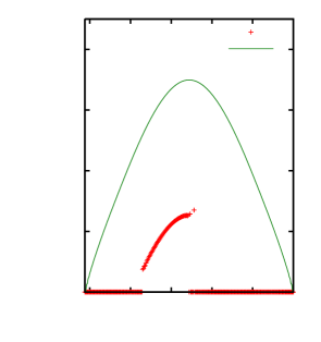
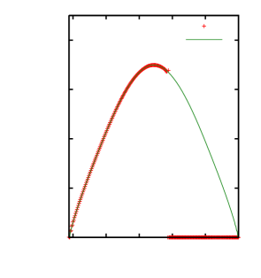
If more than a tiny patch of the domain of the density of states is to be determined, several simulations at different couplings $K$ need to be combined. Since the average internal energy increases monotonically with temperature, a systematic series of simulations can cover the relevant range of energies. A combination of several estimates of the form (12) for $\Omega(E)$ is problematic, however, since each estimate has a different, unknown scale factor $Z_{K_{i}}=e^{\cal F}_{i}$. This dilemma can be solved by the iterative solution of a system of equations. A convex linear combination of density-of-states estimates $\hat{\Omega}_{i}(E)$ from independent simulations at couplings $K_{i}$, $i=1,\ldots,n$,

$$\hat{\Omega}(E)\equiv\sum_{i=1}^{n}\alpha_{i}(E)\hat{\Omega}_{i}(E),$$

with $\sum_{i}\alpha_{i}(E)=1$ is of minimal variance for [15]

$$\alpha_{i}(E)=\frac{1/\sigma^{2}[\hat{\Omega}_{i}(E)]}{\sum_{i}1/\sigma^{2}[\hat{\Omega}_{i}(E)]}.$$

In view of Eq. (12), and ignoring the variance of the scale factors $e^{{\cal F}_{i}}$, one estimates

$$\sigma^{2}[\hat{\Omega}_{i}(E)]\approx e^{2{\cal F}_{i}}\hat{H}_{K_{i}}(E)/N^{2}\times e^{2K_{i}E},$$

such that

$$\hat{\Omega}(E)=\frac{\sum_{i}e^{-{\cal F}_{i}-K_{i}E}}{\sum_{i}e^{-2{\cal F}_{i}-2K_{i}E}[\hat{H}_{K_{i}}(E)/N]^{-1}}.$$ (15)

From Eq. (12) follows the normalization condition

$$e^{\cal F}_{i}=\sum_{E}\hat{\Omega}(E)e^{-K_{i}E},$$ (16)

which needs to be solved iteratively with Eq. (15) to simultaneously result in the optimized estimate $\hat{\Omega}(E)$ and the scale factors ${\cal F}_{i}$. An initial estimate can be deduced from thermodynamic integration [9, 16, 1]. Here, again, it is a crucial condition that the energy histograms to be combined have sufficient overlap. Otherwise, the iterative solution of Eqs. (15) and (16) cannot converge. Combining an appropriately chosen series of simulations, from this multi-histogram approach a reliable estimate of the full density of states can be achieved, as is illustrated in the right panel of Figure 3 for the case of the $2$-state Potts model. (The states to the right of the maximum in $\Omega(E)$ belong to the antiferromagnetic Potts model and thus are not seen in the simulations.) If the full range of admissible energies has been sampled, also an absolute normalization of $\Omega(E)$ becomes possible, matching $\hat{\Omega}(E)$ to reproduce the number $q$ of ground states or the number $q^{\cal N}$ of different states in total, where ${\cal N}$ denotes the number of Potts spins.

For estimating thermal averages of observables that do not depend on the energy only, the outlined framework can be easily generalized by replacing the measurements ${\cal O}(E)$ in Eq. (10) by the corresponding microcanonical averages $\langle{\cal O}\rangle_{E}$ at energy $E$,

$$\hat{O}_{K}=\frac{\sum_{E}\langle{\cal O}\rangle_{E}\hat{H}_{K_{0}}(E)e^{-(K-K_{0})E}}{\sum_{E}\hat{H}_{K_{0}}(E)e^{-(K-K_{0})E}}.$$

In the context of spin models, for instance, it can be useful to sample joint histograms of energy and magnetization and also define the corresponding two-dimensional density of states [17]. For the Potts model, however, it appears to be even more natural to consider a density of states occurring in the random cluster representation which also is the natural language for the formulation of cluster algorithms. This will be discussed in the next section.

2.2 Random cluster histograms

As was first noted by Fortuin and Kasteleyn [18], the partition function of the zero-field Potts model on a general graph ${\cal G}$ with ${\cal N}$ vertices and ${\cal E}$ edges can be rewritten as

$$Z_{K,q}\equiv\sum_{\{\sigma_{i}\}}e^{K\sum_{\langle i,j\rangle}\delta(\sigma_{i},\sigma_{j})}=\sum_{{\cal G}^{\prime}\subseteq{\cal G}}(e^{K}-1)^{b({\cal G}^{\prime})}\,q^{n({\cal G}^{\prime})},$$ (17)

where the sum runs over all bond configurations ${\cal G}^{\prime}$ on the graph (subgraphs). Note that the formulation (17) in contrast to that of Eq. (8) allows for a natural continuation of the model to non-integer values of $q$. This expression can be interpreted as a bond-correlated percolation model with percolation probability $p=1-e^{-K}$:

$$Z_{p,q}=e^{K{\cal E}}\sum_{{\cal G}^{\prime}\subseteq{\cal G}}p^{b({\cal G}^{\prime})}(1-p)^{{\cal E}-b({\cal G}^{\prime})}\,q^{n({\cal G}^{\prime})}=e^{K{\cal E}}\sum_{b=0}^{{\cal E}}\sum_{n=1}^{{\cal N}}g(b,n)\,p^{b}\,(1-p)^{{\cal E}-b}\,q^{n},$$ (18)

where $g(b,n)$ denotes the number of subgraphs of ${\cal G}$ with $b$ activated bonds and $n$ resulting clusters. This purely combinatorial quantity corresponds to the density of states of the random-cluster model.

It is this formulation of the model which is exploited by the cluster algorithms [6, 7] mentioned above. Since the Potts model is equivalent to a (correlated) percolation model, it follows (almost) automatically that the thus defined clusters percolate at the ordering transition and have the necessary fractal properties. This deep connection between spin model and percolation problem results in cluster algorithms for the Potts model dramatically reducing, and in some cases completely removing, the effect of critical slowing down [19]. It appears thus desirable to combine this extraordinarily successful approach with the idea of reweighting to result in continuous families of estimates. In particular, one would want to reweight in the temperature as well as the now continuous parameter $q$, for instance for determining the tricritical value $q_{c}$ where the transition becomes of first order. In contrast to previous attempts in this direction [20] using the language of energy and magnetization that results in certain systematic errors, such reweighting is very naturally possible in the random-cluster representation. By construction, a cluster-update simulation of the $q_{0}$-state Potts model at coupling $K_{0}$ produces bond configurations with the probability distribution

$$p_{p_{0},q_{0}}(b,n)=W_{p_{0},q_{0}}^{-1}\,g(b,n)\,p_{0}^{b}\,(1-p_{0})^{{\cal E}-b}\,q_{0}^{n},$$ (19)

where $p_{0}=1-e^{-K_{0}}$ and $W_{p_{0},q_{0}}\equiv Z_{p_{0},q_{0}}e^{-K_{0}{\cal E}}$. Therefore, if a histogram $\hat{H}_{p_{0},q_{0}}(b,n)$ of bond and cluster numbers is sampled, one has $p_{p_{0},q_{0}}(b,n)=\langle\hat{H}_{p_{0},q_{0}}(b,n)/N\rangle$ and thus follows an estimate of $g(b,n)$ as [16]

$$\hat{g}(b,n)=W_{p_{0},q_{0}}\frac{\hat{H}_{p_{0},q_{0}}(b,n)}{p_{0}^{b}\,(1-p_{0})^{{\cal E}-b}\,q_{0}^{n}\,N},$$ (20)

which, analogous to the estimate (12), contains an (unknown) normalization factor, $W_{p_{0},q_{0}}$. The required cluster decomposition of the lattice is a by-product of the Swendsen-Wang update and hence its determination does not entail any additional computational effort.

In this way, cluster-update simulations with largely reduced critical slowing down can be used for a systematic study of the model for arbitrary temperatures and (non-integer) numbers of states. Thermal averages of observables ${\cal O}(b,n)$ can be easily deduced from $\hat{g}(b,n)$,

$$\hat{\cal O}(p,q)\equiv\left[{\cal O}\right]_{p,q}=\frac{\displaystyle\sum_{b=0}^{{\cal E}}\sum_{n=1}^{{\cal N}}\hat{H}_{p_{0},q_{0}}(b,n)\left(\frac{p}{p_{0}}\right)^{b}\left(\frac{1-p}{1-p_{0}}\right)^{{\cal E}-b}\left(\frac{q}{q_{0}}\right)^{n}{\cal O}(b,n)}{\displaystyle\sum_{b=0}^{{\cal E}}\sum_{n=1}^{{\cal N}}\hat{H}_{p_{0},q_{0}}(b,n)\left(\frac{p}{p_{0}}\right)^{b}\left(\frac{1-p}{1-p_{0}}\right)^{{\cal E}-b}\left(\frac{q}{q_{0}}\right)^{n}}.$$ (21)

Relating expressions in the $(b,n)$ and $(E,M)$ languages, we have,

$$\hat{u} = -\frac{1}{p{\cal N}}\,[b]_{p,q},$$

$$\hat{c}_{v} = \frac{K^{2}}{p^{2}{\cal N}}\,\left(\left[(b-[b]_{p,q})^{2}\right]_{p,q}-(1-p)[b]_{p,q}\right),$$

where $u$ denotes the internal energy per spin and $c_{v}$ is the specific heat. For magnetic observables, an additional distinction between percolating and finite clusters is necessary [16].

Figure 4: Random-cluster density of states $g(b,n)$ on the $16\times 16$ square lattice as estimated from a Swendsen-Wang cluster-update simulation of the $q=2$ Potts model at $K=0.8$ (left panel) and the $q=2$ (brighter part, below) as well as $q=10$ (darker part, on top) models at a range of different couplings (right panel). Brighter colors correspond to larger values of $\hat{g}(b,n)$. The white areas correspond to $(b,n)$ values not visited in the simulations.

For averages at general values of $p$ and $q$, we run into the by now familiar problem of vanishing overlap of histograms as we move too far from the simulated $(p_{0},q_{0})$ point. This is illustrated in Figure 4, showing the support of the density-of-states estimate $\hat{g}$ in the $(b,n)$ plane. For a single canonical simulation, only a small patch of the $(b,n)$ plane is sampled (left panel). To improve on this, a multi-histogramming approach analogous to the technique discussed in the previous section is required. The relations corresponding to Eqs. (15) and (15) are here [16]

$$\hat{g}(b,n)=\frac{\sum_{i}N_{i}\,e^{-{\cal F}_{i}}\,p_{i}^{b}\,(1-p_{i})^{{\cal E}-b}\,q_{i}^{n}}{\sum_{j}N_{j}^{2}\,e^{-2{\cal F}_{j}}\,p_{j}^{2b}\,(1-p_{j})^{2({\cal E}-b)}\,q_{j}^{2n}[\hat{H}_{p_{i},q_{i}}(b,n)]^{-1}},$$ (22)

and the following self-consistency equation for the free-energy factors ${\cal F}_{i}$:

$$e^{{\cal F}_{i}}=\sum_{b=0}^{\cal E}\sum_{n=1}^{\cal N}\hat{g}(b,n)\,p_{i}^{b}\,(1-p_{i})^{{\cal E}-b}\,q_{i}^{n}.$$ (23)

Combining a number of simulations at different temperatures and $q$ values, a more significant patch of the density of states $g(b,n)$ can thus be sampled, cf. the right panel of Figure 4. Note that in the $(b,n)$ plane, moving from $b=0$ to $b={\cal E}$ corresponds to moving from infinite to zero temperature, whereas increasing the number of states $q$ moves the histograms up along the $n$ axis, corresponding to the fact that the presence of more states will tend to produce configurations broken down into smaller (and thus more) clusters.

3 Generalized ensembles

Two problems arise for an estimate of the total random-cluster density of states $g(b,n)$ with the multi-histogram approach outlined above: (i) while simulations at sufficiently small $q$ profit from the application of cluster algorithms in that critical slowing down is strongly reduced, in the first-order regime of large $q$ cluster algorithms are not useful for tackling the hypercritical slowing down observed there and (ii) as the system size is increased, histograms from simulations at different (integer) values of $q$ cease to overlap, such that the set (22) and (23) of multi-histogram equations eventually breaks down. While the second problem could, in principle, be avoided by using the cluster algorithm suggested in Ref. [21] for general, non-integer $q$ values, we find it more convenient to tackle both issues simultaneously by moving away entirely from the concept of canonical simulations which, as it turns out, entails further advantages for the sampling problem.

The idea of multicanonical [10] (or, less specifically, generalized ensemble) simulations is motivated by the problem of dynamically tunneling the area of (exponentially) low probability in between the coexisting phases at a first order transition, cf. Figure 2. Instead of simulating the canonical distribution (1), consider importance sampling according to a generalized probability density,

$$p_{\mathrm{muca}}(E)=\frac{\Omega(E)/W(E)}{Z_{\mathrm{muca}}}=\frac{e^{S(E)-\omega(E)}}{Z_{\mathrm{muca}}},$$ (24)

where $W(E)$ resp. $\omega(E)$ denote (logarithms of) suitably chosen weight factors and $S(E)=\ln\Omega(E)$ is the microcanonical entropy. To overcome barriers, the sampling distribution should be broadened with respect to the canonical one, in the extremal case to become completely flat, $p_{\mathrm{muca}}(E)=\mathrm{const}$. For this case Eq. (24) tells us that

$$W(E)=\Omega(E)\;\;\;\text{resp.}\;\;\;\omega(E)=S(E).$$

Hence, we arrive back at the task of estimating the density of states of the system! Since $\Omega(E)$ is not known a priori, one needs to revert to a recursive solution, where starting out, e.g., with the initial guess $W_{0}(E)=1$ (corresponding to a canonical simulation at infinite temperature) one produces an estimate $\hat{\Omega}_{1}(E)$ of the density of states according to Eq. (12) and sets $W_{1}(E)=\hat{\Omega}_{1}(E)$. Repeating this process, eventually a reliable estimate for $\Omega(E)$ over the full range of energies can be produced. Note that with the help of the general relation (2) we can come back to estimating canonical averages at any time during the multicanonical iteration. An alternative, rather efficient, approach for arriving at a working estimate of $\Omega(E)$ was suggested in Ref. [23], where the weights $\omega(E)$ are continuously updated $\omega(E)\rightarrow\omega(E)+\phi$ after visits of the energy $E$, and the constant $\phi$ is gradually reduced to zero after the relevant energy range has been sufficiently sampled. Although such a prescription ceases to form an equilibrium Monte Carlo simulation, convergence to the correct density of states can be shown under rather general circumstances [24].

Some combinations of the successful concepts of cluster algorithms/representations and generalized-ensemble simulations have been suggested before, most notably the multibondic algorithm of Ref. [25], which attaches generalized weights to the bond distribution function only (see also Ref. [26]). Although it appears most natural, it seems that it has not been noticed before that multicanonical weights can be attached, instead, to the full random-cluster probability density (19) to directly estimate the geometrical density of states $g(b,n)$. In this “multi-bondic-and-clusteric” version one writes

$$p_{\mathrm{mubocl}}(b,n)=W_{\mathrm{mubocl}}^{-1}\,g(b,n)\,e^{-\gamma(b,n)},$$ (25)

such that the generalized weights $\exp[-\gamma(b,n)]$ lead to a completely flat histogram for $\gamma(b,n)=\ln g(b,n)$. At this point, it is crucial to observe that, since $g(b,n)$ is a purely combinatorial quantity describing the number of decompositions of the lattice through a given number of activated links, it is no longer necessary to simulate the underlying spin model and, instead, one can consider the corresponding percolation problem directly. This approach proceeds by simulating subgraphs ${\cal G}^{\prime}$ with local updates: assume that the current subgraph consists of $b$ active bonds resulting in a decomposition of the graph into $n$ clusters. Picking a bond of the graph ${\cal G}$ at random two local moves are possible:

1. If the chosen bond is not active, try to activate it. Then either

   1. activating the bond does not change the cluster number $n$ (internal bond), leading to a transition $(b,n)\rightarrow(b+1,n)$,

   2. or activating the bond does join two previously disjoint clusters (coordinating bond), such that $(b,n)\rightarrow(b+1,n-1)$.

2. If the chosen bond is already active, try to deactivate or delete it. Then either

   1. deleting the bond does not change the cluster number $n$ (internal bond), resulting in the transition $(b,n)\rightarrow(b-1,n)$,

   2. or deleting the bond breaks a cluster apart in two parts (coordinating bond), such that $(b,n)\rightarrow(b-1,n+1)$.

While with a naive approach (such as the application of the Hoshen-Kopelman algorithm [27]) most of these moves would be very expensive computationally, this is not the case for a clever choice of data structures and algorithms. We use so-called “union-find algorithms” with additional improvements known as balanced trees and path compression [28]. With these structures, the computational effort for identifying whether an inactive bond is internal or coordinating and, for case (1b), the amalgamation of two clusters are operations in constant running time, irrespective of the size of the graph (up to logarithmic correction terms). The decision whether an active bond is internal or coordinating, although an operation with ${\cal O}({\cal E})$ complexity in the worst case, can be implemented very efficiently with interleaved breadth-first searches. Only the operation (2b) of actually decomposing a cluster can be potentially expensive, but this is only a problem directly at the percolation threshold. These local steps are used for a generalized-ensemble simulation, for instance using the iteration suggested by Wang and Landau [23] to arrive at an estimate $\hat{g}(b,n)$ for the random-cluster density of states (additional speedups can be achieved employing interpolation schemes for yet unvisited $(b,n)$ bins).

Figure 5: Logarithm of the cluster density of states $g(b,n)$ of the $q$-state Potts model on a $16\times 16$ square lattice.

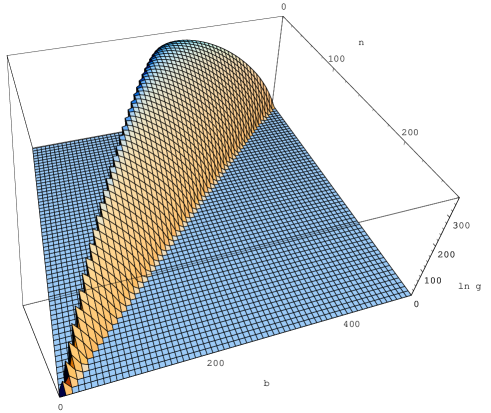
The estimated $g(b,n)$ can then be used either for directly estimating thermal averages via the relation (18) or as weight function for a multi-bondic-and-clusteric simulation to yield estimates of arbitrary observables via the general relation (2). Note that, by construction, the approach does not suffer from any (hyper-)critical slowing down, since it is based entirely on simulating a non-interacting percolation model. Figure 5 shows the (logarithm of the) density of states $g(b,n)$ sampled with this approach on a $16\times 16$ square lattice. While the $\hat{g}(b,n)$ resulting from this approach still comes only up to an unknown normalization constant, the random-cluster approach has the advantage that there exist ${\cal E}$ independent normalization conditions

$$g(b)=\sum_{n}g(b,n)\stackrel{{\scriptstyle!}}{{=}}{{\cal E}\choose b}.$$ (26)

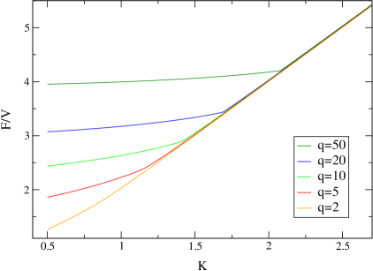
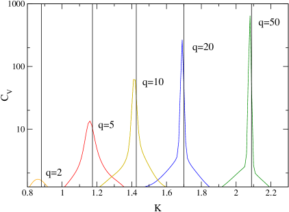
It is easily shown that the estimates from this approach reproduce the known results, e.g., for the internal/free energy and specific heat [29] or the (energy) density of states of the Ising model [14]. Beyond that, it is easy from this approach to study Potts model properties as a continuous function of $q$, or to study equilibrium distributions of Potts models with a large number of states without the problem of hypercritical slowing down. This is illustrated in Figure 6.

Figure 6: Absolute free energy (left) and specific heat (right) of the $q=2$, $5$, $10$, $20$ and $50$ states Potts model on a $16\times 16$ square lattice as estimated from the density of states $\hat{g}(b,n)$ resulting from a “multi-bondic-and-clusteric” simulation described in the main text.

4 Conclusions

While importance sampling Monte Carlo simulations according to the Metropolis-Hastings scheme appear to be the universally optimal solution to the problem of estimating equilibrium thermal averages, a number of complications are encountered in practical applications which result (a) from the requirement of computing estimates as continuous functions of external parameters and (b) the Markovian nature of the algorithm entailing autocorrelations that can lead to dynamic ergodicity breaking. I have outlined how a number of techniques such as histogram reweighting, cluster algorithms and generalized-ensemble simulations can provide (partial) solutions to these problems. It turns out that all of these techniques are closely related to the problem of estimating the density of states of the model at hand which turns out to be a central quantity for the understanding of advanced simulation techniques. For the prototypic case of the Potts model, it is shown how a combination of the random-cluster representation underlying the concept of cluster algorithms and multicanonical simulations allows to reduce the simulation to a purely geometric cluster counting problem that can be efficiently solved, e.g., with the Wang-Landau sampling scheme to yield arbitrary thermal averages as continuous functions of both the temperature and the (general, non-integer) number of states $q$. Possible applications are investigations of the tricritical point in the $(T,q)$ plane, estimates of critical exponents as continuous functions of $q$, or the investigation of transition states in the first-order regime, to name only a few of the problems that immediately come to mind.

References

- [1] K. Binder and D. P. Landau, A Guide to Monte Carlo Simulations in Statistical Physics, 2nd edn. (Cambridge University Press, Cambridge, 2005).
- [2] N. Metropolis, A. W. Rosenbluth, M. N. Rosenbluth, A. H. Teller, and E. Teller, J. Chem. Phys. 21 (1953) 1087.
- [3] W. K. Hastings, Biometrika 57 (1970) 97.
- [4] J. Zinn-Justin, Quantum Field Theory and Critical Phenomena, 4th edn. (Oxford University Press, Oxford, 2002).
- [5] M. E. Barber, in Phase Transitions and Critical Phenomena, eds. C. Domb and J. L. Lebowitz, vol. 8 (Academic Press, New York, 1983), p. 146.
- [6] R. H. Swendsen and J.-S. Wang, Phys. Rev. Lett. 57 (1986) 2607.
- [7] U. Wolff, Phys. Rev. Lett. 62 (1989) 361.
- [8] A. M. Ferrenberg and R. H. Swendsen, Phys. Rev. Lett. 61 (1988) 2635.
- [9] A. M. Ferrenberg and R. H. Swendsen, Phys. Rev. Lett. 63 (1989) 1195.
- [10] B. A. Berg and T. Neuhaus, Phys. Rev. Lett. 68 (1992) 9.
- [11] A. D. Sokal, in Quantum Fields on the Computer, ed. M. Creutz (World Scientific, Singapore, 1992), p. 211.
- [12] Y. Holovatch, ed., Order, Disorder and Criticality, vol. 1 and 2 (World Scientific, Singapore, 2007).
- [13] F. Y. Wu, Rev. Mod. Phys. 54 (1982) 235.
- [14] P. D. Beale, Phys. Rev. Lett. 76 (1996) 78.
- [15] M. Weigel and W. Janke, Phys. Rev. Lett. 102 (2009) 100601.
- [16] M. Weigel, W. Janke, and C.-K. Hu, Phys. Rev. E 65 (2002) 036109.
- [17] S.-H. Tsai and D. P. Landau, Phase diagram of a two-dimensional large- Potts model in an external field, Athens preprint.
- [18] C. M. Fortuin and P. W. Kasteleyn, Physica 57 (1972) 536.
- [19] W. Janke, in Computational Physics, eds. K. H. Hoffmann and M. Schreiber (Springer, Berlin, 1996), p. 10.
- [20] J. Lee and J. M. Kosterlitz, Phys. Rev. B 43 (1991) 1268.
- [21] L. Chayes and J. Machta, Physica A 254 (1998) 477.
- [22] B. Berg, J. Stat. Phys. 82 (1996) 323.
- [23] F. Wang and D. P. Landau, Phys. Rev. Lett. 86 (2001) 2050.
- [24] C. Zhou and R. N. Bhatt, Phys. Rev. E 72 (2005) 025701.
- [25] W. Janke and S. Kappler, Phys. Rev. Lett. 74 (1995) 212.
- [26] A. K. Hartmann, Phys. Rev. Lett. 94 (2005) 050601.
- [27] J. Hoshen and R. Kopelman, Phys. Rev. B 14 (1976) 3438.
- [28] M. E. J. Newman and R. M. Ziff, Phys. Rev. E 64 (2001) 016706.
- [29] A. E. Ferdinand and M. E. Fisher, Phys. Rev. 185 (1969) 832.