Compactons and semi-compactons in the extreme baby Skyrme model

Abstract

The static baby Skyrme model is investigated in the extreme limit where the energy functional contains only the potential and Skyrme terms, but not the Dirichlet energy term. It is shown that the model with potential $V=\frac{1}{2}(1+\varphi_{3})^{2}$ possesses solutions with extremely unusual localization properties, which we call semi-compactons. These minimize energy in the degree 1 homotopy class, have support contained in a semi-infinite rectangular strip, and decay along the length of the strip as $x^{-\log x}$. By gluing together several semi-compactons, it is shown that every homotopy class has linearly stable solutions of arbitrarily high, but quantized, energy. For various other choices of potential, compactons are constructed with support in a closed disk, or in a closed annulus. In the latter case, one can construct higher winding compactons, and complicated superpositions in which several closed string-like compactons are nested within one another. The constructions make heavy use of the invariance of the model under area-preserving diffeomorphisms, and of a topological lower energy bound, both of which are established in a general geometric setting. All the solutions presented are classical, that is, they are (at least) twice continuously differentiable and satisfy the Euler-Lagrange equation of the model everywhere.

1 Introduction

Solitons are stable, spatially localized solutions of nonlinear field theories. Ordinarily, “spatially localized” means that the field $\varphi(t,x)$ approaches some constant vacuum value $\varphi_{0}$ asymptotically as $|x|\rightarrow\infty$, usually exponentially in $|x|$ (e.g. KdV and sine-Gordon solitons, abelian Higgs vortices) sometimes as a power law $|x|^{-p}$ (e.g. sigma model lumps, instantons). However, there are some systems where the solitons’ spatial localization is much more severe: $\varphi(x)=\varphi_{0}$ exactly outside some compact region of space. Since they have compact support, these solitons are called compactons in the literature. They were first discovered in generalized KdV equations [8], then in nonlinear Klein-Gordon models with W-shaped potentials [3], that is, potentials with two degenerate vacua at each of which the potential has a V-shaped singularity. All these compactons live in one (spatial) dimension. Moving to two dimensions, compactons have been constructed for the baby-Skyrme model, with energy density

$$\mathscr{E}=\frac{1}{2}\lambda\partial_{i}\varphi\cdot\partial_{i}\varphi+\frac{1}{4}(\partial_{i}\varphi\times\partial_{j}\varphi)\cdot(\partial_{i}\varphi\times\partial_{j}\varphi)+V(\varphi)$$ (1.1)

again in the case where $V(\varphi)$ has a V-shaped singularity at the vacuum, for example $V=\sqrt{1-\varphi_{3}}$ [1]. Here $\varphi:{\mathbb{R}}^{2}\rightarrow S^{2}\subset{\mathbb{R}}^{3}$ and $\lambda$ is a positive constant. Since $V$ is singular, it is not surprising that the compactons are singular, and this makes their interpretation somewhat problematic. In what sense, precisely, are they solutions of the model?

In both [3] and [1], the singularity of $V$ can be interpreted as $V$ having infinite second derivative at the vacuum, so that the “mesons” of the theory (propagating small perturbations about the vacuum) have infinite mass. An alternative mechanism to give the mesons infinite mass, without making $V$ singular, is to take the limit $\lambda\rightarrow 0$ in the above model [4, 2]. This limit, variously called the pure, restricted or (as in this paper) extreme baby-Skyrme model, has the interesting property of being invariant under all area-preserving diffeomorphisms of the spatial plane, and is claimed to have applications in condensed matter physics [4]. For various choices of (continuously differentiable) potential $V$, it has been found to support compactons. One problem with all the compactons found in [4], and some of those found in [2], is that they are not even once continuously differentiable, so again it is not clear in what sense they are solutions of the model. Certainly they are not classical solutions of the field equation, which is a second order nonlinear PDE.  They may be solutions in the weaker sense that they locally extremize the energy functional, but to make precise sense of this is rather technical: given that the fields themselves are not $C^{1}$, what should be the allowed space of variations (usually taken to be $C^{1}$ with compact support)? Since the compactons in [2] saturate a topological lower energy bound, it is likely that a precise formulation of their status as solutions is possible. The compactons in [4] are more problematic.

In this paper, we begin by analyzing the extreme baby Skyrme model in a rather general geometric setting, taking physical space to be any orientable two-manifold $M$ and target space to be any compact Riemann surface $N$ (so the primary case of interest is $M={\mathbb{R}}^{2}$ and $N=S^{2}\subset{\mathbb{R}}^{3}$). The potential will be taken to be of the form $V=\frac{1}{2}U^{2}$ where $U$ is a non-negative $C^{1}$ function on $N$ with isolated zeros. By a solution of the model we will strictly mean a twice continuously differentiable map $M\rightarrow N$ satisfying the Euler-Langrange equation for $E$ everywhere. In this setting, we prove a topological lower energy bound, saturated by solutions of a first order “Bogomol’nyi” equation. Solutions of this equation have a natural interpretation as area-preserving maps from (part of) $M$ to (almost all) $N$, with respect to a deformed area form on $N$ (determined by $U$). We show that all Bogomol’nyi solutions are solutions of the field equation and conversely (on $M={\mathbb{R}}^{2}$) that all solutions of the field equation are (piecewise) Bogomol’nyi. The bound is a generalization of various special cases discovered previously [2, 5, 7, 9], and our main contribution here is to place these results within a geometric framework, and give a geometric interpretation of the Bogomol’nyi equation.

We then consider the specific case $M={\mathbb{R}}^{2}$, $N=S^{2}$, $U=1+\varphi_{3}$ in detail. By exploiting the model’s symmetry under area-preserving diffeomorphisms, we construct a degree $1$ solution of this model with extremely unusual localization properties, which we call a semi-compacton. This solution is constant outside a semi-infinite rectangular strip, decays like $x^{-\log x}$ along the length of the strip, and minimizes energy within its homotopy class. By gluing several (anti-) semi-compactons together, we show that in every homotopy class the model has solutions of arbitrarily high (but quantized) energy, all of which are at least marginally stable (in particular, they are not saddle points). We also prove that the critical set of any solution of the model can have no bounded connected components so, in particular, solutions can never have isolated critical points. We compare our results with those of Adam et al [2], who construct exponentially localized fields in this model, clarifying precisely when their fields are solutions in the strong sense used here.

We go on to consider various cases where $U$ is not $C^{1}$ but $V=\frac{1}{2}U^{2}$ still is, which is enough for the critical parts of the general theory to survive, giving a necessary condition on $U$ for the existence of compactons. In the case $U=(1+\varphi_{3})^{\alpha}$, $\frac{1}{2}\leq\alpha<1$, we give a geometric construction of the compactons obtained in [2], and show how their key qualitative features (e.g. energy and area) can be found without solving any equations. In the case $U=(1+\varphi_{3})^{\alpha}(1-\varphi_{3})^{\beta}$, where $\frac{1}{2}\leq\alpha,\beta<1$, we construct annular (or closed string-like) compacton solutions which minimize energy in their homotopy class, generalizing results in [2] (which correspond to the degenerate case where the annulus is a punctured disk).

In the final section, we consider the model on a compact domain, with $U=0$, showing that generically the model has no nontrivial solutions at all. We conclude by suggesting some interesting open questions concerning the dynamics of semi-compactons.

2 The Bogomol’nyi argument

It is convenient to place the extreme baby Skyrme model within a more general geometric framework. The model has a single scalar field $\varphi:M\rightarrow N$ where $(M,g)$ is an oriented Riemannian two-manifold, representing physical space, and $(N,h,J)$ is a compact Riemann surface (with metric $h$ and almost complex structure $J$), the target space. Denote by $\omega=h(J\cdot,\cdot)$ the Kähler form (or area form) on $N$. Let $U:N\rightarrow[0,\infty)$ be a $C^{1}$ function with isolated zeros, the vacua of the theory. In this section, we will take $M$ either to be compact, or to be Euclidean ${\mathbb{R}}^{2}$. In the latter case (which is of most direct physical interest) we impose the boundary condition

$$\varphi(x)\rightarrow\varphi_{0}\in U^{-1}(0)\qquad\mbox{as $|x|\rightarrow\infty$}$$ (2.1)

sufficiently fast that $\int_{M}\varphi^{*}\omega$ converges. Throughout, $\varphi$ is assumed to be at least $C^{2}$. The energy functional of the model is

$$E(\varphi) = \frac{1}{2}\int_{M}|\varphi^{*}\omega|^{2}{\rm vol}_{M}+\frac{1}{2}\int_{M}(U\circ\varphi)^{2}{\rm vol}_{M}$$ (2.2)

$$= \frac{1}{2}\|\varphi^{*}\omega\|^{2}+\frac{1}{2}\|U\circ\varphi\|^{2}=E_{4}(\varphi)+E_{0}(\varphi)$$ (2.3)

where ${\rm vol}_{M}$ denotes the volume form on $M$, and we have introduced the notation $\|\cdot\|$ for the $L^{2}$ norm of a function, or form, on $M$. It will be convenient to denote the associated $L^{2}$ inner product by $\langle\cdot,\cdot\rangle$, so for forms $\alpha,\beta\in\Omega^{p}(M)$,

$$\langle\alpha,\beta\rangle=\int_{M}\alpha\wedge*\beta,\qquad\|\alpha\|^{2}=\langle\alpha,\alpha\rangle,$$ (2.4)

where $*:\Omega^{p}(M)\rightarrow\Omega^{2-p}(M)$ is the Hodge map. To obtain the usual baby Skyrme model, one chooses $N=S^{2}\subset{\mathbb{R}}^{3}$, the unit sphere, with the induced metric and with almost complex structure $J:T_{\varphi}S^{2}\rightarrow T_{\varphi}S^{2}$, $X\mapsto\varphi\times X$, so that $\omega(X,Y)=(\varphi\times X)\cdot Y=\varphi\cdot(X\times Y)$. In this case, with respect to any oriented local coordinate system $(x_{1},x_{2})$ on $M$,

$$\varphi^{*}\omega=\varphi\cdot\left(\frac{\partial\varphi}{\partial x_{1}}\times\frac{\partial\varphi}{\partial x_{2}}\right)\mathrm{d}x_{1}\wedge\mathrm{d}x_{2}.$$ (2.5)

We begin by establishing a topological lower energy bound for $E=E_{4}+E_{0}$ of Bogomol’nyi type. The argument has been discovered in particular cases by several authors [2, 5, 7, 9], and our aim here is to place these results in a general geometric framework.

Proposition 1

For all $\varphi:M\rightarrow N$,

$$E(\varphi)\geq\pm\langle U\rangle\int_{M}\varphi^{*}\omega$$

where $\langle U\rangle$ is the average value of $U$ on $N$, with equality if and only if

$$\varphi^{*}\omega=\pm*U\circ\varphi.$$

Proof.

Clearly

$$0 \leq \frac{1}{2}\|*\varphi^{*}\omega\mp U\circ\varphi\|^{2}=E\mp\int_{M}\varphi^{*}(U\omega).$$ (2.6)

By dimensions, $U\omega$ is a closed 2-form and, since $H^{2}(N)={\mathbb{R}}$, there exists a constant $a\in{\mathbb{R}}$ and $\alpha\in\Omega^{1}(N)$ such that

$$U\omega=a\omega+\mathrm{d}\alpha.$$ (2.7)

Then

$$\langle\omega,U\omega\rangle = a\|\omega\|^{2}+\langle\omega,\mathrm{d}\alpha\rangle=a{\rm Vol}(N)+\langle\delta\omega,\alpha\rangle=a{\rm Vol}(N)$$ (2.8)

since $\omega$ is coclosed. But

$$\langle\omega,U\omega\rangle=\int_{N}U\omega=\langle U\rangle{\rm Vol}(N)$$ (2.9)

where $\langle U\rangle$ denotes the average value of $U:N\rightarrow{\mathbb{R}}$. The result immediately follows. ∎

We remark that, since $\omega$ is closed, $\int_{M}\varphi^{*}\omega$ is a homotopy invariant of $\varphi$. In the case of most interest, $N=S^{2}$, the bound becomes

$$E(\varphi)\geq 4\pi\langle U\rangle|n|$$ (2.10)

where $n\in{\mathbb{Z}}$ is the degree of $\varphi$.

The Bogomol’nyi equation $\varphi^{*}\omega=*U\circ\varphi$ has an interesting geometric interpretation which we will use frequently in later sections. Let $N_{0}=U^{-1}(0)\subset N$, the set of vacua of the model, and $N^{\prime}=N\backslash N_{0}$, the target space with the vacua removed. We can equip $N^{\prime}$ with a deformed area form $\Omega=\omega/U$. Note that this area form blows up as one approaches $N_{0}$, the boundary of $N^{\prime}$. Given a map $\varphi:M\rightarrow N$, denote by $M_{\varphi}$ its critical set, that is

$$M_{\varphi}=\{x\in M\>:\>\operatorname{rank}(\mathrm{d}\varphi_{x})<2\}.$$ (2.11)

At any $x\in M_{\varphi}$, $(\varphi^{*}\omega)_{x}=0$, since we can always evaluate this 2-form on a basis of vectors one of which is in $\ker\mathrm{d}\varphi_{x}$. Hence, any solution of the Bogomol’nyi equation maps $M_{\varphi}$ into $N_{0}$ (sends critical points to vacua), and on $M^{\prime}=M\backslash M_{\varphi}$ satisfies

$$\varphi^{*}\Omega=\frac{\varphi^{*}\omega}{U\circ\varphi}=*1={\rm vol}_{M}.$$ (2.12)

That is (as observed for a special case in [7]):

Remark 2

Bogomol’nyi solutions are area preserving maps from $(M^{\prime},{\rm vol}_{M})$ to $(N^{\prime},\Omega)$.

Note that, as usual, the Bogomol’nyi equation is a nonlinear first order PDE for $\varphi$. This is in contrast to the Euler-Lagrange equation for $E$, which is second order. In analogy with harmonic map theory, it is convenient to make the following definition.

Definition 3

The tension field of $\varphi:M\rightarrow N$ is

$$\tau(\varphi)=-J\mathrm{d}\varphi\sharp\delta(\varphi^{*}\omega)+(U\operatorname{grad}U)\circ\varphi.$$

Here $\delta=-*\mathrm{d}*:\Omega^{p}(M)\rightarrow\Omega^{p-1}(M)$, the coderivative adjoint to $\mathrm{d}$, and $\sharp$ denotes the metric isomorphism $T^{*}M\rightarrow TM$ induced by $g$. Note that $\tau(\varphi)$ is a section of $\varphi^{-1}TN$, the vector bundle over $M$ with fibre $T_{\varphi(x)}N$ over $x\in M$. We will also consistently denote the $0$ form $*\varphi^{*}\omega$ by $F_{\varphi}:M\rightarrow{\mathbb{R}}$, so

$$\varphi^{*}\omega=F_{\varphi}{\rm vol}_{M}.$$

Given a variation $\varphi_{t}$ of $\varphi$, with infinitesimal generator $X=\partial_{t}\varphi_{t}|_{t=0}\in\Gamma(\varphi^{-1}TN)$ a straightforward calculation [10] shows that

$$\left.\frac{d\>}{dt}E(\varphi_{t})\right|_{t=0}=\langle X,\tau(\varphi)\rangle=\int_{M}h(X,\tau(\varphi)){\rm vol}_{M}.$$ (2.13)

Hence, the Euler-Lagrange equation is

$$\tau(\varphi)=0.$$ (2.14)

Any solution of the Bogomol’nyi equation

$$F_{\varphi}=\pm U\circ\varphi$$ (2.15)

minimizes energy in its homotopy class, so must satisfy the field equation (2.14) by the fundamental lemma of the calculus of variations. It is reassuring to verify this fact directly. The key observation is contained in the following lemma.

Lemma 4

Let $\varphi:M\rightarrow N$ and $X$ be a vector field on $M$. Then

$$h(\mathrm{d}\varphi X,\tau(\varphi))=-\frac{1}{2}\mathrm{d}(F_{\varphi}^{2}-(U\circ\varphi)^{2})X.$$

Proof.

One sees that

$$\sharp\delta\varphi^{*}\omega=-\sharp*\mathrm{d}*\varphi^{*}\omega=-\sharp*\mathrm{d}F_{\varphi}=-J_{M}\operatorname{grad}F_{\varphi}$$ (2.16)

where $J_{M}$ is the almost complex structure induced by the orientation on $M$. Hence

$$h(\mathrm{d}\varphi X,\tau(\varphi)) = h(\mathrm{d}\varphi X,J\mathrm{d}\varphi J_{M}\operatorname{grad}F_{\varphi}+(U\operatorname{grad}U)\circ\varphi)$$ (2.17)

$$= -\varphi^{*}\omega(X,J_{M}\operatorname{grad}F_{\varphi})+(U\mathrm{d}U)(\mathrm{d}\varphi X)$$

$$= -F_{\varphi}g(X,\operatorname{grad}F_{\varphi})+(U\circ\varphi)g(X,\operatorname{grad}(U\circ\varphi))$$

$$= -\frac{1}{2}g(X,\operatorname{grad}(F_{\varphi}^{2}-(U\circ\varphi)^{2}))=-\frac{1}{2}\mathrm{d}(F_{\varphi}^{2}-(U\circ\varphi)^{2})X.$$

∎

We remark that this Lemma remains true under the weaker assumption that $V=\frac{1}{2}U^{2}$ is $C^{1}$ (rather than $U$ itself). One replaces $U\operatorname{grad}U$ and $U\mathrm{d}U$ by $\operatorname{grad}V$ and $\mathrm{d}V$ throughout the proof.

Proposition 5

Let $\varphi:M\rightarrow N$ satisfy (either of the) Bogomol’nyi equation(s), $\varphi^{*}\omega=\pm*U\circ\varphi$ everywhere. Then $\varphi$ satisfies the field equation $\tau(\varphi)=0$.

Proof.

By assumption $F_{\varphi}^{2}-(U\circ\varphi)^{2}$ is constant on $M$, so by Lemma 4 we have that $h(\mathrm{d}\varphi_{x}X,\tau(\varphi)(x))=0$ for all $x\in M$ and all $X\in T_{x}M$. It follows that $\tau(\varphi)(x)=0$ at all regular points of $\varphi$, since $\mathrm{d}\varphi_{x}(T_{x}M)=T_{x}N$ at such $x$. It remains to show that $\varphi$ satisfies (2.14) on its critical set. So, let $x$ be a critical point of $\varphi$ (meaning $\operatorname{rank}\mathrm{d}\varphi_{x}<2$). Then $\varphi^{*}\omega_{x}=0$ so $F_{\varphi}(x)=0$, and hence $\varphi(x)\in U^{-1}(0)$. But $U\geq 0$, so $\varphi(x)$ is a minimum of $U$, and hence $(\operatorname{grad}U)(\varphi(x))=0=\mathrm{d}U_{\varphi(x)}$ also. Hence $(\operatorname{grad}F_{\varphi})(x)=\sharp(\mathrm{d}F_{\varphi})_{x}=\pm\sharp\mathrm{d}U_{\varphi(x)}\mathrm{d}\varphi_{x}=0$, and one sees from equation (2.16) that $\delta\varphi^{*}\omega=0$ at $x$. Hence $\varphi$ satisfies (2.14) at $x$. ∎

So solutions of the Bogomol’nyi equation automatically satisfy the field equation, as usual. In a general field theory of Bogomol’nyi type, there is no reason why solutions of the field equation should necessarily satisfy the Bogomol’nyi equation. Remarkably, we will show that, on $M={\mathbb{R}}^{2}$, all solutions of the field equation satisfy one or other of the the Bogomol’nyi equations at each point.

Proposition 6

Let $\varphi:{\mathbb{R}}^{2}\rightarrow N$ satisfy the field equation (2.14) and boundary condition (2.1). Then

$$F_{\varphi}^{2}=(U\circ\varphi)^{2}$$

everywhere

Proof.

Since $\tau(\varphi)=0$, we see from Lemma 4 that $F_{\varphi}^{2}-(U\circ\varphi)^{2}$ is constant on ${\mathbb{R}}^{2}$. But $\varphi(x)\rightarrow\varphi_{0}\in U^{-1}(0)$ as $|x|\rightarrow\infty$ by (2.1), so $F_{\varphi}(x)\rightarrow 0$ and $U(\varphi(x))\rightarrow 0$ as $|x|\rightarrow\infty$. Hence, this constant is $0$. ∎

Since its proof uses only Lemma 4, Proposition 6 extends immediately to the weaker case that $V=\frac{1}{2}U^{2}$ is $C^{1}$. By contrast, the proof of Proposition 5 makes essential use of the differentiability of $U$, so does not extend to this weaker case. By the support of a map $\varphi:M\rightarrow N$ we mean the closure of $\varphi^{-1}(N^{\prime})$, that is

$$\operatorname{supp}\varphi={\rm closure}(\{x\in M\>:\>\varphi(x)\notin N_{0}\}).$$ (2.18)

It follows immediately from Proposition 6 that, for a solution $\varphi$ on $M={\mathbb{R}}^{2}$, $\operatorname{supp}\varphi={\rm closure}(M\backslash M_{\varphi})$.

As we will see later, it is possible, for suitable $U$, to construct solutions to (2.14) by gluing together maps with $\varphi^{*}\omega=*U\circ\varphi$ and $\varphi^{*}\omega=-*U\circ\varphi$ in different regions of $M$. So it does not follow from Proposition 6 that all solutions of the theory are global energy minimizers. In particular, the vacuum sector can contain infinitely many static solutions, of arbitrarily high energy. Remarkably, we will see that these “lump-antilump” superpositions are actually local minima of $E$, not saddle points. A key property which we will exploit in the construction of these exotic multilumps is the invariance of the model under area preserving diffeomorphisms of $(M,g)$. Once again, this property has been observed previously in specific cases by many authors [4, 7].

Proposition 7

Let $\varphi:M\rightarrow N$ and $\mathscr{A}:M^{\prime}\rightarrow M$ be an area preserving diffeomorphism. Then $E(\varphi\circ\mathscr{A})=E(\varphi)$.

Proof.

By assumption, $\mathscr{A}^{*}{\rm vol}_{M}={\rm vol}_{M^{\prime}}$. Let $\psi=\varphi\circ\mathscr{A}$. Then

$$\psi^{*}\omega=\mathscr{A}^{*}(\varphi^{*}\omega)=\mathscr{A}^{*}(F_{\varphi}{\rm vol}_{M})=(F_{\varphi}\circ\mathscr{A}){\rm vol}_{M^{\prime}}.$$ (2.19)

Hence

$$E_{4}(\psi)=\frac{1}{2}\int_{M^{\prime}}(F_{\varphi}\circ\mathscr{A})^{2}{\rm vol}_{M^{\prime}}=\frac{1}{2}\int_{M^{\prime}}\mathscr{A}^{*}(F_{\varphi}^{2}{\rm vol}_{M})=\frac{1}{2}\int_{M}F_{\varphi}^{2}{\rm vol}_{M}=E_{4}(\varphi)$$ (2.20)

since $\mathscr{A}:M^{\prime}\rightarrow M$ is a diffeomorphism. Similarly,

$$E_{0}(\psi) = \frac{1}{2}\int_{M^{\prime}}(U\circ\varphi\circ\mathscr{A})^{2}{\rm vol}_{M^{\prime}}=\frac{1}{2}\int_{M^{\prime}}\mathscr{A}^{*}((U\circ\varphi)^{2}{\rm vol}_{M})$$ (2.21)

$$= \frac{1}{2}\int_{M}(U\circ\varphi)^{2}{\rm vol}_{M}=E_{0}(\varphi).$$

∎

It follows immediately that $\tau(\varphi\circ\mathscr{A})=\tau(\varphi)\circ\mathscr{A}$ so $\varphi\circ\mathscr{A}$ satisfies the field equation (2.14) if and only if $\varphi$ does. Since $F_{\varphi\circ\mathscr{A}}=F_{\varphi}\circ\mathscr{A}$, we also verify immediately that $\varphi\circ\mathscr{A}$ satisfies the Bogomol’nyi equation (2.15) if and only if $\varphi$ does.

3 Semi-compactons

In this section we restrict attention to the case $M={\mathbb{R}}^{2}$, $N=S^{2}$ and

$$U(\varphi)=1+\varphi_{3},$$ (3.1)

though the constructions below clearly generalize to any $U$ which is $C^{1}$, non-negative and has a single non-degenerate zero. It is straightforward [2] to find a degree $1$ solution of the Bogomol’nyi equation (2.15) within the hedgehog ansatz

$$\varphi(r,\theta)=(\sqrt{1-z(r)^{2}}\cos\theta,\sqrt{1-z(r)^{2}}\sin\theta,z(r))$$ (3.2)

where $(r,\theta)$ are polar coordinates on ${\mathbb{R}}^{2}$, $z:[0,\infty)\rightarrow{\mathbb{R}}$, $z(0)=1$ and $z(\infty)=-1$. In terms of cylindrical coordinates $Z=\varphi_{3}$ and $\Theta={\rm arg}(\varphi_{1}+i\varphi_{2})$, the Kähler form on $S^{2}$ is $\omega=\mathrm{d}\Theta\wedge\mathrm{d}Z$, and the ansatz (3.2) is $\Theta=\theta$, $Z=z(r)$. Hence, the Bogomol’nyi equation (2.15) becomes

$$-\frac{z^{\prime}}{r}=1+z$$ (3.3)

whose solution, with the required boundary data, is

$$z(r)=-1+2e^{-r^{2}/2}.$$ (3.4)

Note that this solution has faster than exponential decay, and is smooth everywhere, including at the origin. To check this, define the (globally) analytic function

$$q(s)=\sum_{n=0}^{\infty}\frac{(-1)^{n}}{2^{n+1}(n+1)!}s^{n}$$ (3.5)

and note that

$$\sqrt{1-z(r)^{2}}=2r(1-r^{2}q(r^{2}))^{2}\sqrt{q(r^{2})}.$$ (3.6)

Since $q(0)\neq 0$, $\sqrt{q(s)}$ is analytic in a neighbourhood of $0$, so

$$\sqrt{1-z(r)^{2}}=rQ(x^{2}+y^{2})$$ (3.7)

where $Q$ is analytic on a neighbourhood of $0$. It follows that

$$\varphi(x,y)=(xQ(x^{2}+y^{2}),yQ(x^{2}+y^{2}),-1+2e^{-(x^{2}+y^{2})/2})$$ (3.8)

is smooth at $(0,0)$. Clearly, $\langle U\rangle=1$, so this unit lump solution has energy $E=4\pi$.

One can seek degree $n\geq 2$ solutions within the ansatz (3.2) by replacing $\theta$ with $n\theta$, as in [2],

$$\varphi(r,\theta)=(\sqrt{1-z_{n}(r)^{2}}\cos n\theta,\sqrt{1-z_{n}(r)^{2}}\sin n\theta,z_{n}(r))$$ (3.9)

The profile function is then $z_{n}(r)=-1+2\exp(-r^{2}/2n)$. But such fields are not even once differentiable at the origin, so are not genuine solutions of the Bogomol’nyi (or field) equation in the sense that we demand. The problem is that $\varphi$ has a conical singularity at $(0,0)$. To see this, let

$$W=\frac{\varphi_{1}+i\varphi_{2}}{1+\varphi_{3}}$$ (3.10)

be the image of $\varphi$ under stereographic projection from $(0,0,-1)$. Note that $W$ is a good complex coordinate on a neighbourhood of $\varphi(0,0)=(0,0,1)$. Then, for this radially symmetric $n$-lump,

$$W=\left(\frac{r}{\sqrt{2n}}+O(r^{3})\right)e^{in\theta}=\left(\sqrt{\frac{x^{2}+y^{2}}{2n}}+O(r^{3})\right)\left(\frac{x+iy}{\sqrt{x^{2}+y^{2}}}\right)^{n}.$$ (3.11)

Hence

$$W_{x}(0,y)=\sqrt{\frac{n}{2}}\left(\frac{iy}{|y|}\right)^{n-1}+O(y^{2})$$ (3.12)

which has a step discontinuity at $y=0$. There is a similar problem with the radially symmetric degree $n$ solutions obtained in [7]. We will see below that genuine (at least twice differentiable) solutions of the Bogomol’nyi equation do exist for each $n\geq 1$ but constructing them requires some ingenuity.

A geometric insight into the difficulty one faces can be obtained from Remark 2. In this case, the vacuum manifold is $N_{0}=\{(0,0,-1)$, so $N^{\prime}=N\backslash N_{0}$ is a punctured sphere or, equivalently, an open disk. The deformed area form on $N^{\prime}$ is, in cylindrical coordinates,

$$\Omega=\frac{\mathrm{d}\Theta\wedge\mathrm{d}Z}{1+Z}$$ (3.13)

which gives $N^{\prime}$ infinite total area. In fact, $(N^{\prime},\Omega)$ can be visualized as a “cigar shaped” surface of revolution, with a single infinite cylindrical end replacing the missing point $N_{0}$, see figure 1(a). This comes from identifying $\Omega$ with the area form on the punctured sphere $N^{\prime}$ associated with the metric

$$h^{\prime}=\frac{2\mathrm{d}W\mathrm{d}\bar{W}}{1+|W|^{2}},$$ (3.14)

where $W$ is the stereographic coordinate defined in (3.10). The degree $1$ energy minimizer constructed above can now be seen as an area-preserving diffeomorphism from ${\mathbb{R}}^{2}$ to $(N^{\prime},\Omega)$. The difficulty in constructing higher degree solutions is that any map of degree exceeding $1$ must have critical points. Any such critical point must get mapped to $N_{0}$, the end at infinity, and it is hard to arrange this while maintaining the area-preserving property of $\varphi$ away from its critical points. Certainly $\varphi$ cannot have any isolated critical points (as a generic map between 2-manifolds does), since we have the following proposition.

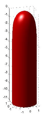
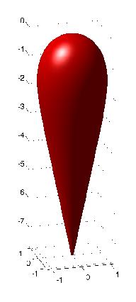
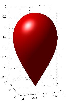
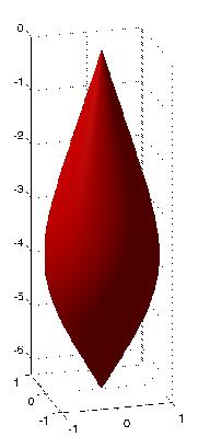
(a)	(b)	(c)	(d)

Figure 1: The deformed target spaces $(N^{\prime},\Omega)$ embedded as surfaces of revolution, in the cases (a) $U=1+\varphi_{3}$, (b) $U=(1+\varphi_{3})^{0.8}$, (c) $U=(1+\varphi_{3})^{0.5}$ and (d) $U=(1+\varphi_{3})^{0.5}(1-\varphi_{3})^{0.7}$.

Proposition 8

Let $\varphi:{\mathbb{R}}^{2}\rightarrow S^{2}$ be a solution of the model with $U(\varphi)=1+\varphi_{3}$ satisfying boundary condition (2.1). Then every connected component of the critical set of $\varphi$ is unbounded.

Proof.

By Proposition 6, $F_{\varphi}^{2}=U^{2}$ everywhere and so $\varphi$ maps the critical set $M_{\varphi}$ into $N_{0}=U^{-1}(0)$, the vacuum manifold. Assume, towards a contradiction, that $M_{\varphi}$ has a bounded connected component $M_{1}$. Then for $\epsilon>0$ sufficiently small the closed 1-manifold $\varphi_{3}^{-1}(-1+\epsilon)$ has a connected component $\Gamma\cong S^{1}$ whose interior contains $M_{1}$. Let $S$ be the interior of $\Gamma$ with $M_{1}$ removed, and consider the restriction of $\varphi$ to $S$. By Remark 2 this is an area-preserving surjective map from $S$ to $N_{\epsilon}=\{\varphi\>:\>-1<\varphi_{3}<-1+\epsilon\}$ with respect to $\Omega$. But $S$, being a bounded subset of ${\mathbb{R}}^{2}$, has finite area while $(N_{\epsilon},\Omega)$ has inifnite area, a contradiction. ∎

Nonetheless, this model does have solutions in every homotopy class. We construct them as follows. Let $\mathscr{A}:(0,\infty)\times{\mathbb{R}}\rightarrow{\mathbb{R}}^{2}$ be the diffeomorphism

$$\mathscr{A}:(x,y)\mapsto(\log x,xy).$$ (3.15)

This map is area-preserving (with respect to the Euclidean metric on both spaces). Let $\psi:{\mathbb{R}}^{2}\rightarrow S^{2}$ denote the unit lump solution constructed above, equations (3.2), (3.4). Then as remarked after Proposition 7, $\psi\circ\mathscr{A}$ satisfies the Bogomol’nyi equation on the half-space $(0,\infty)\times{\mathbb{R}}$. Clearly, $\lim_{x\rightarrow 0^{+}}\psi(\mathscr{A}(x,y))=(0,0,-1)$ for all $y$. Hence the map

$$\varphi:{\mathbb{R}}^{2}\rightarrow S^{2},\qquad\varphi(x,y)=\left\{\begin{array}[]{cc}\psi(\mathscr{A}(x,y))&x>0\\ (0,0,-1)&x\leq 0\end{array}\right.$$ (3.16)

is continuous and satisfies the Bogomol’nyi equation away from the line $x=0$. We claim that this is a genuine degree $1$ solution of the Bogomol’nyi equation, and hence, the field equation. This amounts to the claim that $\varphi$ is twice continuously differentiable everywhere.

Proposition 9

The mapping $\varphi:{\mathbb{R}}^{2}\rightarrow S^{2}$ defined in equation (3.16) is $C^{2}$.

Proof.

Clearly, $\varphi$ is smooth away from the line $x=0$, and all its derivatives vanish identically for $x<0$. So it suffices to show that

$$|\varphi_{x}|,|\varphi_{y}|,|\varphi_{xx}|,|\varphi_{xy}|,|\varphi_{yy}|$$ (3.17)

all vanish in the limit $x\rightarrow 0^{+}$, for all $y$. For $x>0$ we have that $\varphi(x,y)=\psi(X,Y)$ where $X=\log x$, $Y=xy$. Straightforward estimates using the explicit formulae (3.2),(3.4) yield that there exist constants $C,R_{*}>0$ such that for all $R=\sqrt{X^{2}+Y^{2}}\geq R_{*}$,

$$|\psi_{X}|,|\psi_{Y}| \leq CRe^{-R^{2}/4}$$

$$|\psi_{XX}|,|\psi_{XY}|,|\psi_{YY}| \leq CR^{2}e^{-R^{2}/4}.$$ (3.18)

Similarly, there exists constant $X_{*}<0$ such that for all $0<x<e^{X_{*}}$,

$$|X_{x}|,|X_{y}|,|Y_{x}|,|Y_{y}| \leq |y|+e^{-X}$$

$$|X_{xx}|,|X_{xy}|,|X_{yy}|,|Y_{xx}|,|Y_{xy}|,|Y_{yy}| \leq e^{-2X}.$$ (3.19)

Hence, by the chain rule, for all $0<x<x_{*}=\min\{e^{X_{*}},e^{-R_{*}}\}$ and all $y$

$$|\varphi_{x}| \leq CRe^{-R^{2}/4}(|y|+e^{-X})\leq C(|X|+ye^{X})e^{-X^{2}/4}(y+e^{-X})\rightarrow 0$$ (3.20)

as $x\rightarrow 0^{+}$, since then $X\rightarrow-\infty$. Hence $\lim_{x\rightarrow 0^{+}}|\varphi_{x}(x,y)|=0$ for all $y$. The same argument deals with $\varphi_{y}$.

Turning to the second derivatives, we see from the chain rule and estimates (3.18), (3.19) that for all $0<x<x_{*}$ and all $y$

$$|\varphi_{xx}| \leq C\left\{Re^{-R^{2}/4}e^{-2X}+R^{2}e^{-R^{2}/4}(y^{2}+e^{-2X})\right\}$$ (3.21)

$$\leq C(|X|+y+X^{2}+y^{2})(y^{2}+e^{-2X})e^{-X^{2}/4}\rightarrow 0$$

as $x\rightarrow 0^{+}$, since then $X\rightarrow-\infty$. Hence $\lim_{x\rightarrow 0^{+}}|\varphi_{xx}(x,y)|=0$ for all $y$. The same argument deals with $\varphi_{xy},\varphi_{yy}$. ∎

It seems likely that the mapping $\varphi$ defined in (3.16) is actually smooth everywhere, but we have not proved this. Let us henceforth denote this degree 1 $C^{2}$ map, which satisfies the Bogomol’nyi equation everywhere, $\varphi_{+}$. Note that $E(\varphi_{+})=4\pi$, the topological minimum value in its homotopy class. Since it takes exactly the vacuum value on the left half-plane, one could call this solution a semi-compacton. However, by exploiting the invariance of $E$ under area-preserving diffeomorphisms further, we can construct degree 1 energy minimizers with more tightly localized support.

Consider the map

$$\mathscr{A}^{\prime}:(0,\infty)\times(-\frac{\pi}{2},\frac{\pi}{2})\rightarrow(0,\infty)\times{\mathbb{R}},\qquad\mathscr{A}^{\prime}(x,y)=(x\cos^{2}y,\tan y).$$ (3.22)

Clearly $\mathscr{A}^{\prime}$ is an area-preserving diffeomorphism. For any $\epsilon>0$, denote by $\varphi_{+}^{\epsilon}$ the $x$-translate of $\varphi_{+}$ by $\epsilon$, that is,

$$\varphi_{+}^{\epsilon}(x,y)=\varphi_{+}(x-\epsilon,y).$$ (3.23)

The support of $\varphi_{+}^{\epsilon}$ is the half plane $x\geq\epsilon$. Denote by $S$ the infinite half-strip $S=(0,\infty)\times(-\frac{\pi}{2},\frac{\pi}{2})$, and consider the mapping

$$\varphi_{\sqsubset}:{\mathbb{R}}^{2}\rightarrow S^{2},\qquad\varphi_{\sqsubset}(x,y)=\left\{\begin{array}[]{cc}\varphi_{+}^{\epsilon}(\mathscr{A}^{\prime}(x,y))&(x,y)\in S\\ (0,0,-1)&(x,y)\notin S.\end{array}\right.$$ (3.24)

By construction, this is continuous everywhere and $C^{2}$ on the complement of $\partial S$, the boundary of the strip $S$. It also satisfies the Bogomol’nyi equation on ${\mathbb{R}}^{2}\backslash\partial S$. By construction, its support is a subset of the closure of $S$. In fact,

$$\operatorname{supp}\varphi_{\sqsubset}=\{(x,y)\>:\>x\geq\epsilon/\cos^{2}y\}\subset S.$$ (3.25)

Hence $\varphi_{\sqsubset}$ is constant on a neighbourhood of $\partial S$, and so is trivially $C^{2}$ on $\partial S$. Hence $\varphi_{\sqsubset}$ is $C^{2}$ everywhere. By construction, $E(\varphi_{\sqsubset})=4\pi$, that is, $\varphi_{\sqsubset}$ is a degree 1 energy minimizer, which we call a semi-compacton. It has a single energy density maximum located at the point $(1+\epsilon,0)$. The energy density along the line $y=0$ is

$$\mathscr{E}_{\sqsubset}(x,0)=\left\{\begin{array}[]{cc}4(x-\epsilon)^{-\log(x-\epsilon)}&x>\epsilon\\ 0&x\leq\epsilon.\end{array}\right.$$ (3.26)

So $\varphi_{\sqsubset}$ has an energy tail which decays along the strip $S$ like $x^{-\log x}$, faster than any power, but slower than exponential. The energy density of $\varphi_{\sqsubset}$ (for $\epsilon$ very small) is plotted in figure 2.

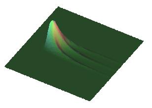
Figure 2: The energy density of a semi-compacton.

By precomposing $\varphi_{\sqsubset}$ with an area preserving diffeomorphism

$$\mathscr{A}:{\mathbb{R}}^{2}\rightarrow{\mathbb{R}}^{2},\qquad\mathscr{A}(x,y)=(\alpha x,\alpha^{-1}y)$$ (3.27)

where $\alpha>0$, we can construct semi-compactons with support in an arbitrarily thin, half infinite strip. Similarly, the strip can be deformed to follow any non-self-intersecting half infinite curve which escapes to infinity. The mapping $\bar{\varphi}_{\sqsubset}(x,y)=\varphi_{\sqsubset}(x,-y)$ is an anti-semi-compacton, of degree $-1$. By gluing together (anti-)semi-compactons with disjoint support, one obtains $C^{2}$ energy minimizers in every homotopy class. Gluing together $n_{+}>0$ semi-compactons and $n_{-}>0$ anti-semicompactons yields degree $n=n_{+}-n_{-}$ fields which, by Proposition 5, are $C^{2}$ solutions of the field equation, but have energy $4(n_{+}+n_{-})\pi>4|n|\pi$. So each homotopy class contains critical points of $E$ of arbitrarily high energy. Even more surprising, these critical points are not saddle points of $E$ but are, in a certain sense, linearly stable.

To see this, one must construct the Hessian operator for the functional $E(\varphi)$ based at a critical point $\varphi$. We recall that this is defined as follows. Let $\varphi_{s,t}$ be a two-parameter variation of a critical point $\varphi:M\rightarrow N$ of $E$, and let $X=\partial_{s}\varphi_{s,t}|_{s=t=0}$, $Y=\partial_{t}\varphi_{s,t}|_{s=t=0}\in\Gamma(\varphi^{-1}TN)$ be the associated inifnitesimal variations. Then the Hessian of $E$ at $\varphi$ is the symmetric bilinear form

$${\rm Hess}(X,Y)=\left.\frac{\partial^{2}\>}{\partial s\partial t}E(\varphi_{s,t})\right|_{s=t=0}$$ (3.28)

on $\Gamma(\varphi^{-1}TN)$. The associated Hessian operator is the self-adjoint linear differential operator $\mathscr{H}:\Gamma(\varphi^{-1}TN)\rightarrow\Gamma(\varphi^{-1}TN)$ defined such that

$${\rm Hess}(X,Y)=\int_{M}h(X,\mathscr{H}Y){\rm vol}_{M}=\langle X,\mathscr{H}Y\rangle.$$ (3.29)

One uses the spectrum of $\mathscr{H}$ to classify the critical point $\varphi$. In particular, if $\mathscr{H}$ has both negative and positive eigenvalues, $\varphi$ is a saddle point. If the quadratic form ${\rm Hess}(X,X)$ is non-negative, one says that $\varphi$ is linearly stable (although $\varphi$ may actually be dynamically unstable; e.g. $0$ is a linearly stable critical point of $f(x)=-x^{4}$).

For the energy under consideration here, one finds that [10]

$$\mathscr{H}Y=-J(\nabla^{\varphi}_{Z_{\varphi}}Y+\mathrm{d}\varphi(\sharp\delta\mathrm{d}\varphi^{*}\iota_{Y}\omega))+(\nabla^{N}_{Y}\operatorname{grad}V)\circ\varphi$$ (3.30)

where $Z_{\varphi}=\sharp\delta\varphi^{*}\omega\in\Gamma(TM)$, $\nabla^{N}$ is the Levi-Civita connexion on $TN$, $\nabla^{\varphi}$ is its pullback to $\varphi^{-1}TN$, $V=\frac{1}{2}U^{2}$ and $\iota$ denotes interior product ($\iota_{A}\omega=\omega(A,\cdot)$). The exact details of this formula are not important. We will need only the following Lemma.

Lemma 10

Let $\varphi:M\rightarrow N$ be a critical point of $E$, $\mathscr{H}$ be its Hessian operator and $x\in(M\backslash\operatorname{supp}\varphi)$. Then, for all $Y\in\Gamma(\varphi^{-1}TN)$,

$$(\mathscr{H}Y)(x)=0.$$

That is, the Hessian operator vanishes identically off the support of $\varphi$.

Proof.

The complement of $\operatorname{supp}\varphi$ is open by definition, so $\varphi$ is constant on a neighbourhood of $x$. It follows that $Z_{\varphi}=0$ and $\mathrm{d}\varphi=0$ on a neighbourhood of $x$, so the first two terms in $\mathscr{H}Y$ vanish at $x$ for all $Y$. Consider now the zeroth order piece

$$\mathscr{H}_{0}Y=(\nabla^{N}_{Y}\operatorname{grad}V)\circ\varphi.$$ (3.31)

Since $V=\frac{1}{2}U^{2}$,

$$\mathscr{H}_{0}Y=(\nabla^{N}_{Y}(U\operatorname{grad}U))\circ\varphi=(h(Y,\operatorname{grad}U)\operatorname{grad}U)\circ\varphi+(U\nabla^{N}_{Y}\operatorname{grad}U)\circ\varphi.$$ (3.32)

But $U(\varphi(x))=0$ (since $x\notin\operatorname{supp}\varphi$) and, since $U$ is assumed non-negative, $\varphi(x)$ is a minimum of $U$, and hence $(\operatorname{grad}U)(\varphi(x))=0$ also. Hence, for all $Y$, $(\mathscr{H}_{0}Y)(x)=0$ ∎

Proposition 11

Let $\varphi:M\rightarrow N$ be any solution of (2.14) constructed by superposing (anti-)
semi-compactons $\varphi_{i}$ with support in disjoint strips $S_{i}$, $i=1,2,\ldots,m$. Then for all $Y\in\Gamma^{-1}(TN)$,

$${\rm Hess}(Y,Y)\geq 0.$$

Proof.

By Lemma 10,

$${\rm Hess}(Y,Y)=\sum_{i=1}^{m}\int_{S_{i}}h(Y,\mathscr{H}_{i}Y){\rm vol}_{M}$$ (3.33)

where $\mathscr{H}_{i}$ denotes the Hessian operator associated to the (anti-)semi-compacton $\varphi_{i}$. Each term in this sum is non-negative for all $Y$. For if not, then, by Lemma 10, there exists $i$ and a section $Y$ such that

$$\langle Y,\mathscr{H}_{i}Y\rangle=\int_{M}h(Y,\mathscr{H}_{i}Y){\rm vol}_{M}=\int_{S_{i}}h(Y,\mathscr{H}_{i}Y){\rm vol}_{M}<0,$$ (3.34)

which contradicts the fact that $\varphi_{i}$ minimizes $E$ in its homotopy class. ∎

Physically, the point is that semi-compactons exert no forces on one another, so $\varphi_{\sqsubset}\bar{\varphi}_{\sqsubset}$ superpositions are (marginally) stable, by stability of their constituent parts.

So this model supports degree $n$ (marginally) stable multi-semi-compactons of energy $4(|n|+2k)\pi$ for all $n\in{\mathbb{Z}}$ and $k\in{\mathbb{Z}}_{\geq 0}$. All these solutions have (multiple) tails escaping to infinity, along which the energy density decays like $x^{-\log x}$.

4 Compactons revisited

When will an extreme baby Skyrme model support genuine compactons? The geometric picture outlined above immediately gives a necessary condition on $U$, namely that $N^{\prime}=N\backslash N_{0}$ (the target space with its vacua removed) should have finite volume with respect to the deformed area form $\Omega=\omega/U$.

Proposition 12

Let $\varphi:{\mathbb{R}}^{2}\rightarrow N$ be a surjective solution of $\tau(\varphi)=0$ of compact support. Then $(N^{\prime},\Omega)$ has finite volume.

Proof.

By Proposition 6, $F_{\varphi}^{2}=(U\circ\varphi)^{2}$ everywhere. Since $F_{\varphi}(x)=0$ if and only if $x\in M_{\varphi}$, $\varphi$ defines an area preserving map from each connected component of $M\backslash M_{\varphi}$ into $(N^{\prime},\Omega)$. The union of the ranges of each such map is all $N^{\prime}$ (since $\varphi$ is surjective), and hence the area of $N^{\prime}$ cannot exceed the area of $M\backslash M_{\varphi}\subset\operatorname{supp}\varphi$. ∎

Conversely, if $(N^{\prime},\Omega)$ has finite area $A$, let $M^{\prime}$ be any subset of $M={\mathbb{R}}^{2}$ of area $A$ which is diffeomorphic to $N^{\prime}$. For example, if $N_{0}$ consists of $p$ vacua, one could take $M^{\prime}$ to be an open disk of area $A+p\epsilon$ with $p$ small disjoint closed disks of area $\epsilon$ removed. Construct an area-preserving diffeomorphism $\psi:M^{\prime}\backslash N^{\prime}$, using the method of Moser, for example [6], and extend $\psi$ to the whole of $M$ by a piecewise constant map on $M\backslash M^{\prime}$. This map $\varphi$ certainly has compact support, and satisfies the field equation except, perhaps, on the boundary of $M^{\prime}$. Hence $\varphi$ is a genuine solution if and only if it is $C^{2}$.

For example, consider the model with

$$U(\varphi)=(1+\varphi_{3})^{\alpha}$$ (4.1)

where $\frac{1}{2}\leq\alpha<1$. Here $N^{\prime}=S^{2}\backslash\{(0,0,-1)\}$, diffeomorphic to an open disk, but, unlike the case $\alpha=1$ considered in the previous section, $N^{\prime}$ now has finite volume,

$${\rm Vol}(N^{\prime})=\int_{N^{\prime}}\frac{\omega}{U}=\int_{N^{\prime}}\frac{\mathrm{d}\Theta\wedge\mathrm{d}Z}{(1+Z)^{\alpha}}=\frac{2^{2-\alpha}}{1-\alpha}\pi.$$ (4.2)

It can be visualized as a baloon shaped surface of revolution, with a conical singularity at the missing vacuum point, see figure 1(b),(c). An obvious choice for the open set $M^{\prime}$ is the disk of radius $R=2^{1-\alpha/2}(1-\alpha)^{-\frac{1}{2}}$. There is an area-preserving diffeomorphism $M^{\prime}\rightarrow N^{\prime}$ within the radial ansatz (3.2),

$$z(r)=\left[2^{1-\alpha}-\frac{1}{2}(1-\alpha)r^{2}\right]^{\frac{1}{1-\alpha}}-1,$$ (4.3)

which, when extended by $(0,0,-1)$ outside the disk $M^{\prime}$ gives a $C^{2}$ map ${\mathbb{R}}^{2}\rightarrow S^{2}$ of degree $1$ solving the field equation everywhere. This (up to reparametrization) is the compacton reported by Adam et al [2]. Note that one can obtain its key qualitative features without solving any equations, e.g. it occupies area $\frac{2^{2-\alpha}}{1-\alpha}\pi$ and has total energy

$$E=4\pi\langle U\rangle=\frac{4\pi}{{\rm Vol}(S^{2})}\int_{S^{2}}(1+Z)^{\alpha}\mathrm{d}\Theta\wedge\mathrm{d}Z=\frac{2^{\alpha+2}}{\alpha+1}\pi.$$ (4.4)

Another interesting choice is

$$U(\varphi)=(1+\varphi_{3})^{\alpha}(1-\varphi_{3})^{\beta}$$ (4.5)

where $\alpha,\beta\in[\frac{1}{2},1)$. Now $N^{\prime}$ is diffeomorphic to a cylinder and has finite total area $A(\alpha,\beta)$, a complicated function of $\alpha,\beta$ involving hypergeometric functions. An embedding of $N^{\prime}$ as a surface of revolution in the case $\alpha=0.5$, $\beta=0.7$ is depicted in figure 1(d). One can take $M^{\prime}$ to be any annulus of total area $A$,

$$M^{\prime}=\{(x,y)\>:\>R_{1}^{2}<x^{2}+y^{2}<R_{2}^{2}\}\qquad\mbox{ where}\quad\pi(R_{2}^{2}-R_{1}^{2})=A,$$ (4.6)

and construct an area-preserving diffeomorphism $\psi:M^{\prime}\rightarrow N^{\prime}$ within the ansatz (3.2), then extend this by $(0,0,-1)$ for $r\leq R_{1}$, and $(0,0,1)$ for $r\geq R_{2}$. It is straightforward to check that this field is $C^{2}$, and hence defines a ringlike compacton. By choosing $R_{2}$ sufficiently large (and $R_{1}$ close to $R_{2}$) this ring can be arbitrarily big. Hence one can construct $n$-compactons, with $n$ rings nested inside one another, as well as the more obvious multi-ring solutions. Adam et al consider only the degenerate case that the annulus is a punctured disk [2], so we shall go through this construction in more detail.

The deformed area form (in cylindrical coordinates) is $\Omega=(1+Z)^{-\alpha}(1-Z)^{-\beta}\mathrm{d}\Theta\wedge\mathrm{d}Z$, so a field within the ansatz (3.2) satisfies the Bogomol’nyi equation if and only if

$$\frac{z^{\prime}}{(1+z)^{\alpha}(1-z)^{\beta}}=-r.$$ (4.7)

Define the function

$$Q:[-1,1]\rightarrow[0,A/(2\pi)],\qquad Q(Z)=\int_{-1}^{Z}\frac{dt}{(1+t)^{\alpha}(1-t)^{\beta}}.$$ (4.8)

Then $Q^{-1}$ is an increasing, surjective $C^{2}$ map $[0,A/(2\pi)]\rightarrow[-1,1]$, and

$$z(r)=Q^{-1}(C-\frac{r^{2}}{2})$$ (4.9)

solves (4.7) for any constant $C>0$. We require $\varphi(0,0)=(0,0,1)$, so insist that $C>A/(2\pi)$. Set $R_{1}=\sqrt{2C}$ and define $R_{2}>R_{1}$ such that $\pi(R_{2}^{2}-R_{1}^{2})=A$. Then the extended profile function is

$$z(r)=\left\{\begin{array}[]{cc}1&0\leq r\leq R_{1}\\ Q^{-1}(\frac{1}{2}(R_{1}^{2}-r^{2}))&R_{1}<r<R_{2}\\ -1&r\geq R_{2}\end{array}\right.$$ (4.10)

Note that the associated field has support in an annulus of total area $A$, as expected. Note also that it is constant in a neighbourhood of the (polar) coordinate singularity at $r=0$, so to check that $\varphi$ is $C^{2}$, it suffices to check that $z(r)$ is $C^{2}$. This is clear, except at the points $r=R_{1}$, where $z=-1$ and $r=R_{2}$, where $z=1$. By the Bogomol’nyi equation,

$$z^{\prime}(r)=-r(1+z(r))^{\alpha}(1-z(r))^{\beta}$$ (4.11)

on $(R_{1},R_{2})$, whence $\lim_{r\rightarrow R_{1}^{+}}z^{\prime}(r)=\lim_{r\rightarrow R_{2}^{-}}z^{\prime}(r)=0$. Hence $z(r)$ is $C^{1}$. Differentiating (4.11),

$$z^{\prime\prime}(r) = -(1+z(r))^{\alpha}(1-z(r))^{\beta}$$ (4.12)

$$-r^{2}\{\alpha(1+z(r))^{2\alpha-1}(1-z(r))^{2\beta}-\beta(1+z(r))^{2\alpha}(1-z(r))^{2\beta-1}\}$$

on $(R_{1},R_{2})$, whence $\lim_{r\rightarrow R_{1}^{+}}z^{\prime\prime}(r)=\lim_{r\rightarrow R_{2}^{-}}z^{\prime\prime}(r)=0$ also (note $\alpha,\beta\geq\frac{1}{2}$). Hence $z(r)$ is $C^{2}$.

One can precompose this map with an arbitrary area-preserving diffeomorphism $\mathscr{A}:{\mathbb{R}}^{2}\rightarrow{\mathbb{R}}^{2}$ to obtained deformed ring-like compactons. Choosing $R_{2}$ very close to $R_{1}$, then deforming, produces closed string-like compactons. In fact, one can precompose it with a degree $n$ area-preserving covering map

$$\mathscr{A}:{\mathbb{R}}^{2}\backslash\{(0,0)\}\rightarrow R^{2}\backslash\{(0,0)\},\qquad\mathscr{A}:(r,\theta)\mapsto(n^{-\frac{1}{2}}r,n\theta)$$ (4.13)

to obtain a degree $n$ annular compacton. Unlike the single vacuum case, this is still $C^{2}$ (even at the origin) because the degree $1$ compacton is constant on a neighbourhood of the origin.

Finally, consider the case of potential (4.5) in the case $\beta=1$. This supports a $C^{2}$ degree 1 energy minimizer which decays like $\exp(-r^{2}/2)$ to $(0,0,1)$ as $r\rightarrow\infty$, and is exactly $(0,0,-1)$ on any closed disk centred on the origin. By precomposing this with appropriate area preserving maps, as in the previous section, we can produce a semi-compacton localized in a semi-infinite strip, with a $x^{-\log x}$ tail, but with a hole (of any finite area) in the middle of the lump, where it has exactly zero energy. Clearly, by introducing more vacua, one can dream up models with even more bizarre energy minmizers.

5 Concluding remarks

We have shown that the extreme baby-Skyrme model with energy

$$E=\frac{1}{2}\int_{{\mathbb{R}}^{2}}\{[\varphi\cdot(\varphi_{x}\times\varphi_{y})]^{2}+U(\varphi)^{2}\}dx\,dy,\qquad U(\varphi)=1+\varphi_{3}$$ (5.1)

supports, in every homotopy class, semi-compacton solutions of quantized energy $E=4\pi(|n|+2k)$ where $n\in{\mathbb{Z}}$ is the degree of $\varphi$ and $k$ is a non-negative integer. These solutions are (at least) twice continuously differentiable everywhere, and consist of $|n|+2k$ (anti-)lumps, each localized in a semi-infinite strip. Each lump has a tail escaping to infinity, along which the energy density decays like $s^{-\log s}$, where $s$ is a length variable along the strip. All these solutions are at least marginally stable, and when $k=0$, are global energy minimizers in their homotopy class.

Replacing the potential term by $U=(1+\varphi_{3})^{\alpha}$, $\frac{1}{2}\leq\alpha<1$ we have given a geometric interpretation to the construction of compactons proposed in [2], and clarified the conditions under which these are $C^{2}$ (hence classical solutions of the field equation). In the case of two-vacuum potentials $U=(1+\varphi_{3})^{\alpha}(1-\varphi_{3})^{\beta}$, we have constructed annular compactons, and described how these can be embedded inside one another, and deformed into closed string-like solutions.

It is interesting to compare this situation with the case where $M$ is compact. The role of the potential term $\frac{1}{2}U^{2}$ on ${\mathbb{R}}^{2}$ is to prevent lumps dissipating by spreading indefinitely. On compact $M$, the very compactness of $M$ does this job, so one might expect that similar results (existence of minimizers in every homotopy class) might hold here in the simple case $U=0$. This turns out to be entirely false. Indeed, it was shown in [11] that all critical points of $E_{4}(\varphi)$ on a compact Riemann surface have $\varphi^{*}\omega$ coclosed. Now $\varphi^{*}\omega$ is automatically closed for all $\varphi$ (since $\mathrm{d}\varphi^{*}\omega=\varphi^{*}\mathrm{d}\omega=0$), so if $\varphi$ solves the field equation for $E_{4}$, $\varphi^{*}\omega$ is harmonic. Hence, by the Hodge Theorem, $\varphi^{*}\omega={\rm constant}\times{\rm vol}_{M}$, that is, $\varphi:M\rightarrow N$ is, up to a homothety of $(M,g)$, an area-preserving covering map, or $E_{4}(\varphi)=0$. So if the target is $N=S^{2}$, any solution either has degree $0$, or is an area-preserving diffeomorphism $M\rightarrow S^{2}$ (since $S^{2}$ is simply connected, any covering map is a diffeomorphism). It follows that if $M=S^{2}$, the model has solutions only in the degree $-1,0,1$ classes, while if $M$ is any other compact Riemann surface, it has only trivial (degree $0$, energy $0$) solutions. The contrast with $M={\mathbb{R}}^{2}$ and $U\neq 0$ is striking.

The results of this paper raise two obvious interesting questions. First, can one understand the moduli space of degree $1$ energy minimizers of this model? What about the reduced moduli space, that is, the set of minimizers modulo the action of the group of area-preserving diffeomorphisms of ${\mathbb{R}}^{2}$? Clearly, the radially symmetric lump $\psi$, the half lump $\varphi_{+}$ and the semi-compacton $\varphi_{\sqsubset}$ are three different points in this space. Do they lie in the same connected component? Is the moduli space, in fact, connected? If so, can it be given a manifold structure? If not, can its components be enumerated? Such questions are mathematically well-defined (for example, we can give the set of all maps the compact-open topology, the moduli space the relative topology from this, and the reduced moduli space the quotient topology from this) but seem formidably challenging.

Second, can one study the dynamics of semi-compactons? This question is rather subtle, because the Euler-Lagrange equation descending from the obvious Lorentz-invariant time-dependent extension of the model, with Lagrangian density

$$\mathscr{L}=\frac{1}{4}[\varphi\cdot(\partial_{\mu}\varphi\times\partial_{\nu}\varphi)][\varphi\cdot(\partial^{\mu}\varphi\times\partial^{\nu}\varphi)]-\frac{1}{2}U(\varphi)^{2}$$ (5.2)

is not a true evolution equation. The problem is that, at any spatial point $(x,y)\in{\mathbb{R}}^{2}$ where $\varphi_{x}$, $\varphi_{y}$ do not span $T_{\varphi}S^{2}$ (that is, at any critical point of $\varphi(t,\cdot):{\mathbb{R}}^{2}\rightarrow S^{2}$), the fields $\varphi$ and $\varphi_{t}$, do not uniquely determine $\varphi_{tt}$. In particular, the Cauchy problem for any initial data $\varphi(0)$, $\varphi_{t}(0)$ is ill-defined if $\varphi(0)$ has any critical points. This is immediately a problem for any initial data of degree $\geq 2$, since any such field has critical points by topological considerations. For semi-compactons, the problem is particularly severe, since these are critical on unbounded regions of ${\mathbb{R}}^{2}$. If the moduli space of semi-compactons can be understood, one could perhaps study the dynamics of a single semi-compacton within the geodesic approximation. There are some indications that the kinetic energy functional of (5.2) equips the moduli space, at least formally, with an incomplete Riemannian metric. Less speculatively, one could abandon Lorentz invariance (which is, in any case, an unnatural assumption for condensed matter applications) and give the model the usual kinetic energy term, that is,

$$\mathscr{L}=\frac{1}{2}\varphi_{t}\cdot\varphi_{t}-\frac{1}{2}[\varphi\cdot(\varphi_{x}\times\varphi_{y})]^{2}-\frac{1}{2}U(\varphi)^{2}.$$ (5.3)

The Euler-Langrange equation is now a genuine evolution equation, although it is not technically hyperbolic. It would be interesting, and numerically straightforward, to study the scattering of semi-compactons in this model.

References

[1] C. Adam, P. Klimas, J. Sánchez-Guillén and
A. Wereszczyński,
“Compact baby Skyrmions””
Phys. Rev. D80 (2009) 105013..
[2] C. Adam, T. Romanczukiewicz, J. Sánchez-Guillén and
A. Wereszczyński,
“Investigation of restricted baby Skyrme models”
Phys. Rev. D81 (2010) 085007.
[3] H. Arodź,
“Topological Compactons”
Acta Phys. PolonicaB33 (2002) 1241-1252.
[4] T. Gisiger and M.B. Paranjape,
“Solitons in a baby Skyrme model with invariance under
area-preserving diffeomorphisms”
Phys. Rev. D55 (1997) 7731-7738.
[5] J.M. Izquierdo, M.S. Rashid, B. Piette and W.J. Zakrzewski,
“Model with solitons in (2 + 1) dimensions”
Z. Phys. C53 (1992) 177-182.
[6] J. Moser,
“On the volume elements on a manifold”
Trans. Am. Math. Soc. 120 (1965) 286-294.
[7] B. Piette, D.H. Tchrakian and W.J. Zakrzewski,
“A class of two-dimensional models with extended structure solutions”
Z. Phys. C54 (1992) 497-502.
[8] P. Rosenau and J.M. Hyman,
“Compactons: solitons with finite wavelength”
Phys. Rev. Lett. 70 (1993) 564-567.
[9] M. de Innocentis and R.S. Ward,
“Skyrmions on the two sphere”
Nonlinearity14 (2001) 663-671.
[10] J.M. Speight and M. Svensson,
“On the strong coupling limit of the Faddeev-Hopf model”
Commun. Math. Phys. 272 (2007) 751-773.
[11] J.M. Speight and M. Svensson,
“Some global minimizers of a symplectic Dirichlet energy”
to appear in Quart. J. Math., arXiv:0804.4385v2.