Dirac-Kronig-Penney model for strain-engineered graphene

Abstract

Motivated by recent proposals on strain-engineering of graphene electronic circuits we calculate conductivity, shot-noise and the density of states in periodically deformed graphene. We provide the solution to the Dirac-Kronig-Penney model, which describes the phase-coherent transport in clean monolayer samples with an one-dimensional modulation of the strain and the electrostatic potentials. We compare the exact results to a qualitative band-structure analysis. We find that periodic strains induce large pseudo-gaps and suppress charge transport in the direction of strain modulation. The strain-induced minima in the gate-voltage dependence of the conductivity characterize the quality of graphene superstructures. The effect is especially strong if the variation of inter-atomic distance exceeds the value $a^{2}/\ell$, where $a$ is the lattice spacing of free graphene and $\ell$ is the period of the superlattice. A similar effect induced by a periodic electrostatic potential is weakened due to Klein tunnelling.

I Introduction

Graphene is recognized as the only two-dimensional crystal that withstands large deformations and high temperatures and is readily integrated into electronic circuits.Geim09 ; Neto09 ; Geim07 The high electron mobility and unique spectral characteristics single out graphene as a promising key element for electronic and optoelectronic applications.Meyer07 ; Bolotin08 ; Ponomarenko08 ; Lin10 ; Kim09 ; Wang08

The well-known Dirac dispersion of electronic excitations in graphene is responsible for a number of interesting analogies with relativistic quantum electrodynamics,Katsnelson07 but prevents the use of graphene in field-effect transistors due to the absence of energy band-gaps.Novoselov04 ; Novoselov05 The strain-engineering of graphene circuits has been recently suggested as a means to bypass this difficulty.Pereira2009a ; Guinea10a In the Dirac-fermion picture of graphene, the strain gradient is equivalent to the presence of a pseudo-magnetic field, which can be manipulated to induce a zero-field quantum Hall effect and a topological isolator state.Guinea10b The variation of strain may also induce substantial variation in the on-site electron energies, however, this effect is reduced by screening.Oppen09

The experimental realizations of strained graphene confirm its surprisingly high elasticity and pave the way for the development of strain-engineered graphene electronics.Bunch08 ; Kim09 Different techniques have been proposed to produce graphene samples with controlled periodical variations of strain.Bao09 ; Pletikosic09 ; Parga08 First transport measurements of graphene superstructures have been already reported.Teague09 Below we analyze the phase-coherent charge transport in periodically strained graphene samples and propose a way to characterize the quality of graphene superstructures on the basis of their transport properties.

More specifically we use the exact solution of the Dirac-Kronig-Penney model to calculate density of states, conductance, and shot noise in transport through finite size graphene samples with periodic potentials. The scattering off the metal leads is taken into account in all quantities. The position, the width, and the shape of the conductance minimum as well as the shot noise maximum associated with the periodic superstructure are analyzed in detail.

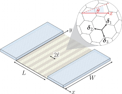
Figure 1: (Color online) Schematic illustration of the graphene setup with metal leads for $x<0$ and $x>L$. The angle $\theta$ specifies the orientation of the honeycomb lattice with respect to the transport direction $x$.

This paper is organized as follows. In Section II the effective Dirac Hamiltonian for deformed graphene is derived. The scattering approach to transport is briefly described in Section III. Section IV is devoted to the exact solution of the Dirac-Kronig-Penney model for graphene with one-dimensional modulations of strain in transport direction. The generalization of this model is discussed at the end of the Section IV. The results for conductance, shot-noise, and the density of states are qualitatively understood on the basis of the band structure analysis, which is presented in Appendix A. In Section IV.4 we discuss transport in the direction perpendicular to the strain modulation. We summarize our results in the concluding Section V.

II Effective Hamiltonian

The electromechanical coupling in deformed graphene membranes has been investigated theoretically by many authorsMorozov06 ; Guinea08 ; Kim08 ; Isacsson08 following earlier publications on carbon nanotubes.Kane97 ; Kleiner01 ; Sasaki05 ; Huertas06 The deformations affect the hopping integrals in the tight-binding description of graphene in two distinct ways: by changing the distance between carbon atoms and by tilting the electronic $p_{z}$-orbitals, which are responsible for conduction. However, for most cases of interest, the in-plane strains play the major role in determining the electronic properties of deformed graphene, while the tilting can be neglected.

The effects of in-plane strain are well captured by the tight-binding hamiltonian

$$\mathcal{H}=-\sum_{\boldsymbol{R}}\sum_{\alpha=1}^{3}\left[t+\delta t_{\alpha}(\boldsymbol{R})\right]\left(a^{\dagger}_{\boldsymbol{R}+\boldsymbol{\delta}_{\alpha}}b_{\boldsymbol{R}}+\text{h.c.}\right),$$ (1)

where the summation runs over the atomic positions, $\boldsymbol{R}$, of a honeycomb lattice, the annihilation operators $a_{\boldsymbol{R}}$ and $b_{\boldsymbol{R}}$ refer to the occupation of $p_{z}$-orbitals at the two non-equivalent positions, $A$ and $B$, of the unit cell, and the three vectors $\boldsymbol{\delta}_{\alpha}$ shown in Fig. 1 are directed from a $B$-atom to its three nearest neighbors.

If the strain varies smoothly on atomic distances, the deviation of the hopping integral from its unperturbed value $t\approx 2.7$ eV in a perfect crystal can be parameterized as

$$\delta t_{\alpha}(\boldsymbol{R})=(\beta t/a^{2})\boldsymbol{\delta}_{\alpha}^{\text{T}}\hat{u}(\boldsymbol{R})\boldsymbol{\delta}_{\alpha},$$ (2)

where $\beta=-\partial\ln t/\partial\ln a\approx 2$ and $\hat{u}(\boldsymbol{R})$ is the strain tensor of the graphene membrane.

The dimensionless strain tensor describes a change in a metric that can be expressed as

$$d\ell^{2}=d\ell_{0}^{2}+2u_{ij}ds^{i}ds^{j},$$ (3)

where the summation over the spatial indices $i,j=x,y$ is assumed. The length elements $d\ell^{2}_{0}=\delta_{ij}ds^{i}ds^{j}$ and $d\ell^{2}=g_{ij}ds^{i}ds^{j}$ correspond to the metric $\delta_{ij}$ in the flat space and to the local metric $g_{ij}$ in the membrane, respectively. In subsequent formulas we let conventionally $s^{x}=x$ and $s^{y}=y$. The graphene crystal withstands very large internal strains so that the values of the strain tensor elements may reach $20$%.Lee08

Even though the strain tensor makes no reference to the crystal structure of graphene, the lattice symmetry is entering the hopping integral in Eq. (2) due to the vectors $\boldsymbol{\delta}_{\alpha}$, $\alpha=1,2,3$. The slow variation of $\hat{u}(\boldsymbol{R})$ on the scale of the lattice spacing justifies the effective mass approximation, which is formulated in a generic reference frame shown in Fig. 1. In this frame we find

$$\boldsymbol{\delta}_{\alpha}=a\left(\begin{array}[]{c}\sin\left(\theta+\theta_{\alpha}\right)\\ -\cos\left(\theta+\theta_{\alpha}\right)\end{array}\right),\qquad\theta_{\alpha}=2\pi\alpha/3,$$ (4)

while the positions of the two non-equivalent Dirac points in the reciprocal space are given by

$$\boldsymbol{K}_{1,2}=\pm\frac{4\pi}{3a\sqrt{3}}\left(\begin{array}[]{c}\cos\theta\\ \sin\theta\end{array}\right).$$ (5)

Using the Fourier ansatz

$$a_{\boldsymbol{R}}=\sum_{s=1}^{2}e^{i\boldsymbol{K}_{s}\boldsymbol{R}}a_{s}(\boldsymbol{R}),\quad b_{\boldsymbol{R}}=\sum_{s=1}^{2}e^{i\boldsymbol{K}_{s}\boldsymbol{R}}b_{s}(\boldsymbol{R}),$$ (6)

we obtain, to the leading order in spatial gradients, the effective model

$${\cal H}=\int d^{2}\!\boldsymbol{R}\;\Psi^{\dagger}_{\boldsymbol{R}}\,\left[-i\hbar v\boldsymbol{\sigma}\boldsymbol{\nabla}+\tau_{z}\boldsymbol{\sigma}\boldsymbol{A}_{\theta}(\boldsymbol{R})\right]\,\Psi_{\boldsymbol{R}},$$ (7)

where $\hbar v=3ta/2$, $\tau_{z}$ is the Pauli matrix in the valley space and the operators are arranged into the four-spinor

$$\Psi_{\boldsymbol{R}}=\big{(}\begin{array}[]{cccc}a_{1}&e^{i\theta}b_{1}&-e^{-i\theta}b_{2}&a_{2}\end{array}\big{)}.$$ (8)

The vector field $\boldsymbol{A}_{\theta}=(A_{\theta x},A_{\theta y})$ is real and its components are related to the strain tensor in a simple way,

$$A_{\theta x}-iA_{\theta y}=(\hbar v\beta/a)e^{3i\theta}(u_{xx}+2iu_{xy}-u_{yy}).$$ (9)

In the derivation of the effective Hamiltonian (7) we neglected the velocity renormalization, which would appear as a correction of the order $\delta t_{\alpha}$ to the prefactor of the spatial gradients.deJuan07

Unlike the usual vector potential, the vector field $\boldsymbol{A}_{\theta}$ preserves the time reversal symmetry of the Hamiltonian (7). It also exhibits the discrete rotational invariance of the honeycomb lattice. Indeed, the Hamiltonian (7) remains invariant under the rotation through the angle $\theta=2\pi/3$, while the rotation through the angle $\theta=\pi/3$ is equivalent to an interchange of valleys.

The effect of a constant uniaxial strain has been studied both theoreticallyPereira2009b ; Fogler08 and experimentallyKim09 ; Mohiuddin09 and falls beyond the scope of our consideration. If the constant uniaxial strain (in $x$ direction) exceeds a certain critical value, the Dirac points merge and a band gap opens. It is predictedPereira2009b that, for a crystal expanded uniformly in the zigzag direction ($\theta=0$), the critical expansion takes on its minimal value ($\approx 23\%$), while uniaxial strain in armchair direction, $\theta=\pi/2$, never generates a gap. These predictions await experimental verification.

The strain also induces an electrostatic potential due to a change of the on-site energies of the tight-binding model. This effect leads to the appearance of a scalar electrostatic potential, which has to be added to the effective Hamiltonian (7).

III Scattering approach

In this Section we formulate the scattering approach to transport through a deformed graphene sample with metallic leads. We take advantage of the effective single-particle Hamiltonian

$$H=-i\boldsymbol{\sigma}\boldsymbol{\nabla}+\tau_{z}\boldsymbol{\sigma}\boldsymbol{A}_{\theta}+V,$$ (10)

where the fictitious vector potential $\boldsymbol{A}_{\theta}$ is related to the strain tensor, $\hat{u}(\boldsymbol{R})$, by means of the relation (9), and the scalar field $V(\boldsymbol{R})$ describes strain-induced and external electrostatic potentials. In most of the intermediate expressions we let $\hbar v=1$ for simplicity.

The metal leads are modeled by letting $V=-U_{\textrm{lead}}$ for $x<0$ and $x>L$,Tworzydlo06 in Eq. (10). The vector potential is assumed to be zero in the leads. The width of the sample in $y$ direction is denoted as $W$. The scattering off the metal leads are fully taken into account in the subsequent analysis.

The rectangular sample geometry makes it convenient to employ the Fourier transform in $y$,

$$\Psi_{\boldsymbol{R}}=\sum\limits_{q}e^{iqy}\Psi_{q}(x),$$ (11)

where $q$ is the quasiparticle momentum component parallel to the graphene-metal interface. The momentum takes on the quantized values, $q=q_{n}$, which depend on the boundary conditions in $y$ direction, for example, $q_{n}=2\pi n/W$ with integer $n$ for periodic boundary conditions. In the limit $W\gg L$, which we assume below, the particular type of the boundary conditions is not important.

We also restrict our consideration to small energies, $|\varepsilon|\ll U_{\textrm{lead}}$, where the energy $\varepsilon$ is measured with respect to the Dirac point. In this approximation we derive the equation on the transfer matrix in the formTitov07

$$\frac{\partial{\cal M}}{\partial x}=\left[\sigma_{x}(\hat{q}+\tau_{z}\hat{A}_{\theta y})+i\sigma_{z}(\hat{V}\!-\!\varepsilon)+i\tau_{z}\hat{A}_{\theta x}\right]{\cal M},$$ (12)

where we introduced matrix notation in Fourier (channel) space, e.g.

$$\hat{V}_{nm}(x)=\frac{1}{W}\int_{0}^{W}\!\!\!dy\,e^{i(q_{n}-q_{m})y}\,V(x,y),$$ (13)

and $\hat{q}_{nm}=\delta_{nm}q_{n}$. The transfer matrix has the following structure in $\sigma$-space

$${\cal M}=\begin{pmatrix}1/\hat{t}^{\prime}\phantom{}{}^{\dagger}&\hat{r}\hat{t}^{-1}\\ -\hat{t}^{-1}\hat{r}^{\prime}&1/\hat{t}\end{pmatrix},$$ (14)

where $\hat{r}$($\hat{r}^{\prime}$) for $x=L$ is the matrix of reflection amplitudes for quasiparticles entering the sample from the left(right) lead. The matrices $\hat{t}$ and $\hat{t}^{\prime}$ contain the corresponding transmission amplitudes. Then, the Landauer formula for the conductance can be cast in the following form

$$G=\frac{2e^{2}}{h}{\mathrm{Tr}}\,\hat{t}\hat{t}^{\dagger}=\frac{2e^{2}}{h}{\mathrm{Tr}}\,\left[\hat{{\cal M}}_{11}\hat{{\cal M}}_{11}^{\dagger}\right]^{-1},$$ (15)

where the trace is referred to the valley and channel space and the symbol $\hat{{\cal M}}_{11}$ stands for the $11$ block of the transfer matrix in $\sigma$-space.

The Hamiltonian (10) with vanishing electrostatic potential, $V=0$, obeys the chiral symmetry $\sigma_{z}H\sigma_{z}=-H$, which is responsible for a non-Abelian Aharonov-Casher gauge invariance at zero energy,Aharonov79

$$\Psi^{\prime}_{0}=e^{i\phi+\tau_{z}\sigma_{z}\chi}\Psi_{0}.$$ (16)

The spatially dependent phases $\phi$ and $\chi$ can be chosen in such a way that the zero-energy spectral equation $H\Psi_{0}=0$ is reduced to the Dirac equation, $-i\boldsymbol{\sigma\nabla}\Psi^{\prime}_{0}=0$, with zero vector potential. This gauge transformation can be applied in the scattering approach in order to demonstrate that the presence of arbitrary vector potential has no effect on charge transport at the Dirac point as far as the contribution from edge states can be disregarded.Schuessler09 ; Hannes10

IV 1D Dirac-Kronig-Penney model

IV.1 Transport

One-dimensional modulations of strain were realized experimentally in suspended graphene films using the remarkably large and negative thermal expansion of graphene.Bao09 Motivated by these experiments we calculate the transport properties of the one-dimensional Dirac-Kronig-Penney model, which has been introduced earlier by several authors.Masir09 ; Barbier10 ; Arovas10 Below we consider a general form of the model, where the variation of both electrostatic as well as vector potentials is included. Using the scattering approach formulated in the Section III we provide simple analytical solutions for transport and density of states in this model, which complement previous theoretical studies of Dirac Fermions in periodic potentials.Park08a ; Park08b ; DellAnna09 ; Snyman2009 ; Brey2009 ; Esmailpour10 ; Li2010 ; Tan10 ; Park2010 ; Novikov05

A graphene sample with one-dimensional modulation of strain is characterized only by the component $u_{xx}(x)$ of the strain tensor, which depends solely on the $x$-coordinate. From Eq. (9), the components of the pseudo-vector potential take the form

$$A_{\theta x}=\frac{\beta u_{xx}}{a}\cos 3\theta,\qquad A_{\theta y}=-\frac{\beta u_{xx}}{a}\sin 3\theta\,.$$ (17)

In addition, the strain induces a spatial variation of electrostatic potential, $V=V(x)$. Its relation to the strain tensor is, however, complicated by screening effects.

Since the potentials depend only on $x$, the transverse momentum $q$ is conserved. In this case the matrices $\hat{V}$, $\hat{A}_{\theta x}$ and $\hat{A}_{\theta y}$ in Eq. (12) are diagonal in channel space. Since the considered potentials also do not couple the valleys, the scattering problem is reduced to the solution of $2\times 2$ matrix equation,

$$\frac{\partial{\cal M}}{\partial x}=\left[\sigma_{x}(q+A_{\theta y})-i\sigma_{z}(\varepsilon-V)+iA_{\theta x}\right]{\cal M}.$$ (18)

The $x$-component of the vector potential, $A_{\theta x}$, enters the equation in a trivial way and can be excluded by the gauge transformation ${\cal M}\to{\cal M}\exp(i\int_{0}^{x}A_{\theta x}dx^{\prime})$, which does not affect any observable. The first and the most trivial consequence of this transformation is that the one-dimensional strain modulations in $x$ direction have no effect on transport in the zigzag direction ($\theta=2\pi n/3$ with integer $n$) provided the effect of $V$ is ignored.

For other angles the one-dimensional strain modulations lead to the appearance of new minima in the gate voltage dependence of the conductivity of the graphene sample. The numerical solution of Eq. (18) suggests that a periodic vector potential induces much more pronounced minima than a periodic scalar potential of equivalent amplitude. The weaker effect of $V$ can be associated with Klein tunnelling, which leads to the suppression of pseudo-gaps in the spectrum of the superstructure.

In order to describe the effect of periodic potentials analytically we introduce the one-dimensional Dirac-Kronig-Penney model, which is characterized by the vector potential $\boldsymbol{A}$ given by Eq. (17) with

$$u_{xx}(x)=-u_{0}/2+u_{0}\sum_{j}\Theta(x-2\ell j)\,\Theta((2j\!+\!1)\ell\!-\!x),$$ (19)

where the scale $\ell$ stands for half the period of the superlattice, $\Theta(x)$ is the Heaviside step function, and the dimensionless parameter $u_{0}$ specifies the amplitude of the strain modulation. The vector potential introduced by Eqs. (17,19) corresponds to a strain field which is smooth on atomic scale but changes abruptly on distances smaller than the Dirac quasiparticle wave length, $\hbar v/\varepsilon$. The periodic electrostatic potential is introduced in a similar manner,

$$V(x)=-V_{0}/2+V_{0}\sum_{j}\Theta(x-2\ell j)\,\Theta((2j\!+\!1)\ell\!-\!x),$$ (20)

where $V_{0}$ is the amplitude of the modulation.

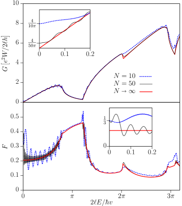
Figure 2: (Color online) Conductance and Fano factor calculated from Eq. (28) for finite systems comprising $N=10$ and $N=50$ supercells are compared with the averaged expressions to be derived in Eqs. (33,34), which correspond to the limit $N\to\infty$ and ignore contributions from evanescent modes. The plots are for graphene with strain modulations, $r_{\theta x}=1$. In a small vicinity of the Dirac point, $\varepsilon\ll\hbar v/L$, (shown at the insets) the transport is insensitive to strain due to the extended gauge invariance (16) and is dominated by the evanescent modes.

For the sake of simplicity we consider a sample of length $L=2\ell N$ with $N$ being an integer. In this case the solution to Eq. (18) satisfies ${\cal M}(L)={\cal M}_{0}^{N}$, where ${\cal M}_{0}$ is the transfer matrix corresponding to the size of the supercell, $2\ell$. Disregarding the $x$-component of the vector potential, $A_{\theta x}$, which has been argued above to have no effect on transport, we write

$${\cal M}_{0}={\cal M}_{+}{\cal M}_{-},\qquad{\cal M}_{\pm}=e^{(q_{\pm}\sigma_{x}-i\varepsilon_{\pm}\sigma_{z})\ell},$$ (21)

where we take advantage of the definitions

$$q_{\pm}=q\pm(\beta u_{0}/2a)\sin 3\theta,\qquad\varepsilon_{\pm}=\varepsilon\pm V_{0}/2.$$ (22)

The eigenvalues of the transfer matrix, ${\cal M}_{0}$, are conveniently parameterized as

$$e^{\pm 2ik_{0}\ell}=\lambda\pm i\sqrt{1-\lambda^{2}},$$ (23)

where we introduced the real function

$$\lambda=\cos k_{+}\ell\,\cos k_{-}\ell+\frac{q_{+}q_{-}\!-\!\varepsilon_{+}\varepsilon_{-}}{k_{+}k_{-}}\sin k_{+}\ell\,\sin k_{-}\ell,$$ (24)

with $k_{\pm}=(\varepsilon_{\pm}^{2}-q_{\pm}^{2})^{1/2}$ the $x$-component of the momenta. The wave number $k_{0}$ becomes imaginary for some values of $q$ and $\varepsilon$ indicating the appearance of pseudo-gaps in the superstructure. In the considered Dirac-Kronig-Penney model the value of $k_{0}$ is nothing but the $x$-component of the quasi-momentum in the reciprocal space associated with the superstructure.

In order to calculate the element ${\cal M}_{11}$ of the full transfer-matrix ${\cal M}(L)$ we use the Chebyshev identity to calculate the $N$-th power of an unimodular matrixBorn99

$${\cal M}_{0}^{N}=\frac{{\cal M}_{0}\sin k_{0}L-\sin k_{0}(L\!-\!2\ell)}{\sin 2k_{0}\ell}.$$ (25)

The matrix element $\left({\cal M}_{0}\right)_{11}=\lambda-i\eta$ is readily determined from Eqs. (21,25) with

$$\eta=\frac{\varepsilon_{-}}{k_{-}}\sin k_{-}\ell\,\cos k_{+}\ell+\frac{\varepsilon_{+}}{k_{+}}\sin k_{+}\ell\,\cos k_{-}\ell.$$ (26)

Using the fact that both $\lambda$ and $\eta$ are real functions of the energy $\varepsilon$, and the conserved momentum component $q$, we obtain from Eqs. (14,25) the exact transmission probabilities for each value of $q$,

$$T_{q}=\left[\cos^{2}{k_{0}L}+\frac{\eta^{2}}{1-\lambda^{2}}\sin^{2}{k_{0}L}\right]^{-1}.$$ (27)

This expression is reduced to the well-known result for a purely ballistic system,Tworzydlo06 i.e. for $u_{0}=V_{0}=0$, by the substitution $\eta=(\varepsilon/k)\sin 2k\ell$ and $\lambda=\cos 2k\ell$. The transmission probabilities (27) determine the energy-dependent transport quantities

$$G=\frac{4e^{2}}{h}\sum\limits_{q}T_{q},\qquad F=\frac{\sum_{q}T_{q}(1-T_{q})}{\sum_{q}T_{q}},$$ (28)

where $G$ is the Landauer conductance and $F$ is the Fano factor for the shot noise. In the limit $W\gg L$ the summation over the scattering channels can be replaced by the integration, $\sum_{q}\to(W/2\pi)\int dq$.

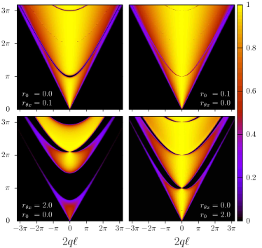
Figure 3: The density plot for the averaged transmission spectra, $\overline{T}_{q}(\varepsilon)$, calculated from Eq. (32) for the Dirac-Kronig-Penney model with strain modulation $r_{\theta x}=0.1$ (top left), $r_{\theta x}=2.0$ (bottom left) and electrostatic field modulation $r_{0}=0.1$ (top right), $r_{0}=2.0$ (bottom right).

More generally one can define the cumulant generating function for the transport,

$${\cal F}(\chi)=\sum\limits_{q}\ln(1-T_{q}+e^{\chi}T_{q}).$$ (29)

The dimensionless cumulants $c_{n}=\lim_{\chi\to 0}\partial^{n}{\cal F}/{\partial\chi^{n}}$ determine the so-called full counting statistics of the charge transport. The conductance and the Fano factor are given by $G=(4e^{2}/h)c_{1}$ and $F=c_{2}/c_{1}$, respectively.

The strength of strain-induced and electrostatic potentials in the Dirac-Kronig-Penney model (19,20) is characterized by the dimensionless parameters

$$r_{\theta x}=(2u_{0}\ell/a)\sin 3\theta,\qquad r_{0}=\ell V_{0}/\hbar v,$$ (30)

respectively. In Fig. 2 the conductance and the Fano factor in graphene with periodic modulations of strain calculated from Eq. (28) are plotted for systems with finite lengths $L=20\ell$ and $L=100\ell$ for $r_{\theta x}=1$.

The energy dependence of conductance and Fano-factor (28) reveal fast Fabry-Pérot oscillations on the scale $\hbar v/L$. From a physics point of view, these oscillations originate from multiple reflections of propagating modes (real $k_{0}$) at the metal-graphene interfaces.

The channels with imaginary values of $k_{0}$ (evanescent modes or metal-induced states) also contribute to transport. Even though the individual contribution of each evanescent mode is exponentially small, $T_{q}\sim\exp(-2L{\mathrm{Im}}\,k_{0})$, their combined effect becomes essential for energies in a vicinity of band-edges. The role of evanescent modes is especially important at the Dirac point due to the absence of propagating modes. Indeed, the conductance and the Fano-factor determined by (28) take on the values $G=4e^{2}W/\pi hL$ and $F=1/3$ for $\varepsilon\ll\hbar v/L$ irrespective of the vector potential. This universality is due to the extended gauge invariance (16).

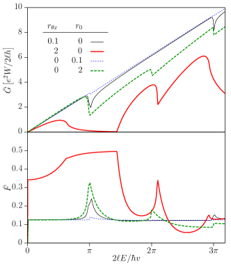
Figure 4: (Color online) The averaged conductance and Fano factor calculated from Eqs. (33,34) for the one-dimensional Dirac-Kronig-Penney model with different field strengths (30). The effect of the scalar potential is suppressed due to Klein tunnelling through potential barriers.

For $N=L/2\ell\gg 1$, the amplitude of the Fabry-Pérot oscillations in $G$ and $F$ decreases (provided $W\gg L$) and the relative contribution of evanescent modes becomes less important. Taking the limit $N\to\infty$ is equivalent to ignoring the imaginary values of $k_{0}$ and averaging over the rapid phase, $k_{0}L$. This approximation has been used e.g. in Ref. Hannes10, to obtain the full counting statistics of few-layer graphene.

The averaged generating function (29) takes the form

$$\overline{\cal F}(\chi)=2\sum\limits_{q}\ln\left(e^{\chi/2}+\sqrt{\overline{T}_{q}^{\,-2}+e^{\chi}-1}\,\right),$$ (31)

where we introduce the mean transmission probability

$$\overline{T}_{q}=|\eta|^{-1}{\mathrm{Re}}\,\sqrt{1-\lambda^{2}}.$$ (32)

The averaged transport quantities do not depend on the system size $L$ and reveal no Fabry-Pérot oscillations. For a ballistic sample, $u_{0}=V_{0}=0$, one finds $\overline{T}^{\textrm{ball}}_{q}=k/|\varepsilon|$, where $k=\sqrt{\varepsilon^{2}-q^{2}}$ is the $x$-component of the momentum.

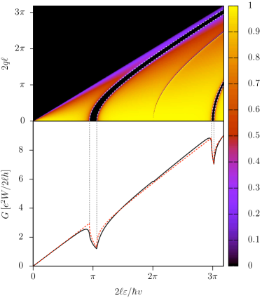
Figure 5: (Color online) The averaged conductance of Eq. (33) (solid) is compared with an estimate (35) based on the mode-counting argument (dashed) for the Dirac-Kronig-Penney model with $r_{\theta x}=0.3,r_{0}=0$. The upper panel shows the corresponding transmission spectrum.

From the generating function (31) we readily find the averaged conductance and noise. The conductance is given by the Landauer formula,

$$\overline{G}=\frac{4e^{2}}{h}\sum\limits_{q}\overline{T}_{q},$$ (33)

while the Fano-factor is related to the averaged transmission probabilities in a less evident way

$$\overline{F}=\frac{\sum_{q}\overline{T}_{q}\left(1-\overline{T}_{q}^{2}\right)}{2\sum_{q}\overline{T}_{q}}.$$ (34)

The exact and averaged transmission probabilities (27,32) together with the corresponding expressions for the full counting statistics (29,34) provide the complete analytical description of the transport properties in the 1D-Dirac-Kronig-Penney model with scalar and vector potentials of arbitrary strength.

The dependence of the transmission coefficient on the transversal momentum component, $q$, is called the transmission spectrum. In Fig. 3 we plot the transmission spectra obtained from Eq. (32) for different strengths of the scalar and vector potentials.

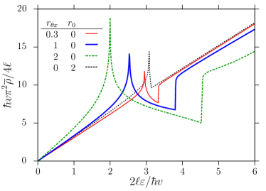
Figure 6: (Color online) The averaged density of states obtained from Eq. (43) for the Dirac-Kronig-Penney model with different strengths of the periodic potentials.

The transmission spectra shown in Fig. 3 are qualitatively different for weak, $r_{\theta x}\ll 1$, and strong, $r_{\theta x}\gg 1$, strain modulations. It has to be stressed that the latter regime is well within the experimentally accessible range of parameters. Indeed, for an achievable strain modulation of $0.2$% ($u_{0}=0.002$) and the period $\ell=70$ nm one finds $r_{\theta x}\approx 2$.

Neither the modulated strain nor the electrostatic field does open up a full band gap for any values of the parameters $r_{\theta x}$ or $r_{0}$. Nevertheless, very large pseudo-gaps are generated by strain modulations with $r_{\theta x}\gg 1$. One can see from the lower left panel in Fig. 3 that the charge transport in this regime is suppressed for almost all directions of the momenta (different $q$ values) in a wide energy range. In contrast, the pseudo-gaps do not open at normal incidence ($q=0$) in the Dirac-Kronig-Penney model with periodic electrostatic potential due to the Klein-tunnelling of quasiparticles through electrostatic barriers.Katsnelson06

The effects of strain and electrostatic field modulations on the conductance and noise are compared in Fig. 4. The most prominent feature of these plots are the dips in conductivity centered around the energies $\varepsilon_{n}=n\pi\hbar v/2\ell$ with $n=1,2,3,\dots$. The physical mechanism, which is responsible for the appearance of the pseudo-gaps, is equivalent to that of the parametric resonance.Arnold89

For $r_{\theta x}\gg 1$, the conductance is suppressed in wider energy intervals around $\varepsilon=\varepsilon_{n}$. For weak strain or potential amplitude, $r_{\theta x}\ll 1$ or $r_{0}\ll 1$, significant pseudo-gaps are only located around the energy values $\varepsilon_{n}$ with odd values of $n$, since only odd Fourier components of the potentials (19,20) exist. For a weak harmonic potential, a significant pseudo-gap would only arise around $\varepsilon=\varepsilon_{1}$.

The areas of vanishing transmission probability in Fig. 3 (top left) can be understood on the basis of perturbation theory as presented in Appendix A for small amplitudes of periodic potentials. The pseudo-gap emerging due to a weak periodic strain is described by the functions $\varepsilon_{g-}(q)$ and $\varepsilon_{g+}(q)$ given in the first row of Tab. 1. These functions are shown with dashed lines in the upper panel of Fig. 5.

Inside the pseudo-gap, i.e. for $\varepsilon_{g-}(q)<\varepsilon<\varepsilon_{g+}(q)$, the transmission coefficient is exponentially small, while it is close to the ballistic value, $\overline{T}^{\textrm{ball}}_{q}=\sqrt{\varepsilon^{2}-q^{2}}/|\varepsilon|$, outside the pseudo-gap (one can disregard the change in the resistance of the metal-graphene interface due to the weak periodic potentials). Note further, that the pseudo-gap is located near $q=0$ for energies near the dip such that $\overline{T}^{\textrm{ball}}_{q}\approx 1$ in this region. We can, therefore, estimate the conductance in the vicinity of the lowest dip ($\varepsilon=\varepsilon_{1}$) by subtracting the contribution of ballistically propagating modes inside the pseudo-gap from the ballistic result as

$$G_{mc}=G_{0}-\frac{4e^{2}}{h}\sum\limits_{q}\Theta(\varepsilon\!-\!\varepsilon_{g-}(q))\,\Theta(\varepsilon_{g+}(q)\!-\!\varepsilon),$$ (35)

where $\Theta(x)$ is the Heaviside step function, $G_{0}=e^{2}W\varepsilon/h$, and the limit $W|\varepsilon|\gg 1$ is assumed. The generalisation of Eq. (35) around the higher resonant energies, $\varepsilon=\varepsilon_{n},n=3,5,\dots$, is straightforward.

It is shown in Fig. 5 for $r_{\theta x}=0.3$ that the result of Eq. (35) agrees with the averaged conductance calculated from Eq. (33). The band-structure analysis (35,49) predicts characteristic dips in the conductance at $\varepsilon=n\pi\hbar v/2\ell,n=1,3,5\dots$ of the depth $\delta G=(8e^{2}W/h\pi)\sqrt{|A_{n}|n\pi/2\ell}$, where $A_{n}$ stands for $n$-th Fourier-component of the vector potential. For the Dirac-Kronig-Penney model one finds $A_{n}\propto 1/n$ hence the value of the conductance dip does not depend on $n$. We note that the validity of Eq. (35) is restricted to weak potentials. For $r_{\theta x},r_{0}\gtrsim 1$, the pseudo-gaps overlap and the perturbation theory of Appendix A is no longer applicable.

IV.2 Density of states

Let us now extend the solution of the Dirac-Kronig-Penney model to the density of states. For purely ballistic system with metal leads, both the local and the integrated density has been found in Ref. Titov10, using a Green’s function approach. Below we take advantage of an alternative route and relate the partial density of states in the channel $q$ to the corresponding transmission amplitude, $t_{q}$, by the well-known formulaBuettiker93

$$\nu_{q}=-\frac{1}{\pi}{\mathrm{Im}}\left[\frac{\partial\ln t_{q}}{\partial\varepsilon}\right].$$ (36)

Then, the integrated density of states per unit volume is given by

$$\rho(\varepsilon)=\frac{4}{LW}\sum\limits_{q}\nu_{q}(\varepsilon),$$ (37)

where the factor $4$ takes into account the spin and valley degeneracy.

The transmission amplitude is readily obtained from Eqs. (14,25) as

$$t_{q}=\frac{1}{\cos{k_{0}L}+i\zeta_{q}\sin{k_{0}L}},\qquad\zeta_{q}=\frac{\eta}{\sin 2k_{0}\ell},$$ (38)

where the wave-number $k_{0}$ and the real quantity $\eta$ are determined from the expressions (23) and (26), respectively. Therefore, the partial density of states can be calculated exactly as

$$\nu_{q}=\frac{L\zeta_{q}(dk_{0}/d\varepsilon)+\sin k_{0}L\,\cos k_{0}L\,(d\zeta_{q}/d\varepsilon)}{\pi\left(\cos^{2}k_{0}L+\zeta_{q}^{2}\sin^{2}k_{0}L\right)}.$$ (39)

Unlike the conductance or the shot noise (28), the density of states depends on the value of $U_{\textrm{lead}}$, because the spectrum in a vicinity of the band-edges is dominated by the metal-induced states (evanescent modes).

The metal proximity effectTitov10 can be seen already for purely ballistic system near the Dirac point. Indeed, for $u_{0}=V_{0}=0$, one finds

$$\nu^{\textrm{ball}}_{q}(\varepsilon)=\frac{L\varepsilon^{2}-(q^{2}/k)\cos kL\,\sin kL}{\pi(\varepsilon^{2}-q^{2}\cos^{2}kL)},$$ (40)

where $k=\sqrt{\varepsilon^{2}-q^{2}}$. At zero energy the ballistic result (40) is reduced to $\nu^{\textrm{ball}}_{q}(0)=\tanh{(qL)}/\pi q$. Therefore, the density of states at $\varepsilon=0$ in Eq. (37) acquires a logarithmic divergency. This divergency is regularized by the largest available transversal momentum $q_{\textrm{max}}$, which is simply equal to the Fermi-momentum in the metal lead, $q_{\textrm{max}}=U_{\textrm{lead}}/\hbar v$. Thus, the density of states in a close vicinity of the Dirac point, $\varepsilon\ll\hbar v/L$, is given by

$$\rho^{\textrm{ball}}(0)=\frac{4}{\pi^{2}\hbar vL}\ln\frac{U_{\textrm{lead}}L}{\hbar v},$$ (41)

in agreement with Ref. Titov10, . Similar logarithmic dependence of the density of states on $U_{\textrm{lead}}$ takes place in the Dirac-Kronig-Penney model for energies inside the pseudo-gaps.

In full analogy with the averaged generating function (31) we can introduce the averaged density of states, $\overline{\rho}$, which corresponds to the limit $L\to\infty$. In this limit we disregard the contribution of the metal-induced states by projecting on the real values of the momentum $k_{0}$ and average the result of Eq. (40) over the rapid phase $k_{0}L$. This procedure leads to the simple result

$$\overline{\nu}_{q}=\frac{L}{\pi}\left|\frac{d{\mathrm{Re}}\,k_{0}}{d\varepsilon}\right|,$$ (42)

hence, in the limit $W\gg L$, the mean density is given by

$$\overline{\rho}=\frac{2}{\pi^{2}}\int_{-\infty}^{\infty}\!\!\!dq\,\left|\frac{d{\mathrm{Re}}\,k_{0}}{d\varepsilon}\right|.$$ (43)

In the ballistic limit, $u_{0}=V_{0}=0$, Eq. (43) yields the density of states of the clean graphene $\overline{\rho}^{\textrm{ball}}=2|\varepsilon|/\pi\hbar^{2}v^{2}$. In Fig. 6 we plot the averaged density of states calculated from Eq. (43) for different strengths of the periodic potentials.

Figure 7: (Color online) The contour plot of the dispersion relation for the Dirac-Kronig-Penney model (19,20) with strain modulation $r_{\theta x}=0.3$ (top left), $r_{\theta x}=2.0$ (bottom left) and electrostatic field modulation $r_{0}=0.3$ (top right), $r_{0}=2.0$ (bottom right) at energy $\varepsilon=3.3\hbar v/2\ell$.

IV.3 Beyond the Dirac-Kronig-Penney model

The results of the previous subsections are readily generalized to a model with arbitrary periodic variation of strain and electrostatic potential in $x$ direction. The analysis of the model is reduced to the calculation of the transfer matrix, ${\cal M}_{0}$, which corresponds to the wave propagation over the distance $2\ell$, the period of the potential. In this generalized model, both the exact and the averaged full counting statistics as well as the density of states are still given by the expressions (29,31,39,42) with

$$\lambda=\frac{1}{2}{\mathrm{Tr}}\,{\cal M}_{0},\qquad\eta=\frac{i}{2}{\mathrm{Tr}}\,\sigma_{z}{\cal M}_{0},$$ (44)

and the $x$-component, $k_{0}$, of the quasi-momentum is related to $\lambda$ by Eq. (23). Thus, for a periodic potential of a general type, the full solution of the problem is reduced to the straightforward numerical evaluation of the functions $\lambda$ and $\eta$. Note, that the exact analytical expressions (24,26) are restricted to the Dirac-Kronig-Penney model and do not apply generally.

We have used Eqs. (44) to calculate the energy-dependent conductance for different amplitudes of the periodic strain in the harmonic potential, $u_{xx}=u_{0}\sin(\pi x/\ell)$. In this case, the higher pseudo-gaps are found to be suppressed for weak potentials $r_{\theta x},r_{0}\ll 1$ as compared to the Dirac-Kronig-Penney model. The lowest conductance minima around $\varepsilon=\varepsilon_{0}$ is essentially the same in both models. The models become even more similar with increasing potential strength. For $r_{\theta x},r_{0}\gtrsim 1$ the transmission spectra of the single-harmonic model, becomes almost equivalent to those of the Dirac-Kronig-Penney model for all energies.

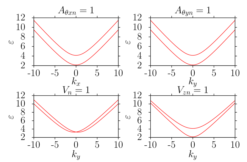
Figure 8: (Color online) Typical band gap boundaries. In all plots $n,b$ was set to 1.

IV.4 Transport in $y$ direction

We have demonstrated that periodic and $x$-dependent scalar and vector potentials modify transport in $x$-direction due to the appearance of pseudo-gaps. Let us now argue that such potentials hardly affect transport in $y$ direction, i.e. in the direction parallel to the equi-potential lines.

In Fig. 7 we plot the Fermi surface slightly above the energy value $\varepsilon=\varepsilon_{0}$ using the exact dispersion relation, $\varepsilon=\varepsilon(k_{0},q)$, obtained from Eqs. (23,24) for the Dirac-Kronig-Penney model. We have seen that the transport in $x$ direction is dominated by the modes with the momenta $q\in(-\varepsilon,\varepsilon)$. For some values of $q$ in this interval one cannot find any propagating states, which correspond to the real values of $k_{0}$. This can be seen as the formation of pseudo-gaps in the transmission spectra shown in Fig. 3, which is especially strong for $r_{\theta x},r_{0}\gtrsim 1$. In contrast, for each real value of $k_{0}$ one always finds real values of $q$. Therefore, the transport in $y$-direction is not affected by the formation of the pseudo-gaps, and depends only on the details of scattering at the metal-graphene interfaces. The latter effect is, however, weak and falls beyond the scope of our consideration. We therefore conclude that one-dimensional superlattices have a major impact only on the transport properties along the direction of their periodicity.

V Conclusion

The Dirac-Kronig-Penney model has been applied in order to study phase-coherent charge transport in periodically strained graphene samples. Using the exact relations for the band-structure in the considered superlattice, we calculate the density of states and the full counting statistics for charge transport. The exact quantities are simplified in the thermodynamic limit by neglecting the contribution of evanescent modes and averaging over the Fabry-Pérot oscillations. The conductance is found to be suppressed at energies corresponding to the positions of the pseudo-gaps in the modified spectra of the superlattice. The periodic strain and electrostatic potentials are argued to have the largest effect on transport in the direction perpendicular to the equipotential lines. The vector potentials are shown to play a greater role in confining the Dirac quasi-particles due to the suppression of Klein tunnelling.

Appendix A Band structure for Dirac particles in a superlattice

In this appendix we perturbatively calculate the band structure of a graphene sample described by the single-valley Dirac equation

$$\left[-i\boldsymbol{\sigma}\cdot\boldsymbol{\nabla}+\mathcal{V}(\boldsymbol{r})\right]\Psi(\boldsymbol{r})=\varepsilon\Psi(\boldsymbol{r}),$$ (45)

where

$$\mathcal{V}(\boldsymbol{r})=\left(\begin{array}[]{cc}V(\boldsymbol{r})+V_{z}(\boldsymbol{r})&A_{\theta x}(\boldsymbol{r})-iA_{\theta y}(\boldsymbol{r})\\ A_{\theta x}(\boldsymbol{r})+iA_{\theta y}(\boldsymbol{r})&V(\boldsymbol{r})-V_{z}(\boldsymbol{r})\end{array}\right)$$ (46)

is a general 1d-periodic potential that is smooth on the scale of the graphene lattice constant $a$. To do so, we generalize the standard methods of elementary band structure theory to the Dirac case with its non-trivial matrix structure. We find that for purely scalar potentials, this additional structure prevents the creation of a gap at $k_{y}=0$ thus making $\boldsymbol{A}_{\theta}$ and $V_{z}$ more relevant for the transport properties; this fact can be related to the chirality of the quasi-particles in graphene and the phenomenon of Klein tunnelling.

Let $\boldsymbol{b}=(b_{x},b_{y})^{\text{T}}$ span the 1d-super-lattice (so that $\mathcal{V}(\boldsymbol{r}+n\boldsymbol{b})=\mathcal{V}(\boldsymbol{r})$) and $\boldsymbol{g}$ be the corresponding reciprocal vector fixed by the conditions $\boldsymbol{g}\cdot\boldsymbol{b}=2\pi$ and $\boldsymbol{g}\parallel\boldsymbol{b}$. Making the Bloch ansatz

$$\Psi(\boldsymbol{r})=\sum_{n}\ \psi(\boldsymbol{k}-n\boldsymbol{g})\ e^{i(\boldsymbol{k}-n\boldsymbol{g})\boldsymbol{r}}$$ (47)

for the wave function and writing the periodic potential as a Fourier series, $\mathcal{V}(\boldsymbol{r})=\sum_{n}\mathcal{V}_{n}\ e^{in\boldsymbol{g}\boldsymbol{r}}$, we can write down the central equation

$$\begin{pmatrix}-\varepsilon&\mathrm{k}^{\ast}-n\mathrm{g}^{\ast}\\ \mathrm{k}-n\mathrm{g}&-\varepsilon\end{pmatrix}\psi(\boldsymbol{k}-n\boldsymbol{g})+\sum_{m}\mathcal{V}_{m-n}\psi(\boldsymbol{k}-m\boldsymbol{g})=0,$$ (48)

where $\mathrm{k}=k_{x}+ik_{y}$ and $\mathrm{g}=g_{x}+ig_{y}$. The central equation (48) represents an infinite set of linear equations for the coefficients $\psi$, which can in general only be solved numerically. The solution, however, simplifies for sufficiently weak periodic potentials.

For $\boldsymbol{k}$ close to a degeneracy, $|\boldsymbol{k}|=|\boldsymbol{k}-n\boldsymbol{g}|\approx\varepsilon$, we can neglect all but the two coefficients $\psi(\boldsymbol{k})$ and $\psi(\boldsymbol{k}-n\boldsymbol{g})$ in Eq.  (48). The resulting linear system has the simple form

$$\left|\begin{array}[]{cccc}-\varepsilon&\mathrm{k}^{*}&V+V_{z}&A_{\theta x}-iA_{\theta y}\\ \mathrm{k}&-\varepsilon&A_{\theta x}+iA_{\theta y}&V-V_{z}\\ V^{*}+V_{z}^{*}&A_{\theta x}^{*}-iA_{\theta y}^{*}&-\varepsilon&\mathrm{k}_{n}^{*}\\ A_{\theta x}^{*}+iA_{\theta y}^{*}&V^{*}-V_{z}^{*}&\mathrm{k}_{n}&-\varepsilon\end{array}\right|=0.$$ (49)

Here, we introduced the abbreviation $\mathrm{k}_{n}=\mathrm{k}-n\mathrm{g}$ and omitted the Fourier index $n$ of the potentials for brevity. The solution of Eq. (49) is particularly compact when only one of the coefficients $A_{\theta xn},A_{\theta yn},V_{n}$ or $V_{zn}$ is different from zero. In this case we obtain

$$\varepsilon^{2} = \frac{|\mathrm{k}|^{2}+|\mathrm{k}_{n}|^{2}}{2}+|U_{n}|^{2}$$ (50)

$$\pm \frac{1}{2}\sqrt{(|\mathrm{k}|^{2}-|\mathrm{k}_{n}|^{2})^{2}+4|U_{n}|^{2}|2p-n\mathrm{g}|^{2}},$$

where the pair of quantities $(U_{n},p)$ take on one of the following values $(A_{xn},k_{x})$, $(A_{yn},-ik_{y})$, $(V_{n},k)$, or $(V_{zn},0)$. We compare the energy values of the forbidden zone’s upper/lower boundary, $\varepsilon_{g\pm}$, as well as the width of the gap in forward direction for the different types of periodic potentials in Tab. 1. To calculate $\varepsilon_{g\pm}$ we have chosen $\boldsymbol{k}$ in Eq. (50) such, that $\boldsymbol{k}\cdot\boldsymbol{b}/b=n|\mathrm{g}|/2$. Typical band gap boundaries are shown in Fig. 8.

	$\varepsilon_{g\pm}$M	$\Delta(k_{y}=0)$
$A_{\theta xn}\neq 0$M	$\sqrt{k_{x}^{2}+\left|\frac{n\mathrm{g}}{2}\right|^{2}}\pm|A_{\theta xn}|$	$0$
$A_{\theta yn}\neq 0$	$\sqrt{k_{y}^{2}+\left|\frac{n\mathrm{g}}{2}\right|^{2}}\pm|A_{\theta yn}|$	$2|A_{\theta yn}|$
$V_{n}\neq 0$	$\sqrt{k_{y}^{2}+\left|\frac{n\mathrm{g}}{2}\right|^{2}+|V_{n}|^{2}\pm|k_{y}||V_{n}|}$	$0$
$V_{zn}\neq 0$	$\sqrt{k_{y}^{2}+\left|\frac{n\mathrm{g}}{2}\right|^{2}+|V_{zn}|^{2}\pm 2|\frac{n\mathrm{g}}{2}||V_{zn}|}$	$2|V_{zn}|$

Table 1: Energy value of the forbidden zone’s upper/lower boundary, as well as the width of the gap in forward direction for the different types of periodic potentials. In the first row, $\boldsymbol{b}$ was chosen parallel to $\boldsymbol{e}_{y}$, for the remaining rows $\boldsymbol{b}\parallel\boldsymbol{e}_{x}$.

References

- (1) A. Geim, Science 324, 1530 (2009).
- (2) A. H. Castro Neto, F. Guinea, N. M. R. Peres, K. S. Novoselov and A. K. Geim, Rev. Mod. Phys. 81, 109 (2009).
- (3) A. K. Geim, K. S. Novoselov, Nature Materials 6, 183 (2007).
- (4) J. C. Meyer, A. K. Geim, M. I. Katsnelson, K. S. Novoselov, T. J. Booth, and S. Roth, Nature 446, 60 (2007).
- (5) K. I. Bolotin, K. J. Sikes, J. Hone, H. L. Stormer, and P. Kim, Phys. Rev. Lett. 101, 096802 (2008).
- (6) L. A. Ponomarenko, F. Schedin, M. I. Katsnelson, R. Yang, E. W. Hill, K. S. Novoselov, and A. K. Geim, Science 320, 356 (2008).
- (7) Y.-M. Lin, C. Dimitrakopoulos, K. A. Jenkins, D. B. Farmer, H.-Y. Chiu, A. Grill, and Ph. Avouris, Science 327, 662 (2010).
- (8) K. S. Kim, Y. Z. H. Jang, S. Y. Lee, J. M. Kim, Kw. S. Kim, J.-H. Ahn, P. Kim, J.-Y. Choi, and B. H. Hong, Nature 457, 706 (2009).
- (9) X. Wang, L. Zhi, and K. Müllen, Nano Lett. 8, 323 (2008).
- (10) M. I. Katsnelson and K. S. Novoselov, Solid State Commun. 143, 3 (2007).
- (11) K. S. Novoselov, A. K. Geim, S. V. Morozov, D. Jiang, Y. Zhang, S. V. Dubonos, I. V. Grigorieva, and A. A. Firsov, Science 306, 666 (2004).
- (12) K. S. Novoselov, D. Jiang, F. Schedin, T. Booth, V. V. Khotkevich, S. V. Morozov, and A. K. Geim, PNAS 102, 10451 (2005).
- (13) V. M. Pereira and A. H. Castro Neto, Phys. Rev. Lett. 103, 046801 (2009).
- (14) F. Guinea, A. K. Geim, M. I. Katsnelson, and K. S. Novoselov, Phys. Rev. B 81, 035408 (2010).
- (15) F. Guinea, M. I. Katsnelson, and A. K. Geim, Nature Physics 6, 30 (2010).
- (16) F. von Oppen, F. Guinea, and E. Mariani, Phys. Rev. B 80, 075420 (2009).
- (17) J. Bunch, S. S. Verbridge, J. S. Alden, A. M. van der Zande, J. M. Parpia, H. G. Craighead, and P. L. McEuen, Nano Lett. 8, 2458 (2008).
- (18) W. Bao, F. Miao, Z. Chen, H. Zhang, W. Jang, C. Dames, and C. Lau, Nature Nanotechnology 4, 562 (2009).
- (19) I. Pletikosic, M. Kralj, P. Pervan, R. Brako, J. Coraux, A. T. N’Diaye, C. Busse, and T. Michely, Phys. Rev. Lett. 102, 056808 (2009).
- (20) A. L. Vazquez de Parga, F. Calleja, B. Borca, M. C. G. Passeggi, J. J. Hinarejos, F. Guinea, and R. Miranda Phys. Rev. Lett. 100, 056807 (2008) .
- (21) M. L. Teague, A. P. Lai, J. Velasco, C. R. Hughes, A. D. Beyer, M. W. Bockrath, C. N. Lau, and N.-C. Yeh, Nano Letters 9, 2542 (2009).
- (22) S. V. Morozov, K. S. Novoselov, M. I. Katsnelson, F. Schedin, L. A. Ponomarenko, D. Jiang and A. K. Geim, Phys. Rev. Lett.97, 016801 (2006).
- (23) F. Guinea, B. Horovitz and P. Le Doussal, Phys. Rev. B 77, 205421 (2008).
- (24) E. Kim, A. H. Castro Neto, Europhys. Lett. 84, 57007 (2008).
- (25) A. Isacsson, L. M Jonsson, J. M. Kinaret and M. Jonson, Phys. Rev. B 77, 035423 (2008).
- (26) C. L. Kane and E. J. Mele, Phys. Rev. Lett. 78, 1932 (1997).
- (27) A. Kleiner and S. Eggert, Phys. Rev. B 64, 113402 (2001).
- (28) K. Sasaki, Y. Kawazoe and R. Saito, Prog. Theor. Phys. 113, 463 (2005).
- (29) D. Huertas-Hernando, F. Guinea and A. Brataas, Phys. Rev. B 74, 155426 (2006).
- (30) C. Lee, X. Wei, J. W. Kysar, J. Hone, Science 321, 385 (2008).
- (31) F. de Juan, A. Cortijo, M. A. H. Vozmediano Phys. Rev. B 76, 165409 (2007).
- (32) V. M. Pereira, A. H. C. Neto, and N. M. R. Peres, Phys. Rev. B 80, 045401 (2009).
- (33) M. M. Fogler, F. Guinea, and M. I. Katsnelson, Phys. Rev. Lett. 101, 226804 (2008).
- (34) T. M. G. Mohiuddin, A. Lombardo, R. R. Nair, A. Bonetti, G. Savini, R. Jalil, N. Bonini, D. M. Basko, C. Galiotis, N. Marzari, K. S. Novoselov, A. K. Geim, and A. C. Ferrari, Phys. Rev. B, 79, 205433 (2009).
- (35) J. Tworzydlo, B. Trauzettel, M. Titov, A. Rycerz, and C. W. J. Beenakker, Phys. Rev. Lett. 96, 246802 (2006).
- (36) M. Titov, Europhys. Lett. 79, 17004 (2007).
- (37) Y. Aharonov and A. Casher, Phys. Rev. A 19, 2461 (1979).
- (38) A. Schuessler, P. M. Ostrovsky, I. V. Gornyi, and A. D. Mirlin, Phys. Rev.B 79, 075405 (2009).
- (39) W.-R. Hannes and M. Titov, Europhys. Lett. 89, 47007 (2010).
- (40) M. R. Masir, P. Vasilopoulos, F. M. Peeters, New J. Phys. 11, 095009 (2009).
- (41) M. Barbier, P. Vasilopoulos, and F. M. Peeters, Phys. Rev. B 81, 075438 (2010); Phys. Rev. B 80, 205415 (2009).
- (42) D. P. Arovas, L. Brey, H. A. Fertig, Eun-Ah Kim, K. Ziegler, arXiv:1002.3655 (2010).
- (43) C.-H. Park et al., Phys. Rev. Lett. 103, 046808 (2009); Nano Lett. 8, 2920 (2008).
- (44) C.-H. Park et al., Nature Physics 4, 213 (2008).
- (45) L. Dell’Anna and A. De Martino, Phys. Rev. B 79, 045420 (2009).
- (46) I. Snyman, Phys. Rev. B 80, 054303 (2009).
- (47) L. Brey and H. A. Fertig, Phys. Rev. Lett. 103, 046809 (2009).
- (48) M. Esmailpour, A. Esmailpour, R. Asgari, E. Elahi, and M. R. Rahimi Tabar, Solid State Commun. 150, 655 (2010).
- (49) L.-G. Wang, and S.-Y. Zhu, Phys. Rev. B 81, 205444 (2010).
- (50) L. Z. Tan, C.-H. Park, S. G. Louie, Phys. Rev. B 81, 195426 (2010).
- (51) C.-H. Park, L. Z. Tan, S. G. Louie, Physica E (2010), doi:10.1016/j.jphyse.2010.07.022
- (52) D. S. Novikov, Phys. Rev. B 72, 235428 (2005); Phys. Rev. Lett. 95, 066401 (2005).
- (53) M. Born and E. Wolf, Principles of Optics, Cambridge University Press, 1999.
- (54) M. I. Katsnelson, K. S. Novoselov, and A. K. Geim, Nature Phys. 2, 620 (2006).
- (55) V. Arnold, Mathematical methods of classical mechanics, Springer Verlag, 1989.
- (56) M. Titov, P. M. Ostrovsky, I. V. Gornyi Semicond. Sci. Technol. 25, 034007 (2010).
- (57) M. Büttiker, J. Phys.: Condensed Matter 5, 9361 (1993).