Diamond Dicing

Abstract

In OLAP, analysts often select an interesting sample of the data. For example, an analyst might focus on products bringing revenues of at least $100 000, or on shops having sales greater than $400 000. However, current systems do not allow the application of both of these thresholds simultaneously, selecting products and shops satisfying both thresholds. For such purposes, we introduce the diamond cube operator, filling a gap among existing data warehouse operations.

Because of the interaction between dimensions the computation of diamond cubes is challenging. We compare and test various algorithms on large data sets of more than 100 million facts. We find that while it is possible to implement diamonds in SQL, it is inefficient. Indeed, our custom implementation can be a hundred times faster than popular database engines (including a row-store and a column-store).

url]http://hazel-webb.com

1 Introduction

An analyst often wants to focus on an interesting part of her data set. Sometimes this means she wants to focus on only some attribute values. For example, she might select only the data related to the cities of Montreal and Toronto between the months of July and October. This operation is a dice (Section 3.1). Unfortunately, dicing requires that the analyst know

exactly which attribute values she needs. Instead of specifying the attribute values, the analyst might prefer to specify a threshold. For example, she can make an iceberg query (Section 6.3) : e.g., the cities responsible for at least $10 million in sales.

Unfortunately, it is difficult to apply thresholds over several dimensions. The analyst might have selected cities generating at least a certain volume of sales ($10 million), and then select products responsible for a certain sales volume (say $5 million) in these cities. Unfortunately, after selecting the popular products ($5 million), the constraint on cities ($10 million) may no longer be satisfied. Moreover, the analyst could equally start from a product selection that generates a sales volume of at least $5 million, and then ask which cities have sales of at least $10 million when considering only these products. This could produce a different result.

Instead, we propose diamond dicing. It applies constraints simultaneously on several dimensions in a consistent manner. For example, we may seek the cities with a sales volume of at least $10 million dollars, and products with a sales volume of at least $5 million. We require both constraints to be simultaneously satisfied. Intuitively, diamond dicing is a multidimensional generalisation of icebergs. It is also an instance of dicing, but one where the analyst need not manually specify the interesting attribute values: instead, as with an iceberg query, the analyst might only specify interesting thresholds (on sales, quantities and so on).

	Chicago	Montreal	Miami	Paris	Berlin	Totals
TV	3.4	0.9	0.1	0.9	2.0	7.3
Camcorder	0.1	1.4	3.1	2.3	2.1	9.0
Phone	0.2	6.4	2.1	3.5	0.1	12.3
Camera	0.4	2.7	5.3	4.6	3.5	16.5
Game Console	3.2	0.3	0.3	2.1	1.5	7.4
DVD Player	0.2	0.5	0.5	2.2	2.3	5.7
Totals	7.5	12.2	11.4	15.6	11.5	58.2

Figure 1: Sales (in million dollars): the shaded region is a diamond where stores in selected cities need to have sales above $10 million whereas products need sales above $5 million.

Unlike regular dicing or iceberg queries, the computation of a diamond dice (henceforth called a diamond) is a challenge because of the interaction between the dimensions. Indeed, consider Fig. 1. Applying a threshold of $10 million on sales for the cities would eliminate Chicago, whereas applying the $5-million threshold on products would not terminate any product. However, once the shops in Chicago are closed, the products TV and Game Console fall below the threshold of $5-million. We cannot stop now, after processing each dimension once: removal of these products causes the removal of the Berlin store and, finally, the termination of the DVD Player product-line. Thus, simultaneously satisfying constraints on several dimensions may require several iterations.

We must also provide guidance regarding the selection of the thresholds. In our example based on Fig. 1, we used two thresholds ($10 million for stores and $5 million for products)—but what if the analyst does not have specific thresholds in mind? As a sensible default, we might put the same threshold $k$ on both stores and products. If $k$ is too high, the diamond is empty. So we might seek $\kappa$, which is the largest value of $k$ so that the diamond is not empty. This value $\kappa$ could be an interesting default threshold for the analyst. In our example, $\kappa=7.4$ and the corresponding diamond comprises the attribute values Phone, Camera, Montreal, Miami, and Paris. Within this dice, all cities and products have at least $7.4 million in sales. We present and test efficient algorithms for finding $\kappa$ (starting in Section 3.3).

Our next section presents several motivating examples. Then we present formal definitions in Section 3. In particular, we show that our definition of a diamond is sound by proving that there is a unique solution to the diamond query. In Section 4, we present efficient algorithms to compute diamonds. We review experimentally the efficiency of our algorithms in Section 5. Finally, we review related work.

2 Motivating Examples

We consider example applications to further motivate diamond dicing. We show how diamonds allowed us to find facts that surprised us in different applications.

Bibliometrics example

Consider a bibliographic table with columns for author and venue. Perhaps we want to analyse the publication habits of professors, but much work would be required to identify precisely which authors are professors. However, perhaps we can assume that most authors without at least 5 publications, in venues where professors publish, are not professors. The diamond with a threshold of 5 publications per author and a threshold of one publication (from these authors) per venue will exclude them. This diamond is the largest author-venue subcube where authors have 5 publications each in selected venues, and where selected venues each have at least one publication from selected authors.

For illustration, we processed conference publication data available from DBLP [2]; the data and details of its preparation are given elsewhere [3]. See Table 1 for some characteristics of diamonds in this data. We find that the diamond corresponding to “professors” prunes about 82% of all authors (115 341 out of 640 674). Maybe surprisingly, it only prunes 4 venues. A similar result remains true if we compute the diamond corresponding to prolific “professors” having published at least 50 papers: out of 5 065, only 249 venues are pruned. Yet this diamond contains only 4 790 authors out of 640 674 possible authors, which is a selective group (less than 1%). Setting high thresholds is particularly useful in obtaining smaller, more easily analysed, sets of data. For these purposes, we built an interactive tool that finds the highest thresholds generating non-empty diamonds. For example, we may query for the largest value of $\kappa$ such that the following diamond  is not empty: authors with at least $\kappa$ publications each in retained venues, and retained venues each with at least $\kappa$ publications from retained authors. In this case, the answer is $\kappa=119$. We found this occurrence surprising. This diamond contains 11 prolific authors in the area of digital hardware and computer-aided design, who publish in 7 venues.

Table 1: Characteristics of selected diamonds from DBLP.

Threshold needed for each		Retained		% size
author	venue	authors	venues	reduction	interpretation
1	1	640 673	5065	0	all
5	1	115 341	5061	42	professors
50	1	4790	4816	90	prolific professors
119	119	11	7	$>$99.9	hardware cluster

In a modified form of the bibliometrics cube, we associated each publication with a main keyword, obtaining a 3-dimensional cube [4]. Putting a threshold on the keyword dimension can restrict analysis to popular or mainstream topics.

Consider constraining the authors to have at least 108 publications (on mainstream topics, in popular venues), the topics to have at least 6 occurrences (by prolific authors, in popular venues), and the venues to have at least 20 publications (by prolific authors, on mainstream topics). We find the publications of I. Pomeranz and S. M. Reddy in 8 hardware venues. Within these publications the most frequent keyword is ‘synchronous’, which occurred 7 times more often than the least frequent, ‘sequential’. Globally these keywords are almost equally frequent and are ranked 286th and 289th. These two authors are ranked 20th and 11th, globally.

Netflix example

In the Netflix movie-rating database (discussed later; see Fig. 3), users have provided ratings for various movies, and the dates of ratings are also recorded. Someone studying patterns in collaborative work might be interested that there is a subset of the Netflix data where each user entered at least 1004 ratings on movies rated at least 1004 times by these same users during days where there were at least 1004 ratings by these same users on these same movies. We found the result surprising.

Star Schema Benchmark example

We might be interested in seeking the subset of customers and suppliers such that each customer accounts for a sizable revenue with selected suppliers and the suppliers each account for a sizable revenue on those customers. We took the fact table from the Star Schema Benchmark [5] and rolled it up to two columns, customer and supplier, with revenue as the measure. (Cube SSB1 statistics are given later.) We found that about 10% of the customers (2 174) each generate revenue of at least $1.5 billion from a group of 1 996 suppliers (99.8%) and, simultaneously, each of these 1 996 suppliers generates at least $1.5 billion from the 2 174 customers. These customers and suppliers together account for approximately 17% of the total revenue and 16% of the data. Since the Star Schema Benchmark is synthetic data generated from uniform distributions [6, 7], this result is not surprising.

3 Properties of Diamond Cubes

In this section, we present a formal model of the diamond cube. We show that diamonds are nested, with a smaller diamond existing within a larger diamond. We also prove a uniqueness property for diamonds and we establish upper and lower bounds on the parameter $\kappa$ for both count and sum-based diamond cubes.

3.1 Formal Model

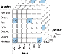
(a) 3-D cube

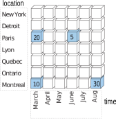
(b) Slice on product shoe

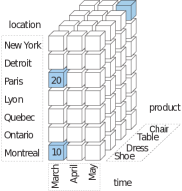
(c) Dice on months March–May

Figure 2: OLAP terms: cube, slice and dice.

Researchers and developers have yet to agree on a single multidimensional model for OLAP [8, 9] Our simplified formal model incorporates several widely accepted definitions for the terms illustrated in Fig. 2, together with new terms associated specifically with diamonds. For clarity, all terms are defined in the following paragraphs.

A dimension $D$ is a set of attributes that defines one axis of a multidimensional data structure. For example, in Fig. 2 the dimensions are location, time and product. Each dimension $D_{i}$ has a cardinality $n_{i}$, the number of distinct attribute values in this dimension. Without losing generality, we assume that $n_{1}\leq n_{2}\leq\ldots\leq n_{d}$. A dimension can be formed from a single attribute of a database relation, and the number of dimensions is denoted by $d$.

A cube is the 2-tuple ($\mathcal{D},f$) which is the set of dimensions {$D_{1},D_{2},\ldots,D_{d}$} together with a total function ($f$) which maps tuples in $D_{1}\times D_{2}\times\dots\times D_{d}$ to $\mathbb{R}\cup\{\bot\}$, where $\bot$ represents undefined. Fig. 2a shows a cube with three dimensions.

A cell of cube $C$ is a 2-tuple (($x_{1},x_{2},\ldots,x_{d})\in D_{1}\times D_{2}\times\dots\times D_{d},v$) where $v=f(x_{1},x_{2},\ldots,x_{d})$ is called a measure. The measure may be a value $v\in\mathbb{R}$, in which case we say the cell is an allocated cell. Otherwise, the measure is $\bot$ and we say the cell is empty—an unallocated cell. For the purposes of this paper, a measure is a single value. In more general OLAP applications, a cube may map to several measures. Also, measures may take values other than real-valued numbers—Booleans, for example.

A slice is the cube $C^{\prime}=(\mathcal{D}^{\prime},f^{\prime})$ obtained when a single attribute value is fixed in one dimension of cube $C=(\mathcal{D},f)$. For example, Fig. 2b is a slice of the cube presented in Fig. 2a.

A dice defines a cube $S$ from an existing cube by removing attribute values and the corresponding cells. For example, Fig. 2c illustrates a dice applied to the cube from Fig. 2a where all months except March, April and May were removed. The resulting cube still has the same number of dimensions. We call it a subcube because its dimensions are subsets of the dimensions of the original cube, and, as a function, it is a restriction to the corresponding subset of cells.

An aggregator is a function, $\sigma$, that assigns a real number to a set of cells—such as a slice. For example, sum is an aggregator: sum($\mathrm{slice}_{i}$) = $v_{1}+v_{2}+\dots+v_{m}$ where $m$ is the number of allocated cells in $\mathrm{slice}_{i}$ and the $v_{i}$’s are the measures.

A slice $S^{\prime}$ is a subset of slice $S$ if every allocated cell in $S^{\prime}$ is also an allocated cell in $S$. An aggregator $\sigma$ is monotonically non-decreasing if $S^{\prime}\subset S$ implies $\sigma(S^{\prime})\leq\sigma(S)$. Similarly, $\sigma$ is monotonically non-increasing if $S^{\prime}\subset S$ implies $\sigma(S^{\prime})\geq\sigma(S)$. Monotonically non-decreasing operators include count, max and sum over non-negative measures. Monotonically non-increasing operators include min and sum over non-positive measures. mean and median are neither monotonically non-increasing, nor non-decreasing functions.

Our formal model maps to the relational model in the following ways: (See Fig. 3.)

• A cube corresponds to a fact table: a relation whose attributes comprise a primary key and a single measure.

• An allocated cell is a fact, i.e.  it is a distinct record in a fact table.

• A dimension is one of the attributes that compose the primary key.

Movie	Reviewer	Date	Rating
1	1488844	2005-09-06	3
1	822109	2005-05-13	5
1	885013	2005-10-19	4
1	30878	2005-12-26	4
1	823519	2004-05-03	3
1	893988	2005-11-17	3
1	124105	2004-08-05	4
1	1248029	2004-04-22	3

Figure 3: Part of the NF2 fact table (see Section 5.2.1). Attributes (dimensions) are Movie, Reviewer and Date. Each row is a fact (allocated cell). The measure is Rating.

3.2 Diamond Cubes are Unique

Intuitively, a diamond cube is a subcube where all attribute values satisfy a threshold condition. For example, all selected stores must have total sales over one million dollars. We call such threshold conditions carats.

Definition 3.1.

Given a number $k$, a cube has $k$ carats along a dimension if the aggregate of every slice along that dimension is at least $k$. That is, for every slice $x$, we have $\sigma(x)\geq k$.

Note that if a dimension has $k$ carats, it necessarily has $k^{\prime}$ carats for $k^{\prime}<k$.

Given two subcubes $A$ and $B$ of the same starting cube, their union $A\cup B$ is defined by the union of the pairs of dimensions. For example, if $A$ is the result of a dice limiting the location to Montreal and $B$ is the result of a dice limiting the location to Toronto, the subcube $A\cup B$ will be the result of a dice limiting the location to both Montreal and Toronto. Similarly, the intersection ($A\cap B$) is defined by the intersection of the pairs of dimensions. We say that subcube $A$ is contained in subcube $B$ if all of the dimensions of $A$ are contained in the corresponding dimensions of $B$.

For monotonically non-decreasing operators (e.g., count, max or sum over non-negative measures), union preserves the carat, as the next proposition shows.

Proposition 3.1.

If the aggregator $\sigma$ is monotonically non-decreasing, then the union of any two cubes having $k_{i}$ (resp. $k^{\prime}_{i}$) carats along dimension $D_{i}$ has $\min(k_{i},k^{\prime}_{i})$ carats along dimension $D_{i}$ as well, for $i=\{1,2,\dots,d\}$.

Proof.

The proof follows from the monotonicity of the aggregator. ∎

If we limit ourselves to monotonically non-decreasing aggregators, then we can efficiently seek the largest possible subcube satisfying a given set of carats. We call such a subcube the diamond.

Definition 3.2.

The $k_{1},k_{2},\ldots,k_{d}$-carat diamond is the maximal subcube having
$k_{1},k_{2},\ldots,k_{d}$ carats along dimensions $D_{1},D_{2}\ldots,D_{d}$. That is, any subcube having $k_{1},k_{2},\ldots,k_{d}$ carats is contained in the diamond.

By Proposition 3.1, the diamond is unique when $\sigma$ is monotonically non-decreasing: it is given by the union of all subcubes having $k_{1},k_{2},\ldots k_{d}$ carats. For more general aggregators or when different aggregators are applied to different dimensions, the computation of the diamond might be NP-hard or ill-defined. For instance, when sum is used over cubes having both positive and negative measures, there may no longer be a unique solution to the problem ‘find the $k_{1},k_{2}\dots k_{d}$-carat cube’. This is indeed the case for the cube in Fig. 4.

row	col 1	col 2	col 3	col 4	col 5	col 6
1	-5	1	1	1	0	3
2	-3	-4	1	0	1	0
3	2	2	4	0	2	1
4	0	2	3	1	0	0

(a) Cube with positive and negative measures.

row	col 2	col 3
3	2	4
4	2	3

(b) rows processed first.

row	col 3	col 6
1	1	2
4	4	2

(c) columns processed first.

Figure 4: There is no unique 4,4-carat sum-based diamond.

Sometimes we require the same carat $k$ along all dimensions. To simplify the notation, instead of writing “$k,k,\ldots,k$-carat”, we write “$k$-carat”.

3.3 A Priori Bounds on the Carats

The computation of a diamond requires that the analyst specify the desired number of carats. However, this may not be practical for all dimensions. For example, the analyst may want to select stores with sales above one million dollars, but she may not know how to select the threshold for the product dimension. In such cases, it might be best to set the carats to the largest possible value that generates a non-empty diamond. This maximal number of carats can be found efficiently by binary search if we can determine a limited range of possible values.

Given a cube $C$ and $\sigma$, then $\kappa$ is the largest number of carats for which $C$ has a non-empty diamond. Intuitively, a small cube with many allocated cells should have a large $\kappa$, and the following proposition makes this precise.

Proposition 3.2.

For count-based carats, we have $\kappa\geq(|C|-1)/\sum_{i=1}^{d}(n_{i}-1)$.

Proof.

We begin by proving that, for count-based carats, if a cube $C$ does not contain a non-empty $k$-carat subcube, then

$$|C|\leq 1+(k-1)\sum_{i=1}^{d}(n_{i}-1).$$ (1)

Suppose that a cube $C$ of dimension at most $n_{1}\times n_{2}\times\dots\times n_{d}$ contains no $k$-carat diamond. Then one slice must contain at most $k-1$ allocated cells. Remove this slice. The amputated cube must not contain a $k$-carat diamond. Hence, it has one slice containing at most $k-1$ allocated cells. Remove it. This iterative process can continue at most $\sum_{i}(n_{i}-1)$ times before there is at most one allocated cell left: hence, there are at most $(k-1)\sum_{i}(n_{i}-1)+1$ allocated cells in total.

By definition of $\kappa$, we have that the cube does not contain a non-empty $\kappa+1$-carat subcube. By substitution ($k\rightarrow\kappa+1$) in Equation 1, we have that $|C|\leq 1+\kappa\sum_{i=1}^{d}(n_{i}-1)$. Solving for $\kappa$, we have $\kappa\geq(|C|-1)/\sum_{i=1}^{d}(n_{i}-1)$. ∎

Based on this lower bound alone, we compute $\kappa$ efficiently (see Section 5.4). For a related discussion on sum-based diamonds, see A.

4 Algorithms

Computing diamonds is challenging because of the interaction between dimensions; modifications to a measure associated with an attribute value in one dimension have a cascading effect through the other dimensions. We use different approaches to compute diamonds:

• We implemented a custom program in Java that loops through the cube checking and updating the count or sum for all attribute values in each dimension until it stabilises (see Section 4.1).

• We also implemented an algorithm using SQL (see Section 4.2).

We based both our custom and SQL implementations on the basic algorithm for computing diamonds given in Algorithm 1. Its approach is to repeatedly identify an attribute value that cannot be in the diamond, and then remove the attribute value and its slice. The identification of “bad” attribute values is done conservatively, in that they are known already to have a sum less than required ($\sigma$ is sum), or insufficient allocated cells ($\sigma$ is count). When the algorithm terminates, only attribute values that meet the condition in every slice remain: a diamond.

input : a $d-$dimensional data cube $C$, a monotonically non-decreasing aggregator $\sigma$ and $k_{1}\geq 0,k_{2}\geq 0,\ldots,k_{d}\geq 0$

output : the diamond cube $A$

$\mathtt{stable}\leftarrow\mbox{{false}}$

while $\neg\mathtt{stable}$  do

      $\mathtt{stable}\leftarrow\mbox{{true}}$

       // major iteration

       for $\mathtt{dim}=1,\ldots,d$ do

            

            for $\mathtt{i}$ in all attribute values of dimension $\mathtt{dim}$ do

                  $C_{\mathtt{dim},\mathtt{i}}\leftarrow\sigma(\text{slice }$i$\text{ on dimension }\mathtt{dim})$

                   if $C_{\mathtt{dim},\mathtt{i}}<k_{\mathtt{dim}}$ then

                        delete attribute value $\mathtt{i}$

                         if $C_{\mathtt{dim},\mathtt{i}}>0$ and $\mathtt{dim}>1$  then

                              $\mathtt{stable}\leftarrow\mbox{{false}}$

                        

return cube without deleted attribute values;

Algorithm 1 Algorithm to compute the diamond of any given cube by deleting slices eagerly.

Algorithms based on this approach always terminate, though they might sometimes return an empty cube. By specifying how to compute and maintain counts (or sums) for each attribute value in every dimension we obtain different variations. The correctness of any such variation is guaranteed by the following result.

Theorem 4.1.

Algorithm 1 is correct, that is, it always returns the $k_{1},k_{2},\ldots,k_{d}$-carat diamond.

Proof.

Because the diamond is unique, we need only show that the result of the algorithm, the cube $A$, is a diamond. If the result is not the empty cube, then dimension $D_{i}$ has at least aggregated value $k_{i}$ per slice, and hence the cube has $k_{i}$ carats. (Note that, in the main loop, if only attribute values having zero aggregates are deleted in all but the first dimension, it is not necessary to do another pass.) We only need to show that the result of Algorithm 1 is maximal: there does not exist a larger $k_{1},k_{2},\ldots,k_{d}$-carat cube.

Suppose $A^{\prime}$ is such a larger $k_{1},k_{2},\ldots,k_{d}$-carat cube. Because Algorithm 1 begins with the whole cube $C$, there must be a first time when one of the attribute values of dimension $\mathtt{dim}\textrm{ of }C$ belonging to $A^{\prime}$ but not $A$ is deleted.

At the time of deletion, the slice corresponding to this attribute value had aggregate measure less than $k_{\mathtt{dim}}$. Let $C^{\prime}$ be the cube at the instant before the attribute is deleted, with all attribute values deleted so far. We see that $C^{\prime}$ is larger than or equal to $A^{\prime}$, a $k_{1},k_{2},\ldots,k_{d}$-carat cube

and therefore, slices in $C^{\prime}$ corresponding to attribute values of $A^{\prime}$ along dimension $\mathtt{dim}$ must have aggregate measures of at least $k_{\mathtt{dim}}$, corresponding to $k_{\mathtt{dim}}$ carats Therefore, we have a contradiction and must conclude that $A^{\prime}$ does not exist and that $A$ is maximal. ∎

If the aggregator is count, and $k_{i}=1$ for $i>1$, then Algorithm 1 computes the diamond in a single pass.

4.1 Custom Software

The size of available memory affects the capacity of in-memory data structures to represent data cubes. In our experiments, we used a typical laptop computer with 8 GiB of memory. When we restricted the amount of memory available, all execution times slowed, but our custom Java software still out-performed the database management systems.

We are interested in processing large data. Therefore, we seek an efficient external memory implementation where the data cube can be stored in an external file whilst the important counts (or sums) are maintained in memory.

Algorithm 1 checks the $\sigma$-value for each attribute on every iteration. Calculating this value directly, from a data cube too large to store in main memory, would entail many expensive disk accesses. Even with the counts maintained in main memory, it is prudent to reduce the number of I/O operations as much as possible. One way this can be achieved is to store the data cube as normalised binary integers using bit compaction [10]—mapping strings to small integers starting at zero.

Algorithm 2 (External-Memory-Diamond-builder) employs $d$ arrays, $\mathtt{a}_{1}$ to $\mathtt{a}_{d}$, that map attributes to their aggregate $\sigma$-values. As values are pruned from the diamond, we must repeatedly update these arrays so that they continue to maintain the aggregate of each slice. This update can be executed in constant time for aggregators such as count and sum: in the notation of Algorithm 2, the update is computed as $\mathtt{a}_{j}(x_{j})=\mathtt{a}_{j}(x_{j})-\sigma(\{r\})$.

input : file $\mathtt{inFile}$ containing $d-$dimensional cube $C$,

integers $k_{1},k_{2},\ldots,k_{d}>0$,

monotonically non-decreasing aggregator $\sigma$,

a parameter $\tau\in[0,1)$ (we used $\tau=0.5$)

output : the cells in the diamond data cube

foreach dimension $i$ do

      Create array $\mathtt{a}_{i}$ of size $|D_{i}|$

       foreach attribute value $v$ in dimension $i$ do

            

            $\mathtt{a}_{i}(v)=\sigma($ slice for value $v$ of dimension $i$ in $C)$

$\mathtt{stable}\leftarrow\mbox{{false}}$

while $\neg\mathtt{stable}$ do

      $\mathtt{stable}\leftarrow\mbox{{true}}$

       foreach cell $r$ of $\mathtt{inFile}$ which is not marked as deleted do

            $((x_{1},x_{2},\ldots,x_{d}),v)\leftarrow r$

             for $i\in\{1,\ldots,d\}$ do

                  if $\mathtt{a}_{i}(x_{i})<k_{i}$ then

                        // attribute $x_{i}$ had previously been deleted

                         for $j\in\{1,\ldots,i-1,i+1,\ldots,d\}$  do

                              update $\mathtt{a}_{j}(x_{j})$ given the removal of cell $r$

                              

                        $\mathtt{stable}\leftarrow\mbox{{false}}$

                         mark $r$ as deleted

                         break

                        // only delete this cell once

                        

      if the fraction of cells marked as deleted exceeds $\tau$ then

            rebuild $\mathtt{inFile}$ without the deleted cells

            

rebuild $\mathtt{inFile}$ without the deleted cells

return $\mathtt{inFile}$

Algorithm 2 Diamond dicing for relationally stored cubes. With each iteration, less data is processed.

Each time the algorithm passes through the data, it updates the aggregates eagerly, and marks cells as deleted. Only when a significant fraction of the cells have been marked as such, are the cells actually deleted: we found it efficient to rebuild the list of cells when more than half have been marked as deleted ($\tau=0.5$).

When memory is abundant, we can use Algorithm 2 while keeping the content of the files in memory. Indeed, such a version was implemented and we refer to this algorithm as IMD  (In-Memory-Diamond-builder) in Section 5.

4.2 An SQL-Based Implementation

$\begin{array}[c]{|ccccccc|}\hline\cr\times&\times&&&&&\\ \times&\times&&&&&\\ &\times&\times&&&&\\ &&\times&\times&&&\\ &&&\ddots&\ddots&&\\ &&&&\times&\times&\\ &&&&&\times&\times\\ \hline\cr\end{array}$

Figure 5: An $n\times n$ cube with $2n$ allocated cells (each indicated by a $\times$) and a 2-carat diamond in the upper left: it is a difficult case for several algorithms.

Formulating a diamond cube query in SQL-92 is challenging. Using nested queries and joins, we could essentially simulate a fixed number of iterations of the outer loop in Algorithm 1. Unfortunately, we do not know how to determine the number of iterations without computing the diamond itself. Consider Fig. 5 and the corresponding 2-carat count-based diamond. Using Algorithm 1, $n-2$ iterations are required to find the diamond. That is, we see an example where the number of iterations $I=\Omega(n)$ and stopping after $o(n)$ iterations results in a poor approximation with $\Theta(n)$ allocated cells and attribute values—whereas the true 2-carat diamond has 4 attribute values and 4 allocated cells.

  INPUT: a $d-$dimensional data cube $C$ and $k>0$   OUTPUT: the diamond $A$   initialise $\mathcal{R}$ to $C$, the fact table   repeat {major iteration}      execute the fragment of SQL pseudocode shown below   until no records were deleted from $\mathcal{R}$   return $\mathcal{R}$ as $A$

⬇

CREATE TABLE $\mathit{temp}_{1}$ AS

(SELECT $\mathit{dim}_{1}$ FROM $\mathcal{R}$

GROUP BY $\mathit{dim}_{1}$ HAVING $\sigma(\mathit{measure})<k$);

$\ldots$

CREATE TABLE $\mathit{temp}_{d}$ AS

(SELECT $\mathit{dim}_{d}$ FROM $\mathcal{R}$

GROUP BY $\mathit{dim}_{d}$ HAVING $\sigma(\mathit{measure})<k$);

DELETE FROM $\mathcal{R}$

WHERE $\mathit{dim}_{1}$ IN (SELECT * FROM $\mathit{temp}_{1}$) OR $\ldots$

$\mathit{dim}_{d}$ IN (SELECT * FROM $\mathit{temp}_{d}$);

Algorithm 3 Variation where the inner two loops in Algorithm 1 are computed in SQL. This process can be repeated until $\mathcal{R}$ stabilises.

We express the essential calculation in SQL, as Algorithm 3. It is implemented as a stored procedure in SQL:1999, which allows the iterations to be controlled entirely within the DBMS. Algorithm 3 is executed against a copy of the fact table, which becomes smaller as the algorithm progresses. The fastest variation of this algorithm does not delete slices immediately, but instead updates Boolean values to indicate the slices not included in the solution. The data cube is rebuilt when 75% of the remaining cells are marked for deletion. B-tree indexes are built on each dimension to facilitate faster execution of the many GROUP BY clauses.

4.3 Complexity Analysis

Algorithm 1 visits each dimension in sequence until it stabilises. Ideally, the stabilisation should occur after as few iterations as possible.

Let $I$ be the number of iterations through the input file till convergence; i.e. no more deletions are done. Value $I$ is data dependent and (by Fig. 5) is $\Theta(\sum_{i}n_{i})$ in the worst case. In practise, $I$ is not expected to be nearly so large, and working with large real data sets $I$ did not exceed 56. Initial experiments suggested that the relationship of $I$ to $k$ would be non-decreasing to $\kappa+1$ and non-increasing thereafter. Unfortunately, there are some cubes for which this is not the case. Fig. 6 illustrates such a cube, where $\kappa=3$. On the first iteration, processing columns first for the 2-carat diamond, a single cell is deleted. On subsequent iterations at most two cells are deleted until convergence. However, the 3-carat and 4-carat diamonds converge after a single iteration.

The value of $k$ relative to $\kappa$ does, however, influence $I$. Typically, when $k$ is far from $\kappa$—either less or greater—fewer iterations are required to converge. However, when $k$ exceeds $\kappa$ by a very small amount, say 1, then typically many more iterations are required to converge to the empty cube.

$\times$	$\times$	$\times$
$\times$	$\times$	$\times$
$\times$	$\times$	$\times$
		$\times$	$\times$
		$\times$	$\times$
			$\times$	$\times$
				$\ddots$	$\ddots$
					$\times$	$\times$
						$\times$

Figure 6: The 2-carat diamond requires more iterations to converge than the 3-carat diamond. Allocated cells are indicated by a $\times$.

Algorithm 2 runs in time O($Id|C|$). Often, the number of attribute values remaining in the diamond decreases substantially in the first few iterations and those cubes are processed faster than this bound suggests. The more carats we seek, the faster the cube decreases initially.

5 Experiments

We show that diamonds can be computed efficiently, i.e. within a few minutes on a typical laptop computer, even for very large data sets. Some of the properties of diamonds, including their size and the range of values the carats may take, were assessed experimentally.

5.1 Hardware and Software

All experiments were conducted on a Gateway NV59 notebook with dual Intel i5 M430 (2.27 GHz) processors with 8 GiB of DDR3-1066 RAM running Ubuntu 12.04. The hard disk is a 596 GiB ATA WDC6400BEVT-22AORTO running at 5 400 rpm. It has an estimated reading speed of 86 MB/s.

The algorithms were implemented in Java, using SDK version 1.7.0 and the default value (1.66 GiB) for maximal heap size, and the code was archived at a public website [3]. Algorithm 3 was implemented in both an RDBMS (MySQL) and a column-store DBMS (MonetDB) [11]. RDBMS experiments were conducted on MySQL version 5.5 Community Server with MyISAM storage engine. MySQL is used in data warehousing and OLAP, most notably through vendors such as Infobright [12], JasperSoft and Pentaho [13]. The column-store experiments were conducted with MonetDB 11.11.5.

Both database implementations make use of stored procedures and a Java interface collected execution times. The drivers used were MySQL Connector/J 5.1.21 and monetdb-jdbc 2.3.

These database systems handle index creation differently:

• Of the index structures available in this version of MySQL, only B-trees are appropriate to the diamond dice operation. Spatial indexing is limited to two dimensions and hash indexing requires that the data reside in main memory. We built B-tree indexes on all columns to speed-up the GROUP-BY computations.

• In MonetDB, index creation is automatically determined with no option for the user to override system decisions [14]. Different data compression techniques, including dictionary encoding for all strings, reduce the memory footprint.

5.2 Data Used in Experiments

A varied selection of freely-available real-data sets together with some systematically generated synthetic data sets were used in the experiments. Each data set had a particular characteristic: a few dimensions or many, dimensions with high or low cardinality or a mix of the two, small or large number of cells. They were chosen to illustrate that diamond dicing is tractable under varied conditions and on many different types of data.

5.2.1 Real Data

Table 2: Statistics of data sets.

source	cube	$d$	$|C|$	$\sum_{i=1}^{d}n_{i}$	measure
King James Bible [15]	B1	4	54 601 077	31 634	count
	B2	4	24 000 000	27 042	count
	B3	4	32 000 000	29 078	count
	B4	4	40 000 000	30 417	count
	B5	4	54 601 077	31 634	sum occurrences
	B6	10	365 231 367	6 335	count
[1pt/1pt] Census Income [16]	C1	27	135 753	504	count
	C2	27	135 753	504	sum stocks
[1pt/1pt] DBLP [2]	D1	2	1 791 857	645 739	count
	D2	2	1 791 857	645 739	sum publications
	D3	3	2 516 364	689 589	count
[1pt/1pt]  Netflix [17]	NF1	3	100 478 158	484 141	count
	NF2	3	100 478 158	484 141	sum rating
	NF3	4	20 000 000	473 753	count
[1pt/1pt] Tweed [18]	TW1	4	1 957	91	count
	TW2	15	4 963	674	count
	TW3	15	4 963	674	sum killed
[1pt/1pt] Weather [19]	W1	11	124 164 371	48 654	count
	W2	11	124 164 371	48 654	sum cloud cover

Five of the real-data sets were downloaded from the following sources:

1. Census Income: http://archive.ics.uci.edu/ml [16]

2. DBLP: http://dblp.uni-trier.de/xml/

3. Netflix: http://www.netflixprize.com [17]

4. TWEED: http://folk.uib.no/sspje/tweed.htm [18]

5. Weather: http://cdiac.ornl.gov/ftp/ndp026b/ [19]

Details of how the cubes were extracted are available at a public website [3]. For cube TW1 we chose four attributes: Year, Country, Type of Action and Target of Action with cardinalities of 53, 16, 11 and 11, respectively. The attributes for cubes NF1, NF2 and NF3 are Movie (17 770), Reviewer (480 189) and Date (2 182). Rating (5) is the measure for NF2. Their statistics are given in Table 2. Each cube was stored relationally in a comma-separated file on disk. A brief description of how data cubes were extracted from the King James Bible data follows.

The data set was generated from the King James version of the Bible available at Project Gutenberg [15]. KJV-4grams [20, 21] is a data set motivated by applications of data warehousing to literature. It is a large list (with duplicates) of 4-tuples of words obtained from the verses in the King James Bible [15], after stemming with the Porter algorithm [22] and removal of stemmed words with three or fewer letters. Occurrence of row $w_{1},w_{2},w_{3},w_{4}$ indicates a verse contains words $w_{1}$ through $w_{4}$, in this order. This data is a scaled-up version of word co-occurrence cubes used to study analogies in natural language [23, 24]. These data were chosen to be representative of large cubes that might occur in text-mining applications.

Cube B1 was extracted from KJV-4grams. Duplicate records were removed and a count of each unique sequence was kept, which became the measure for cube B5. Four subcubes of B1 were also processed: B2 has the first 24 000 000 rows; B3 has the first 32 000 000 rows; and B4 has the first 40 000 000 rows. KJV-10grams has similar properties to KJV-4grams, except that there are 10 words in each row and the process of creating KJV-10grams was terminated when 500 million records had been generated—at the end of Genesis 19:30. Cube B6 was extracted from KJV-10grams. The statistics for all six cubes are also given in Table 2.

5.2.2 Synthetic Data

We took the fact table from the Star Schema Benchmark [5] and rolled-up on the supplier and customer dimensions to create cube SSB1. The result has 2 000 suppliers, 20 000 customers, and over five million rows. Uniform distributions are used to generate the benchmark [6, 7] and the data is lacking correlations between columns that real data would frequently possess.

To investigate the effect that data distribution might have on the size and shape of diamonds, nine cubes of varying dimensionality and distribution were constructed. We chose 1 000 000 cells with replacement from each of three different distributions:

• uniform—cubes U1, U2, U3.

• power law with exponent 3.5 to model the 65-35 skewed distribution—cubes S1, S2, S3.

• power law with exponent 2.0 to model the 80-20 skewed distribution—cubes SS1, SS2, SS3.

Details of the cubes generated are given in Table 3.

Table 3: Statistics of the synthetic data cubes.

Cube	$d$	$|C|$	$\sum_{i}n_{i}$	measure
SSB1	2	5 524 778	22 000	sum revenue
[1pt/1pt] U1	3	999 987	10 773	count
U2	4	1 000 000	14 364	count
U3	10	1 000 000	35 910	count
[1pt/1pt] S1	3	939 153	10 505	count
S2	4	999 647	14 296	count
S3	10	1 000 000	35 616	count
[1pt/1pt] SS1	3	997 737	74 276	count
SS2	4	999 995	99 525	count
SS3	10	1 000 000	248 703	count

5.3 Preprocessing Step

Before applying Algorithm 2, we need to convert the input (flat text files) to flat binary files. To determine if row ordering would have an effect on our implementation of Algorithm 2, we chose two cubes—C1 and B2—and shuffled the rows using the GNU utility shuf. We compared preprocessing and processing times for each of six cubes, averaged over ten runs. Extracting cubes from the data sets included a sorting step so that duplicates could be easily removed. We found that preprocessing the cube sorted on its dimension of largest cardinality was up to 25% faster than preprocessing the shuffled cube. However, execution times for Algorithm 2 were within 3% for each cube. Therefore, we did not reorder the rows prior to processing. We also found no significant difference in execution times when the cubes were sorted by different dimensions.

As stated in Section 4.1 we implemented a version (called IMD) of Algorithm 2 that reads the data cube entirely into main memory whenever the cube is small enough ($<1$ GiB). Otherwise, the algorithm processes the cube in a similar fashion.

The algorithms used in our experiments require different preprocessing of the cubes. For both Algorithms 2 and IMD, an in-memory data structure is used to maintain aggregates of the attribute values. Algorithm 3 references the cube stored in a database management system. Consequently, the preprocessor writes different kinds of data to supplementary files depending on which algorithm is to be used.

Table 4: Wall-clock times (in seconds) for preprocessing real-world data sets. A ‘—’ indicates that this algorithm was not applied to the corresponding data cube.

		3
Cube	2	MySQL	MonetDB
B1	$2.1\times 10^{2}$	$1.1\times 10^{3}$	$7.1\times 10^{1}$
B2	$5.7\times 10^{1}$	$5.0\times 10^{2}$	$3.1\times 10^{1}$
B3	$8.1\times 10^{1}$	$6.1\times 10^{2}$	$3.8\times 10^{1}$
B4	$1.6\times 10^{2}$	$7.9\times 10^{2}$	$5.3\times 10^{1}$
B6	$3.3\times 10^{3}$	—	$2.2\times 10^{3}$
C1	$2.6\times 10^{-1}$	$9.0\times 10^{0}$	$3.0\times 10^{0}$
D1	$5.0\times 10^{0}$	$1.4\times 10^{1}$	$3.7\times 10^{0}$
D3	$7.3\times 10^{0}$	$3.1\times 10^{1}$	$5.3\times 10^{0}$
NF1	$4.2\times 10^{2}$	$1.5\times 10^{3}$	$3.8\times 10^{2}$
NF3	$5.8\times 10^{1}$	$3.6\times 10^{2}$	$3.5\times 10^{1}$
W1	$1.3\times 10^{3}$	$7.4\times 10^{3}$	$1.4\times 10^{3}$

The preprocessing of the cubes was timed separately from diamond building. Preprocessed data could be used many times, varying the value for $k$, without incurring additional preparation costs. Table 4 summarises the times needed to preprocess each cube in preparation for the algorithms that were run against it. Using MonetDB was in most cases, the most efficient method. For comparison, sorting the Netflix comma-separated data file—using the GNU sort utility—took $5.3\times 10^{2}$ seconds.

5.4 Finding $\kappa$ for count-based Diamonds

Using Proposition 3.2, the $\kappa$-carat diamond was built for each of the data sets. The initial guess ($k$) for $\kappa$ was the value calculated using Proposition 3.2. Then $k$ was repeatedly doubled until an empty cube was returned and a tighter range for $\kappa$ had been established. Next a simple binary search, which used the newly discovered lower and upper bounds as the end points of the search space, was executed. Each time a non-empty diamond was returned, it was used as the input to the next iteration of the search. When the guess overshot $\kappa$ and an empty diamond was returned, the most recent non-empty cube was used as the input.

Table 5: Iterations to convergence for sum and count-based diamonds

Algorithm	cube	iterations		value of $\kappa$		time
		$\sum n_{i}$	actual	est.	actual	(in seconds)
IMD	TW1	91	6	19	38	1.0$\times 10^{-2}$
	NF3	473 753	17	39	272	6.0$\times 10^{0}$
	D1	645 739	23	3	30	3.0$\times 10^{-1}$
	D3	689 519	26	4	43	8.0$\times 10^{-1}$
	B2	27 042	16	884	7 094	5.0$\times 10^{0}$
	B3	29 078	19	1 098	8 676	6.7$\times 10^{0}$
	C1	5 607	8	282	672	1.5$\times 10^{-1}$
[1pt/1pt] EMD	NF1	484 141	19	197	1 004	3.4$\times 10^{1}$
	W1	48 654	26	2 550	4 554	6.2$\times 10^{2}$
	B1	31 634	12	1 723	14 383	1.6$\times 10^{1}$
	B4	30 417	12	1 347	10 513	1.2$\times 10^{1}$
	B6	6 335	5	57 668	112 232 566	1.0$\times 10^{3}$

(a) The number of iterations and time (in seconds) it took to determine the $\kappa$-carat diamond  for count-based diamonds.

cube	iterations		value of $\kappa$		time
	$\sum n_{i}$	actual	est.	actual	(in seconds)
B5	31 634	4	729	25 632	5.6$\times 10^{1}$
C2	504	5	1 853	3 600 675	6.0$\times 10^{-1}$
D2	645 739	7	113	119	7.5$\times 10^{-1}$
NF2	484 141	40	5	3 483	1.6$\times 10^{2}$
SSB1	22 000	8	2 124 269	1 581 756 429	4.6$\times 10^{0}$
TW3	674	3	85	85	4.3$\times 10^{-2}$
W2	48 654	19	32	20 103	1.9$\times 10^{3}$

(b) The number of iterations and time (in seconds) it took to determine the $\kappa$-carat diamond on sum-based diamonds. The estimate for $\kappa$ is the tight lower bound from Proposition A.1.

Statistics are provided in Table 5a. The estimate of $\kappa$ comes from Proposition 3.2 and the number of iterations recorded is the number used by Algorithm 2 to compute the $\kappa$-carat diamond given $\kappa$. The estimates for $\kappa$ vary between 4% and 50% of the actual value and there is no clear pattern to indicate why this might be. Two very different cubes both have estimates that are 50% of the actual value: TW1, a small cube of less than 2 000 cells and low dimensionality, and W1, a large cube of $1.23\times 10^{8}$ cells with moderate dimensionality. We experimented with sampling to provide an improved estimate for $\kappa$. We chose 10 independent samples for each of 1%, 5% and 10% using 3 of our largest cubes, which have different characteristics. We computed $\kappa$ for each of these cubes. In Table 6 we see that even with just 1% of the data, the estimate for $\kappa$ is very close to 1% of the actual value, and, therefore, provides a better estimate than that of the bound (used as an estimate) given by Proposition 3.2. Since it is an estimate, rather than a bound, we can test whether the diamond is empty for this value. Depending on the outcome, our estimate can then be used as an upper or a lower bound for the binary search.

Table 6: We can use the value of $\kappa$ from uniform samples of the data to estimate $\kappa$ for the entire cube.

Cube	Actual $\kappa$	Estimate	Sample Size (10 samples)
		from Prop 3.2	1%	1%	5%	5%	10%	10%
			min	max	min	max	min	max
NF1	1004	197	11	11	51	51	101	102
W1	4554	2550	44	45	223	224	450	451
B1	14 383	1 723	144	147	717	728	1 428	1 440

5.5 Finding $\kappa$ for sum-based Diamonds

From Proposition A.2, we have that $\min_{i}(\max_{j}(\sigma(\mathrm{slice}_{j}(D_{i}))))$ is an upper bound on $\kappa$ for any sum-based diamond  and from Proposition A.1 a lower bound is the maximum value stored in any cell. Indeed, for cube TW3  the lower bound is the $\kappa$ value. For this reason, the approach to finding $\kappa$ for the sum-based diamonds varies slightly in that the first guess for $k$ should be the lower bound + 1. If this returns a non-empty diamond, then a binary search over the range from the lower bound + 1 to the upper bound is used to find $\kappa$. Statistics are given in Table 5b.

5.6 Comparison of Algorithm Speeds

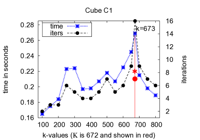
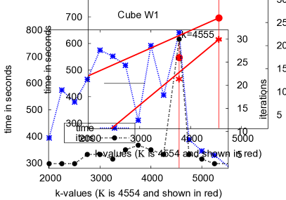
Figure 7: Times and iterations needed to generate diamonds with different $k$-values. In each case more iterations are required for $k$-values that slightly exceed $\kappa$. The increase from $k=672$ to $k=673$ is particularly evident.

In Table 5 we report times for processing the $\kappa$-carat diamond for each of nineteen cubes. Our implementation processes cubes of 20 000 000 – 40 000 000 records in less than a minute.

Table 7 compares the speeds of Algorithms 2 or IMD  with Algorithm 3. Times were averaged over five runs and then normalised against EMD or IMD. We see that EMD and IMD effect greater speed-up as the cube size increases and the cube density decreases. For example, IMD  is 4 times faster on the small, dense cube, TW1, and 2 is 500 times faster on the more sparse cube, NF3.

Although the diamond dice operation is inherently a row-wise computation, we find MonetDB can be much faster than MySQL (up to 23 times faster). MonetDB was able to complete even the most difficult computation in no more than 3.6 hours whereas MySQL needed more than 19 hours in this case. However, our Java code did it in 17 minutes. The amount of available memory affects the running times of all our algorithms. We restricted the amount of memory to 2 GiB and processed cube NF1:

• EMD was 2.6 times slower (1.5 minutes).

• MonetDB was 10 times slower (9 hours).

• MySQL was forcibly terminated after 23 hours.

Neither the initial file size nor the number of cells pruned from each $k$-carat diamond alone explains the time necessary to generate each diamond. In an earlier implementation of the diamond dicing algorithm, we had observed that the time expended was proportional to the number of cells processed. This is not as evident in the current implementation, where a new file is written when 50% of the cells are marked for deletion, instead of at every iteration. However, for all cubes more iterations and time are required to process $k$-values that only slightly exceed $\kappa$. In one instance (see Fig. 7), we need more than twice the number of iterations and nearly twice the time to compute the (empty) $k=673$-carat diamond  than to compute the $\kappa=672$-carat diamond. In both examples presented in Fig. 7 (cubes C1 and W1), the number of iterations needed to compute the $k$-carat diamond for a value of $k$ either 20% above or below $\kappa$ is at least half of the number of iterations observed for $k=\kappa+1$. Similarly, 30% more time is required to process $\kappa+1$ for cube W1. Intuitively, one should not be surprised that more iterations, and thus time, are required when $k\approx\kappa$: attribute values that are almost in the diamond are especially sensitive to other attribute values that are also almost in the diamond.

Table 7: Relative slowdown of the SQL algorithm compared to EMD or IMD. Times were averaged over ten runs. MySQL processing for cube B6 was forcibly terminated after 19 hours ($\bigotimes$).

			SQL(s)		Ratio
Cube	IMD  (s)	EMD (s)	MySQL	MonetDB	MySQL	MonetDB
C1	4.0$\times 10^{-1}$	—	1.1$\times 10^{1}$	1.0$\times 10^{1}$	2.7$\times 10^{1}$	2.5 $\times 10^{1}$
D1	3.0$\times 10^{-1}$	—	7.4$\times 10^{1}$	7.9$\times 10^{1}$	2.5$\times 10^{2}$	2.6$\times 10^{2}$
D3	8.0$\times 10^{-1}$	—	1.2$\times 10^{2}$	9.3$\times 10^{1}$	1.5$\times 10^{2}$	1.2$\times 10^{2}$
B2	—	8.0$\times 10^{0}$	1.9$\times 10^{3}$	8.2$\times 10^{1}$	2.4$\times 10^{1}$	1.0 $\times 10^{1}$
B3	—	1.2$\times 10^{1}$	2.7$\times 10^{3}$	1.1$\times 10^{2}$	2.3$\times 10^{2}$	9.0 $\times 10^{0}$
B4	—	1.2$\times 10^{1}$	3.5$\times 10^{3}$	2.2$\times 10^{2}$	2.9$\times 10^{2}$	1.8 $\times 10^{1}$
B6	—	1.0$\times 10^{3}$	$\bigotimes$	1.3$\times 10^{4}$	—	1.3 $\times 10^{1}$
NF3	6.0$\times 10^{0}$	—	1.3$\times 10^{3}$	3.3 $\times 10^{2}$	2.0$\times 10^{2}$	5.5 $\times 10^{1}$
NF1	—	3.4$\times 10^{1}$	1.9$\times 10^{4}$	5.0$\times 10^{3}$	5.6$\times 10^{2}$	1.5 $\times 10^{2}$

5.7 Diamond Size and Dimensionality

The size (in cells) of the $\kappa$-carat diamond of the high-dimensional cubes is large, e.g. the $\kappa$-carat diamond for B6 captures 30% of the data. How can we explain this? Is this property a function of the number of dimensions? To answer this question the $\kappa$-carat count-based diamond was generated for each of the synthetic cubes (except SSB1). Estimated $\kappa$, its real value and the size in cells for each cube are given in Table 8. The $\kappa$-carat diamond captures 98% of the data in cubes U1, U2 and U3—dimensionality has no effect on diamond size for these uniformly distributed data sets. Likewise, dimensionality did not affect the size of the $\kappa$-carat diamond for the skewed data cubes as it captured between 23% and 26% of the data in cubes S1, S2 and S3 and between 12% and 17% in the other cubes. These results indicate that the dimensionality of the cube does not affect how much of the data is captured by the diamond dice.

Table 8: High dimensionality does not affect diamond size.

Cube	dimensions	iters	value of $\kappa$		size (cells)	% captured
			est.	actual
U1	3	6	89	236	982 618	98
U2	4	6	66	234	975 163	98
U3	10	7	25	229	977 173	98
[1pt/1pt] S1	3	9	90	1141	227 527	24
S2	4	14	67	803	231 737	23
S3	10	14	25	208	260 864	26
[1pt/1pt] SS1	3	18	11	319	122 878	12
SS2	4	19	7	175	127 960	13
SS3	10	17	1	28	165 586	17

5.8 Iterations to Convergence

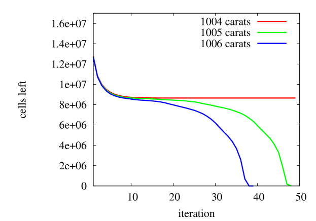
Figure 8: Cells remaining after each iteration of Algorithm 2 for $k$ = 1004, 1005 and 1006 on cube NF1.

In Section 4.3 we observed that in the worst case it could take $\Theta(\sum_{i}n_{i})$ iterations before the diamond cube stabilised. In practise this was not the case. (See Table 5 and Fig. 7). All cubes converged to the $\kappa$-carat diamond in less than 1% of $\sum_{i}n_{i}$, with the exception of the small cube TW1, which took less than 7% $\sum_{i}n_{i}$. Algorithm 2 required 19 iterations and 34 seconds to compute the 1 004-carat $\kappa$-carat diamond for NF1 and it took 50 iterations and an average of 72 seconds to determine that there is no 1 005-carat diamond.

For several values of $k$, we measured the number of cells remaining in cube NF1  after each iteration of Algorithm 2, in order to see how quickly the diamond converges to an empty diamond when $k$ exceeds $\kappa$. Fig. 8 shows the number of cells present in the diamond after each iteration for 1 004–1 006 carats. The curve for 1 006 reaches zero first, followed by that for 1 005. Since $\kappa=1\,004$, that curve stabilises at a nonzero value. It takes longer to reach a critical point when $k$ only slightly exceeds $\kappa$.

The number of iterations required until convergence for all our synthetic cubes was also far smaller than the upper bound, e.g. cube S3: 35 616 (upper bound) and 14 (actual). We had expected to see the uniformly distributed data taking longer to converge than the skewed data. This was not the case: in fact the opposite behaviour was observed. (See Table 8.) For cubes U1, U2 and U3 the diamond captured 98% of the cube: less than 23 000 cells were removed, suggesting that they started with a structure very like a diamond but for the skewed data cubes—S1, S2, S3, SS1, SS2 and SS3—the diamond was more “hidden”.

6 Related Work

There are other multidimensional operations that can be useful to an analyst, such as Skyline (Section 6.2), Nearest Neighbours and Outliers (Section 6.3). However, they differ from diamonds in several ways. Except for iterative pruning, none is a form of dicing, that is they do not select interesting attribute values, and some assume that attribute values are ordered or that we have a distance measure between records. In the rest of this section, we review these related queries in more detail.

6.1 Trawling the Web for Cyber-communities

A specialisation of the diamond cube is found in Kumar et al.’s work searching for emerging social networks on the Web [25]. Our approach is a generalisation of their two-dimensional iterative pruning algorithm. Diamonds are inherently multidimensional. Kumar et al. [25] model the Web as a directed graph and seek large dense bipartite sub-graphs. A bipartite graph is dense if most of the vertices in the two disjoint sets, $U$ and $V$, are connected. Kumar et al. hypothesise that the signature of an emerging Web community contains at least one “core”, which is a complete bipartite sub-graph with at least $i$ vertices from $U$ and $j$ vertices from $V$. In their model, the vertices in $U$ and $V$ are Web pages and the edges are links from $U$ to $V$. Seeking an ($i,j$) core is equivalent to seeking a perfect two-dimensional diamond cube (all cells are allocated). Their iterative pruning algorithm is a specialisation of the basic algorithm we use to seek diamonds: it is restricted to two dimensions and is used as a preprocessing step to prune data that cannot be included in the ($i,j$) cores. A multidimensional extension of their algorithm proved to consume too much memory and run too slowly. See [26].

6.2 Skyline Operator

The Skyline operator [27, 28] seeks a set of points where each point is not “dominated” by some others: a point is included in the skyline if it is as good or better in all dimensions and better in at least one dimension. Attributes, e.g. distance or cost, must be ordered.

Skyline queries have been adapted to the OLAP context [29] as the Multi-Objective OLAP (MOOLAP) framework. Like diamonds, the goal is to allow an analyst to focus on interesting data. For example, the analyst might be interested in stores that have either high profitability or high volume of sales (ideally both). Like diamonds, MOOLAP assumes that user-provided aggregators are monotone (e.g., like sum). In contrast to diamonds, MOOLAP results do not form a dice.

6.3 Sub-sampling with Database Queries

Relational Database Management Systems (RDBMS) have optimisation routines that are especially tuned to address both basic and more complex SELECT …FROM …WHERE … queries. However, there are some classes of queries that are difficult to express in SQL, or that execute slowly, because suitable algorithms are not available to the underlying query engine. Besides skyline, they include top-$k$ and nearest-neighbour queries.

Top-$k$

Another query, closely related to the skyline query, is that of finding the “top-$k$” data points. For example, we may seek the ten most popular products sold in a store. While this can help the work of the analyst, browsing only the top-$k$ results can also improve performance [30] by reducing the size of the result set.

Nearest Neighbours

One of the most common multidimensional queries is the nearest neighbour query, which seeks elements that are “close” to a provided target. For example, given a set of users, we might seek users who have a profile similar to the current user. A common query asks to find the $k$ nearest neighbours (kNN), that is, $k$ neighbours that are as close as possible to the target.

Reverse nearest neighbours [31] starts with a given element and asks which possible targets would have this element in the nearest neighbours. For example, imagine that customers only visit one of the 10 nearest stores. Given a customer, which store locations would attract him? Nearest neighbour queries require a specific distance measure.

Outlier Identification

Another frequent type of query in multidimensional data analysis is outlier identification. For example, we might seek elements that are far from most other data points [32]. Sarawagi et al. [33] define outliers in the OLAP context as deviations from anticipated values (computed from a model). Their approach requires learning a model from the data so that anticipated values can be computed. It also serves to highlight possibly interesting data in a large data cube.

Iceberg Queries

The iceberg query introduced by Fang et al. [34] eliminates aggregate values below some specified threshold. For example, if we have sales data by month and by store, we might require sales to exceed a threshold: only pairs (month, store) above the threshold are kept. These might be considered interesting by the analyst. In contrast, diamond dicing applies several thresholds simultaneously. In effect, we could consider diamond dicing as the simultaneous application of several interacting iceberg thresholds.

6.4 Formal Concept Analysis

In Formal Concept Analysis [35, 36] a Galois (concept) lattice is built from a binary relation. It is used in machine learning to identify conceptual structures among data sets. For example, a concept can be formed from a set of documents and the set of search terms those documents match. We put a value of 1 in a cell if the corresponding document contains the corresponding term, otherwise we leave the cell unallocated. A Galois concept in this case would be a list of documents and a list of terms such that every document contains every term in the list, and every term is contained in every document. Just like a diamond, Galois concepts must be maximal: there cannot be another Galois concept that contains all the documents and terms, and some more. Given the data in Fig. 9a, the smallest concept including document 1 is the one with documents {1, 2} and search terms {A,B,C,D}. Concepts can be partially ordered by inclusion and thus can be represented by a lattice as in Fig. 9b

Galois lattices are related to diamond cubes: in effect, a Galois concept is a perfect count-based diamond— one with all cells allocated — in a two-dimensional setting. Though formal Concept Analysis is typically restricted to two dimensions, Cerf et al. [37] generalise formal concepts by presenting an algorithm that is applied to more than two dimensions. Their definition of a closed $n-$set—a formal concept in more than two dimensions—states that each element is related to all others in the set and no other element can be added to this set without breaking the first condition. It is the equivalent of finding a perfect diamond in $n$ dimensions.

In real data sets, we are unlikely to find large perfect diamonds though we can find many small ones, especially if there are many dimensions. Galois concepts are brittle: a single omitted cell is sufficient to make a concept disappear. Thus, for an analyst, Galois concepts may be difficult to use.

Table 9: A 3-dimensional relation with closed 3-set {($\alpha,\gamma)(1,2)(A,B)$}.

		dimension 3			dimension 3			dimension 3
		A	B	C	A	B	C	A	B	C
dimension 2	1	1	1	1	1	1	1	1	1
	2	1	1		1	1		1	1
	3		1				1	1		1
	4			1	1		1	1	1	1
		$\alpha$			$\beta$			$\gamma$
		dimension 1

		Search Terms
		A	B	C	D	E
Documents	1	1	1	1	1
	2	1	1	1	1
	3	1	1	1		1
	4	1		1
	5		1	1		1

(a) A $3\times 3$ diamond is embedded in this binary relation.

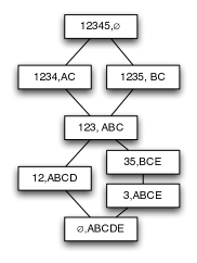
(b) Galois lattice. Each element (concept) in the lattice is defined by its extent and intent.

Figure 9: Documents and search terms in an information retrieval system and the corresponding Galois lattice.

7 Conclusion

We presented a formal analysis of the diamond cube. We have shown that, for the parameter $k$ associated with each dimension in every data cube, there is only one $k_{1},k_{2},\ldots k_{d}$-carat diamond. By varying the $k_{i}$’s we get a collection of diamonds for a cube. We established upper and lower bounds on the parameter $\kappa$ for both count and sum-based diamond cubes.

We have designed, implemented and tested algorithms to compute diamonds on real and synthetic data sets. Experimentally, the algorithms bear out our theoretical results. An unexpected experimental result is that the number of iterations required to process the diamonds with $k$ slightly greater than $\kappa$ is often twice that required to process the $\kappa$-carat diamond. This also results in an increase in running time.

We have shown that computing diamonds for large data sets is feasible. 2 fared better on large, sparse data cubes than other approaches and our results confirm that this algorithm is scalable.

Future Research Directions

Although it is faster to compute a diamond cube using our implementation than using the standard relational DBMS operations, the speed does not conform to the OLAP goal of near constant time query execution. Different approaches could be taken to improve execution speed: compress the data so that more of the cube can be retained in memory; use multiple processors in parallel; or, if an approximate solution is sufficient, we might process only a sample of the data. These are some of the ideas to be explored in future work.

Data cubes are often organised with hierarchies of relationships within dimensions. For example, a time dimension may include aggregations for year, month and day. Our current work does not address the issue of hierarchies and how they might be exploited in the computation of diamonds. This is also a potential avenue for future work.

Appendix A Bounding the carats for sum-based Diamonds

For sum-based diamonds, the goal is to capture a large fraction of the sum. The statistic, $\kappa$, of a sum-based diamond is the largest sum for which there exists a non-empty diamond: every slice in every dimension has sum at least $\kappa$ (see Section 3.3). Propositions A.1 and A.2 give tight lower and upper bounds respectively for $\kappa$.

Proposition A.1.

Given a non-empty cube $C$ and the aggregator sum, a tight lower bound on $\kappa$ is the value of the maximum cell ($m$).

Proof.

The $\kappa$-carat diamond, by definition, is non-empty, so it follows that when the $\kappa$-carat diamond comprises a single cell, then $\kappa$ takes the value of the maximum cell in $C$. When the $\kappa$-carat diamond contains more than a single cell, $m$ is still a lower bound: either $\kappa$ is greater than or equal to $m$.∎

Given only the size of a sum-based diamond cube (in cells), there is no upper bound on its number of carats. However, given its sum, say $S$, then it cannot have more than $S$ carats. We can determine a tight upper bound on $\kappa$ as the following proposition shows.

Proposition A.2.

A tight upper bound for $\kappa$ is

$$\min_{i}(\max_{j}(\textsc{sum}(\mathrm{slice}_{j}(D_{i}))))\mathrm{\ for\ }i\in\{1,2,\ldots,d\}\mathrm{\ and\ }j\in\{1,2,\ldots,n_{i}\}.$$

Proof.

Let $X$ = $\{\textrm{slice}_{j}(D_{i})\,|\,\textsc{sum}(\textrm{slice}_{j}(D_{i}))=\max_{k}(\textsc{sum}(\textrm{slice}_{k}(D_{i}))\}$ then there is one slice $x$ whose sum($x$) is smaller than or equal to all other slices in $X$. Suppose $\kappa$ is greater than sum($x$) then it follows that all slices in this $\kappa$-carat diamond must have sum greater than sum($x$). However, $x$ is taken from $X$, where each member is the slice for which its sum is maximum in its respective dimension, thereby creating a contradiction. Such a diamond cannot exist. Therefore, $\min_{i}(\max_{j}(\textsc{sum}(\mathrm{slice}_{j}(D_{i}))))$ is an upper bound for $\kappa$.

To show that $\min_{i}(\max_{j}(\textsc{sum}(\mathrm{slice}_{j}(D_{i}))))$ is also a tight upper bound we only need to consider a perfect cube where all measures are identical.∎

References

- Webb et al. [2008] H. Webb, O. Kaser, D. Lemire, Pruning attribute values from data cubes with diamond dicing, in: International Database Engineering and Applications Symposium (IDEAS’08), pp. 121–129.
- Ley [2012] M. Ley, Digital bibliography and library project, http://dblp.uni-trier.de/xml/ (checked 2012-10-21), 2012.
- Webb [2009] H. Webb, Code archive, http://www.hazel-webb.com/archive.htm, 2009. (Last checked 2012-12-21).
- Kondo et al. [2011] T. Kondo, H. Nanba, T. Takezawa, M. Okumura, Technical trend analysis by analyzing research papers’ titles, in: Z. Vetulani (Ed.), Human Language Technology. Challenges for Computer Science and Linguistics, volume 6562 of Lecture Notes in Computer Science, Springer, Berlin, Heidelberg, 2011, pp. 512–521.
- Transaction Processing Performance Council [2006] Transaction Processing Performance Council, DBGEN 2.4.0, http://www.tpc.org/tpch/ (Last checked 2012-10-21), 2006.
- Transaction Processing Performance Council [2003] Transaction Processing Performance Council, TPC Benchmark H (Decision Support) – standard specification revision 2.1.0, online, http://www.tpc.org/tpch/spec/tpch2.1.0.pdf (checked 2012-10-15), 2003.
- O’Neil et al. [2009] P. O’Neil, E. O’Neil, X. Chen, Star Schema Benchmark – revision 3, online, http://www.cs.umb.edu/~poneil/StarSchemaB.PDF (checked 2012-10-15), 2009.
- Rizzi et al. [2006] S. Rizzi, A. Abelló, J. Lechtenbörger, J. Trujillo, Research in data warehouse modeling and design: Dead or alive?, in: Proceedings of the 9th ACM International Workshop on Data Warehousing and OLAP (DOLAP ’06), ACM, New York, NY, USA, 2006, pp. 3–10.
- Mazón et al. [2009] J.-N. Mazón, J. Lechtenbörger, J. Trujillo, A survey on summarizability issues in multidimensional modeling, Data & Knowledge Engineering 68 (2009) 1452–1469.
- Ng and Ravishankar [1997] W. Ng, C. Ravishankar, Block-oriented compression techniques for large statistical databases, IEEE Transactions on Knowledge and Data Engineering 9 (1997) 314–328.
- Boncz et al. [2005] P. Boncz, M. Zukowski, N. Nes, MonetDB/X100: Hyper-pipelining query execution, in: CIDR ’05.
- Ślezak and Eastwood [2009] D. Ślezak, V. Eastwood, Data warehouse technology by Infobright, in: Proceedings of the 2009 ACM SIGMOD International Conference on Management of data, SIGMOD ’09, ACM, New York, NY, USA, 2009, pp. 841–846.
- Bouman and van Dongen [2009] R. Bouman, J. van Dongen, Pentaho Solutions: Business Intelligence and Data Warehousing with Pentaho and MySQL, Wiley Publishing, 2009.
- MonetDB BV [2012] MonetDB BV, Reader’s guide, online, http://www.monetdb.org/Documentation, 2012. (checked 2012-10-21.
- Project Gutenberg Literary Archive Foundation [2009] Project Gutenberg Literary Archive Foundation, Project Gutenberg, http://www.gutenberg.org/ (checked 2012-10-21), 2009.
- Frank and Asuncion [2010] A. Frank, A. Asuncion, UCI machine learning repository, http://archive.ics.uci.edu/ml (checked 2012-10-21), 2010.
- Netflix, Inc. [2007] Netflix, Inc., Nexflix prize, http://www.netflixprize.com(checked 2012-10-21), 2007.
- Engene [2007] J. O. Engene, Five decades of terrorism in Europe: The TWEED dataset, Journal of Peace Research 44 (2007) 109–121.
- Hahn et al. [2004] C. Hahn, S. Warren, J. London, Edited synoptic cloud reports from ships and land stations over the globe, 1982–1991, http://cdiac.ornl.gov/ftp/ndp026b/ (checked 2012-10-21), 2004.
- Kaser et al. [2008] O. Kaser, D. Lemire, K. Aouiche, Histogram-aware sorting for enhanced word-aligned compression in bitmap indexes, in: Proceedings of the ACM 11th International Workshop on Data Warehousing and OLAP (DOLAP ’08), pp. 1–8.
- Lemire and Kaser [2011] D. Lemire, O. Kaser, Reordering columns for smaller indexes, Information Sciences 181 (2011) 2550–2570.
- Porter [1997] M. F. Porter, An algorithm for suffix stripping, in: Readings in information retrieval, Morgan Kaufmann, 1997, pp. 313–316.
- Turney and Littman [2005] P. D. Turney, M. L. Littman, Corpus-based learning of analogies and semantic relations, Machine Learning 60 (2005) 251–278.
- Kaser et al. [2006] O. Kaser, S. Keith, D. Lemire, The LitOLAP project: Data warehousing with literature, in: Proceedings, CaSTA’06 : The 5th Annual Canadian Symposium on Text Analysis, pp. 93–96.
- Kumar et al. [1999] R. Kumar, P. Raghavan, S. Rajagopalan, A. Tomkins, Trawling the Web for emerging cyber-communities, in: Proceedings of the 8th International Conference on World Wide Web (WWW ’99), Elsevier North-Holland, Inc., New York, NY, USA, 1999, pp. 1481–1493.
- Webb [2010] H. Webb, Properties and Applications of Diamond Cubes, Ph.D. thesis, University of New Brunswick Saint John, 2010. Available from http://hazel-webb.com.
- Börzsönyi et al. [2001] S. Börzsönyi, D. Kossmann, K. Stocker, The Skyline operator, in: Proceedings of the 17th International Conference on Data Engineering (ICDE’01), IEEE Computer Society, 2001, pp. 421–430.
- Tang and Liu [2010] L. Tang, H. Liu, Graph mining applications to social network analysis, in: C. C. Aggarwal, H. Wang (Eds.), Managing and Mining Graph Data, volume 40 of Advances in Database Systems, Springer US, 2010, pp. 487–513.
- Antony et al. [2009] S. Antony, P. Wu, D. Agrawal, A. El Abbadi, Aggregate skyline: Analysis for online users, in: SAINT ’09: Proceedings of the 2009 Ninth Annual International Symposium on Applications and the Internet, pp. 50–56.
- Donjerkovic and Ramakrishnan [1999] D. Donjerkovic, R. Ramakrishnan, Probabilistic optimization of top n queries, in: VLDB’99, Proceedings of the 25th International Conference on Very Large Data Bases, Morgan Kaufmann, 1999, pp. 411–422.
- Korn and Muthukrishnan [2000] F. Korn, S. Muthukrishnan, Influence sets based on reverse nearest neighbor queries, in: Proceedings of the 2000 ACM SIGMOD International Conference on Management of Data, ACM, New York, NY, USA, 2000, pp. 201–212.
- Knorr and Ng [1998] E. M. Knorr, R. T. Ng, Algorithms for mining distance-based outliers in large datasets, in: VLDB’98, Proceedings of the 24th International Conference on Very Large Data Bases, Morgan Kaufmann, San Francisco, CA, USA, 1998, pp. 392–403.
- Sarawagi et al. [1998] S. Sarawagi, R. Agrawal, N. Megiddo, Discovery-driven exploration of OLAP data cubes, in: EDBT ’98: Proceedings of the 6th International Conference on Extending Database Technology: Advances in Database Technology, Springer-Verlag, London, UK, 1998, pp. 168–182.
- Fang et al. [1998] M. Fang, N. Shivakumar, H. Garcia-Molina, R. Motwani, J. D. Ullman, Computing iceberg queries efficiently, in: VLDB’98, Proceedings of the 24th International Conference on Very Large Data Bases, Morgan Kaufmann, San Francisco, CA, USA, 1998, pp. 299–310.
- Wille [1989] R. Wille, Knowledge acquisition by methods of formal concept analysis, in: Proceedings of the Conference on Data Analysis, Learning Symbolic and Numeric Knowledge, Nova Science Publishers, Inc., Commack, NY, USA, 1989, pp. 365–380.
- Godin et al. [1995] R. Godin, R. Missaoui, H. Alaoui, Incremental concept formation algorithms based on Galois (concept) lattices, Computational Intelligence 11 (1995) 246–267.
- Cerf et al. [2009] L. Cerf, J. Besson, C. Robardet, J.-F. Boulicaut, Closed patterns meet n-ary relations, ACM Transactions on Knowledge Discovery from Data 3 (2009) 1–36.