Lifetime of dynamical heterogeneity in a highly supercooled liquid

Abstract

We numerically examine dynamical heterogeneity in a highly supercooled three-dimensional liquid via molecular-dynamics simulations. To define the local dynamics, we consider two time intervals, $\tau_{\alpha}$ and $\tau_{\text{ngp}}$. $\tau_{\alpha}$ is the $\alpha$ relaxation time, and $\tau_{\text{ngp}}$ is the time at which non-Gaussian parameter of the van Hove self-correlation function is maximized. We determine the lifetimes of the heterogeneous dynamics in these two different time intervals, $\tau_{\text{hetero}}(\tau_{\alpha})$ and $\tau_{\text{hetero}}(\tau_{\text{ngp}})$, by calculating the time correlation function of the particle dynamics, i.e., the four-point correlation function. We find that the difference between $\tau_{\text{hetero}}(\tau_{\alpha})$ and $\tau_{\text{hetero}}(\tau_{\text{ngp}})$ increases with decreasing temperature. At low temperatures, $\tau_{\text{hetero}}(\tau_{\alpha})$ is considerably larger than $\tau_{\alpha}$, while $\tau_{\text{hetero}}(\tau_{\text{ngp}})$ remains comparable to $\tau_{\alpha}$. Thus, the lifetime of the heterogeneous dynamics depends strongly on the time interval.

One of the long-unresolved problems in material science is the glass transition ediger_1996 Debenedetti_2001 . In spite of the extremely widespread use of glass in industry, the formation process and dynamical properties of this material are still poorly understood. Numerous studies have attempted to explain the fundamental mechanisms of the slowing of the dynamics observed in fragile glass (i.e., the sharp increase in viscosity in the vicinity of the glass transition). However, the physical mechanisms behind the glass transition have not been successfully identified.

Recently, dynamical heterogeneities in glass-forming liquids have attracted much attention. In a system displaying dynamical heterogeneity, the dynamic characteristics (i.e., particle displacements and local structural relaxations) are non-uniformly distributed throughout space. Dynamical heterogeneities have been detected and visualized through simulations of soft-sphere systems muranaka_1994 hurley_1995 yamamoto1_1998 yamamoto_1998 perera_1999 cooper_2004 , hard-sphere systems doliwa_2002 , Lennard-Jones (LJ) systems donati_1998 , and experiments kegel_2000 weeks_2000 . Insight into the mechanisms of dynamical heterogeneities will lead to a better understanding of the slowing of the dynamics near the glass transition.

Conventional two-point density correlation functions are not informative when applied to the investigation of dynamical heterogeneities. We need to examine the correlation of the particle dynamics, not just snapshots. We can quantify the correlation length $\xi$ of the heterogeneous dynamics by calculating the four-point correlation functions, which correspond to the static structure factor of the particle dynamics. Several simulations yamamoto1_1998 lacevic_2003 toninelli_2005 stein_2008 , experiments ediger_2000 berthier_2005 , and mode-coupling theory biroli_2006 have estimated $\xi$ in terms of the four-point correlation functions and revealed that $\xi$ increases with decreasing temperature. In addition, we can quantify the lifetime $\tau_{\text{hetero}}$ of the heterogeneous dynamics by employing the multiple time extension of the four-point correlation functions (i.e., the multi-time correlation functions), which correspond to the time correlation functions of the particle dynamics. $\tau_{\text{hetero}}$ has been measured in terms of the multi-time correlation functions by simulations yamamoto1_1998 yamamoto_1998 flenner_2004 kim_2009 and experiments ediger_2000 wang_1999 wang_2000 . It was reported that $\tau_{\text{hetero}}$ increases dramatically with decreasing temperature and can become greater than the $\alpha$ relaxation time near the glass transition.

In 2009, Kim et al.kim_2009 investigated the correlations between the heterogeneous dynamics at various time intervals. They calculated the sum of the time correlation functions for the heterogeneous dynamics at these time intervals and determined the lifetime of the heterogeneous dynamics as a characteristic time at which the sum of correlation functions decays.

In this letter, we demonstrate via molecular-dynamics (MD) simulations that the lifetime of the heterogeneous dynamics depends strongly on the time interval. To define the local dynamics, we consider two time intervals: the $\alpha$ relaxation time, $\tau_{\alpha}$, and the time $\tau_{\text{ngp}}$ at which the non-Gaussian parameter of the van Hove self-correlation function is maximized. We estimate the lifetimes of the heterogeneous dynamics in these two different time intervals ,$\tau_{\text{hetero}}(\tau_{\alpha})$ and $\tau_{\text{hetero}}(\tau_{\text{ngp}})$, by calculating the time correlation function of the particle dynamics. Finally, we compare the two lifetimes.

The conventional two-point correlation function $F({k},t)$ represents the correlation of the local fluctuations $\delta n(\mbox{\boldmath$k$},t)$ in some order parameter, such as the particle density. $\delta n(\mbox{\boldmath$k$},t)$ is the Fourier component $k$ of the fluctuations at the time $t$, and $F({k},t)=\langle\delta n(\mbox{\boldmath$k$},t)\delta n(-\mbox{\boldmath$k$},0)\rangle$, $k=\left|\mbox{\boldmath$k$}\right|$. The two-point correlation function can describe the particle dynamics in the time interval $[0,t]$, averaged over the initial time and space. As the time interval $t$ increases, $F({k},t)$ decays in the stretched exponential form,

$$\frac{F({k},t)}{F({k},0)}\sim\exp\left(-\left(\frac{t}{\tau({k})}\right)^{\beta}\right),$$ (1)

where $\tau({k})$ is the relaxation time of the two-point correlation function, which represents the characteristic timescale of the averaged particle dynamics. To examine the lifetime of spatially heterogeneous dynamics, we have to calculate the time correlation function of the local fluctuations $\delta Q_{{k}}(\mbox{\boldmath$q$},t_{0},t)$ in the particle dynamics. $\delta Q_{{k}}(\mbox{\boldmath$q$},t_{0},t)$ is the Fourier component $q$ of the fluctuations in the particle dynamics associated with a microscopic wavenumber ${k}$ in the time interval $[t_{0},t_{0}+t]$. $F({k},t)$ is equal to $Q_{{k}}(\mbox{\boldmath$q$},t_{0},t)$ averaged over the initial time $t_{0}$ and space, i.e., $F({k},t)\sim\langle Q_{{k}}(\mbox{\boldmath$q$},t_{0},t)\rangle$. The time correlation function defined by

$$F_{4,{k}}({q},t_{s},t)=\langle\delta Q_{{k}}(\mbox{\boldmath$q$},t_{s}+t,t)\delta Q_{{k}}(-\mbox{\boldmath$q$},0,t)\rangle,$$ (2)

represents the correlation of particle dynamics between the two time intervals $[0,t]$ and $[t_{s}+t,t_{s}+2t]$. $t_{s}$ is the time separation between the two time intervals $[0,t]$ and $[t_{s}+t,t_{s}+2t]$, as is schematically illustrated in Fig.1. $F_{4,{k}}({q},t_{s},t)$ is the multiple time extension of the four-point correlation function kim_2009 . As the time separation $t_{s}$ increases, $F_{4,{k}}({q},t_{s},t)$ with fixed $t$ decays in the stretched exponential form,

$$\frac{F_{4,{k}}(q,t_{s},t)}{F_{4,{k}}({q},0,t)}\sim\exp\left(-\left(\frac{t_{s}}{\tau_{4,{k}}({q},t)}\right)^{c}\right),$$ (3)

where $\tau_{4,{k}}({q},t)$ is the relaxation time of the correlation of the particle dynamics. We determined the lifetime of the heterogeneous dynamics $\tau_{\text{hetero}}(t)$ as $\tau_{4,{k}}({q},t)$ at $q=0.38$, the smallest wavenumber in our simulation.

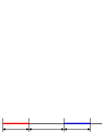
Figure 1: Schematic illustration of two time intervals and their time separation.

To calculate the time correlation function of the particle dynamics, we performed MD simulations in three dimensions on binary mixtures of two different atomic species, 1 and 2, with $N_{1}=N_{2}=5,000$ particles and a cube of constant volume $V$ as the basic cell, surrounded by periodic boundary image cells. The particles interact via the soft-sphere potentials $v_{ab}(r)=\epsilon(\sigma_{ab}/r)^{12}$, where r is the distance between two particles, $\sigma_{ab}=(\sigma_{a}+\sigma_{b})/2$, and $a,b\in 1,2$. The interaction was truncated at $r=3\sigma_{ab}$. In the present letter, the following dimensionless units were used: length, $\sigma_{1}$; temperature, $\epsilon/k_{B}$; and time, $\tau_{0}=(m_{1}\sigma_{1}^{2}/\epsilon)$. The mass ratio was $m_{2}/m_{1}=2$, and the diameter ratio was $\sigma_{2}/\sigma_{1}=1.2$. This diameter ratio avoided system crystallization and ensured that an amorphous supercooled state formed at low temperatures miyagawa_1991 . The particle density was fixed at the high value of $\rho=(N_{1}+N_{2})\sigma_{1}^{3}/V=0.8$. The system length was $L=V^{1/3}=23.2\sigma_{1}$. Simulations were carried out at $T=0.772,\ 0.473,\ 0.352,\ 0.306,\ 0.289,\ 0.267$, and $0.253$. Note that the freezing point of the corresponding one-component model is around $T=0.772\ (\Gamma_{\text{eff}}=1.15)$ miyagawa_1991 . Here, $\Gamma_{\text{eff}}$ is the effective density, a single parameter characterizing this model. At $T=0.253\ (\Gamma_{\text{eff}}=1.52)$, the system is in a highly supercooled state. We used the leapfrog algorithm with time steps of $0.005\tau$ when integrating the Newtonian equation of motion. Very long annealing times ($3\times 10^{6}$ for $T=0.253$) were chosen. No appreciable aging effect was detected in various quantities, including the pressure or the density correlation function.

Figure 2: $\tau_{\alpha}$, $\tau_{\text{ngp}}$ versus inverse temperature $1/T$. We use these two time intervals to define the local dynamics.

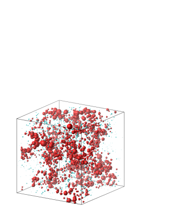
(a)

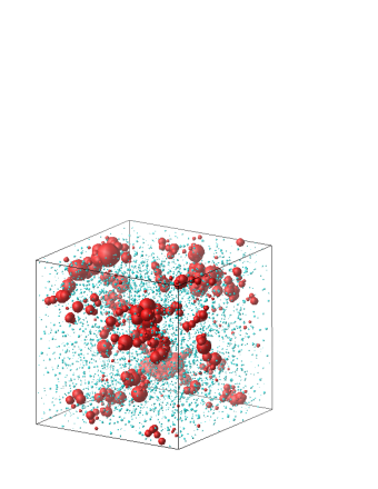
(b)

Figure 3: Visualization of the heterogeneous dynamics of particle species 1. The temperature is $0.253$. The time interval is $[t_{0},t_{0}+\tau_{\alpha}]$ in (a), $[t_{0},t_{0}+\tau_{\text{ngp}}]$ in (b). The radii of the spheres are $\left|\Delta\mbox{\boldmath$r$}_{j}(t_{0},t)\right|^{2}/{\langle[\Delta\mbox{\boldmath$r$}_{j}(t_{0},t)]^{2}\rangle}$, and the centers are at $\frac{1}{2}[\mbox{\boldmath$r$}_{j}(t_{0})+\mbox{\boldmath$r$}_{j}(t_{0}+t)]$. The red spheres and blue spheres represent $\left|\Delta\mbox{\boldmath$r$}_{j}(t_{0},t)\right|^{2}/{\langle[\Delta\mbox{\boldmath$r$}_{j}(t_{0},t)]^{2}\rangle}\geq 1$ and $\left|\Delta\mbox{\boldmath$r$}_{j}(t_{0},t)\right|^{2}/{\langle[\Delta\mbox{\boldmath$r$}_{j}(t_{0},t)]^{2}\rangle}<1$, respectively.

To define the local dynamics, we consider the two time intervals, $\tau_{\alpha}$ and $\tau_{\text{ngp}}$. $\tau_{\alpha}$ is the $\alpha$ relaxation time defined by $F_{s}(k_{m},\tau_{\alpha})=e^{-1}$, where $F_{s}(k,t)$ is the self-part of the density time correlation function for particle species 1, and $k_{m}=2\pi$ is the first peak wavenumber of the static structure factor. $\tau_{\text{ngp}}$ is the time at which the non-Gaussian parameter rahman_1964 of the van Hove self-correlation function is maximized. In Fig.2, we show $\tau_{\alpha}$ and $\tau_{\text{ngp}}$ as function of the inverse temperature $1/T$. $\tau_{\alpha}\simeq\tau_{\text{ngp}}$ at $T=0.306$, and $\tau_{\alpha}$ grows exponentially larger than $\tau_{\text{ngp}}$ with decreasing temperature at $T<0.306$. This trend agrees with other simulation results of Lennard-Jones (LJ) systems kob_1995_1 kob_1995_2 . Next, we visualize the heterogeneous dynamics of $\tau_{\alpha}$ and $\tau_{\text{ngp}}$ in the same manner presented in Ref.yamamoto_1998 . We calculate the displacement of each particle of species 1 in the time interval $[t_{0},t_{0}+t]$, $\Delta\mbox{\boldmath$r$}_{j}(t_{0},t)=\mbox{\boldmath$r$}_{j}(t_{0}+t)-\mbox{\boldmath$r$}_{j}(t_{0})\ (j=1,2,...,N_{1})$. In Fig.3, particles are drawn as spheres with radii

$$a_{j}^{2}(t_{0},t)=\frac{\left|\Delta\mbox{\boldmath$r$}_{j}(t_{0},t)\right|^{2}}{\langle[\Delta\mbox{\boldmath$r$}_{j}(t_{0},t)]^{2}\rangle}$$ (4)

located at $\mbox{\boldmath$R$}_{j}(t_{0},t)=\frac{1}{2}[\mbox{\boldmath$r$}_{j}(t_{0})+\mbox{\boldmath$r$}_{j}(t_{0}+t)]$ in both time intervals: $[t_{0},t_{0}+\tau_{\alpha}]$ ($t=\tau_{\alpha}$) in 3(a), $[t_{0},t_{0}+\tau_{\text{ngp}}]$ ($t=\tau_{\text{ngp}}$) in 3(b). The temperature is $0.253$. $a_{j}^{2}(t_{0},t)\geq 1$ ($a_{j}^{2}(t_{0},t)<1$) means that the particle $j$ moves more (less) than the mean value of the single-particle displacement. In Fig.3, the red (blue) spheres represent $a_{j}^{2}(t_{0},t)\geq 1$ ($a_{j}^{2}(t_{0},t)<1$). We can see the large-scale heterogeneities in both $\tau_{\alpha}$ and $\tau_{\text{ngp}}$.

Figure 4: The time decay of $S_{\mathcal{D}}(q,t_{s},t)$ at $t=\tau_{\alpha}$, $q=0.38$ for $T=0.772$ - $0.253$. $q=0.38$ is the smallest wavenumber in our simulation. Temperature decreases going right.

Figure 5: The wavenumber dependence of $\tau_{h}(q,t)$ at $t=\tau_{\alpha}$ for $T=0.772-0.253$. Temperature decreases going up. The dotted line is $\tau_{h}(q,\tau_{\alpha})\sim q^{-2}$

We can quantify the lifetimes of the heterogeneous dynamics in both time intervals. We consider the local fluctuations in the particle dynamics defined by

$$\delta\mathcal{D}(\mbox{\boldmath$q$},t_{0},t)=\sum_{j=1}^{N_{1}}(a_{j}^{2}(t_{0},t)-1)\exp[-i\mbox{\boldmath$q$}\cdot\mbox{\boldmath$R$}_{j}(t_{0},t)],$$ (5)

which is equal to the fluctuations in the diffusivity density defined in ref yamamoto_1998 and represents the local fluctuations in the particle dynamics in the time interval $[t_{0},t_{0}+t]$. We use $\delta\mathcal{D}(\mbox{\boldmath$q$},t_{0},t)$ as $\delta Q_{{k}}(\mbox{\boldmath$q$},t_{0},t)$ in Eq.(2), and the time correlation function defined by

$$S_{\mathcal{D}}(q,t_{s},t)=\langle\delta\mathcal{D}(\mbox{\boldmath$q$},t_{s}+t,t)\delta\mathcal{D}(-\mbox{\boldmath$q$},0,t)\rangle,$$ (6)

corresponds to $F_{4,{k}}({q},t_{s},t)$. $S_{\mathcal{D}}(q,t_{s},t)$ represents the correlation of the particle dynamics between two time intervals $[0,t]$ and $[t_{s}+t,t_{s}+2t]$ (see Fig.1). Thus, we can estimate the lifetime of the heterogeneous dynamics by examining the time decay of $S_{\mathcal{D}}(q,t_{s},t)$. As the time separation $t_{s}$ increases, $S_{\mathcal{D}}(q,t_{s},t)$ with fixed $t$ decays in the stretched exponential form,

$$\frac{S_{\mathcal{D}}(q,t_{s},t)}{S_{\mathcal{D}}(q,0,t)}\sim\exp\left(-\left(\frac{t_{s}}{\tau_{h}(q,t)}\right)^{c}\right),$$ (7)

where $\tau_{h}(q,t)$ is the wavenumber-dependent heterogeneous dynamics lifetime, which corresponds to $\tau_{4,{k}}({q},t)$ in Eq.(3). Figure 4 shows the time decay of $S_{\mathcal{D}}(q,t_{s},t)$ at $t=\tau_{\alpha}$, $q=0.38$ for various temperatures. $q=0.38$ is the smallest wavenumber in our simulation. In Fig.5, we show the wavenumber dependence of $\tau_{h}(q,t)$ at $t=\tau_{\alpha}$. $\tau_{h}(q,\tau_{\alpha})$ depends on $q$ more weakly than the $q$-dependent relaxation time of the two-point density correlation functions and dramatically increases with decreasing temperature in a wide region of $q$ ($q=0.38-19$). Furthermore, we can see that $\tau_{h}(q,\tau_{\alpha})$ approaches $\tau_{h}(q,\tau_{\alpha})\sim q^{-2}$ at small wavenumbers. This suggests that the heterogeneous dynamics migrate in space with a diffusion-like mechanism. These results of $\tau_{h}(q,\tau_{\alpha})$ are qualitatively the same as those of $\tau_{h}(q,\tau_{\text{ngp}})$.

We determined the lifetime of the heterogeneous dynamics $\tau_{\text{hetero}}(t)$ as $\tau_{h}(q,t)$ at $q=0.38$, which is the time separation $t_{s}$ at which $S_{\mathcal{D}}(q,t_{s},t)/S_{\mathcal{D}}(q,0,t)$ at $q=0.38$ equals $e^{-1}$ in Fig.4. $\tau_{\text{hetero}}(t)$ increases dramatically with decreasing temperature. We plot $\tau_{\text{hetero}}(t)$ versus $\tau_{\alpha}$ in Fig.6, which shows that $\tau_{\text{hetero}}(\tau_{\alpha})\sim\tau_{\alpha}^{1.08}$ and $\tau_{\text{hetero}}(\tau_{\text{ngp}})\sim\tau_{\alpha}^{0.91}$. The difference between $\tau_{\text{hetero}}(\tau_{\alpha})$ and $\tau_{\text{hetero}}(\tau_{\text{ngp}})$ increases with decreasing temperature. At $T=0.253$, $\tau_{\text{hetero}}(\tau_{\alpha})\simeq 7.8\tau_{\alpha}$, and $\tau_{\text{hetero}}(\tau_{\text{ngp}})\simeq 1.4\tau_{\alpha}$. Therefore, $\tau_{\text{hetero}}(\tau_{\alpha})$ is considerably larger than $\tau_{\alpha}$, while $\tau_{\text{hetero}}(\tau_{\text{ngp}})$ is comparable to $\tau_{\alpha}$. The existence of a slower timescale in the heterogeneous dynamics is consistent with Ref.kim_2009 .

Figure 6: The lifetime $\tau_{\text{hetero}}(t)$ for $t=\tau_{\alpha}$, $\tau_{\text{ngp}}$ versus $\tau_{\alpha}$. The line $\tau_{\text{hetero}}=2.65\tau_{\alpha}^{1.08}$ is fitted for $t=\tau_{\alpha}$, while the line $\tau_{\text{hetero}}=3.75\tau_{\alpha}^{0.91}$ is fitted for $t=\tau_{\text{ngp}}$.

Finally, we examine the finite-size effect. To this end, we performed MD simulations using a larger system with $N_{1}=N_{2}=50,000$ and $L=50\sigma_{1}$, and compared our results with those of a larger system. No finite-size effect was detected in quantities such as $\tau_{\alpha},\ \tau_{\text{ngp}}$, or $\tau_{\text{hetero}}$.

In summary, we have investigated the heterogeneous dynamics in two different time intervals, $\tau_{\alpha}$ and $\tau_{\text{ngp}}$. We quantified the lifetimes of the heterogeneous dynamics in these two intervals, $\tau_{\text{hetero}}(\tau_{\alpha})$ and $\tau_{\text{hetero}}(\tau_{\text{ngp}})$, by calculating the time correlation function of the particle dynamics. We found that the difference between $\tau_{\text{hetero}}(\tau_{\alpha})$ and $\tau_{\text{hetero}}(\tau_{\text{ngp}})$ increases with decreasing temperature. At low temperatures, $\tau_{\text{hetero}}(\tau_{\alpha})$ is considerably larger than $\tau_{\alpha}$, while $\tau_{\text{hetero}}(\tau_{\text{ngp}})$ remains comparable to $\tau_{\alpha}$. Thus, we can conclude that the lifetime of the heterogeneous dynamics depends strongly on the time interval. We also have examined the finite-size effect. No finite-size effect was detected in our study.

References

(1)M. D. Ediger, C. A. Angell, and S. R. Nagel, J. Phys. Chem. 100, 13200 (1996)
(2)P. G. Debenedetti and F. H. Stillinger, Nature 410, 259 (2001)
(3)T. Muranaka and Y. Hiwatari, Phys. Rev. E 51, R2735 (1995)
(4)M. M. Hurley and P. Harrowell, Phys. Rev. E 52, 1694 (1995)
(5)R. Yamamoto and A. Onuki, Phys. Rev. E 58, 3515 (1998)
(6)R. Yamamoto and A. Onuki, Phys. Rev. Lett. 81, 4915 (1998)
(7)D. N. Perera and P. Harrowell, J. Chem. Phys. 111, 5441 (1999)
(8)A. W. Cooper, P. Harrowell, and H. Fynewever, Phys. Rev. Lett. 93, 135701–1 (2004)
(9)B. Doliwa and A. Heuer, J. Non-Cryst. Solids 307-310, 32 (2002)
(10)C. Donati, J. F. Douglas, W. Kob, S. J. Plimpton, P. H. Poole, and S. C. Glotzer, Phys. Rev. Lett. 80, 2338 (1998)
(11)W. K. Kegel and A. van Blaaderen, Science 287, 290 (2000)
(12)E. R. Weeks, J. C. Crocker, A. C. Levitt, A. Schofield, and D. A. Weitz, Science 287, 627 (2000)
(13)N. Laevi,
F. W. Starr, T. B. Schrøder, and S. C. Glotzer, J. Chem. Phys. 119, 7372 (2003)
(14)C. Toninelli, M. Wyart, L. Berthier, G. Biroli, and J. P. Bouchaud, Phys. Rev. E 71, 041505 (2005)
(15)R. S. L. Stein and H. C. Andersen, Phys. Rev. Lett. 101, 267802 (2008)
(16)M. D. Ediger, Annu. Rev. Phys. Chem. 51, 99 (2000)
(17)L. Berthier, G. Biroli, J. P. Bouchaud, L. Cipelletti, D. El Masri, D. L’Hote, F. Ladieu, and M. Pierno, Science 310, 1797 (2005)
(18)G. Biroli, J. P. Bouchaud, K. Miyazaki, and D. R. Reichman, Phys. Rev. Lett. 97, 195701 (2006)
(19)E. Flenner and G. Szamel, Phys. Rev. E 70, 052501 (2004)
(20)K. Kim and S. Saito, Phys. Rev. E 79, 060501(R) (2009)
(21)C. Y. Wang and M. D. Ediger, J. Phys. Chem. B 103, 4177 (1999)
(22)C. Y. Wang and M. D. Ediger, J. Chem. Phys. 112, 6933 (2000)
(23)H. Miyagawa and Y. Hiwatari, Phys. Rev. A 44, 8278 (1991)
(24)A. Rahman, Phys. Rev. 136, A405 (1964)
(25)W. Kob and H. C. Andersen, Phys. Rev. E 51, 4626 (1995)
(26)W. Kob and H. C. Andersen, Phys. Rev. E 52, 4134 (1995)