Two - dimensional solitons in media with the stripe - shaped nonlinearity modulation

Abstract

We introduce a model of media with the cubic attractive nonlinearity concentrated along a single or double stripe in the two-dimensional (2D) plane. The model can be realized in terms of nonlinear optics (in the spatial and temporal domains alike) and BEC. In recent works, it was concluded that search for stable 2D solitons in models with a spatially localized self-attractive nonlinearity is a challenging problem. We make use of the variational approximation (VA) and numerical methods to investigate conditions for the existence and stability of solitons in the present setting. The result crucially depends on the transverse shape of the stripe: while the rectangular profile supports stable 2D solitons, its smooth Gaussian-shaped counterpart makes all the solitons unstable. The double stripe with the rectangular profile admit stable solitons of three distinct types: symmetric and asymmetric ones with a single peak, and double-peak symmetric solitons. The shape and stability of single-peak solitons of either type are accurately predicted by the VA. Collisions between stable solitons are briefly considered too, by means of direct simulations. Depending on the relative velocity we observe excitation, decay or catastrophic self focusing.

I Introduction and model

The propensity of localized patterns (solitons) to the catastrophic self focusing in two-dimensional (2D) media with the self-attractive nonlinearity of the most fundamental cubic (Kerr) type is a well-known property which impedes the creation of 2D solitons in optics and/or Bose-Einstein condensates (BECs) 1 . It was theoretically predicted for Kerr media 5-8 and demonstrated experimentally in photorefractive crystals, whose nonlinearity is saturable 2-4 , that the stabilization of 2D solitons may be provided by periodic potentials, which can be created as optical lattices.

A different stabilization mechanism for 2D solitons was theoretically elaborated in the form of nonlinear lattices Sivan ; HS ; Barcelona , i.e., a spatially periodic or localized modulation of the nonlinearity. In BEC this setting may be induced by dint of the Feshbach resonances controlled through nonuniform magnetic fields SU . In optics, similar media may be structured as liquid-crystal-filled liquid-crystal or all-solid all-solid microstructured fibers, using combinations of materials matched in their refractive index but featuring different Kerr coefficients. Actually, even in theoretical studies the stabilization of 2D solitons by the spatial modulation of the cubic nonlinearity is a difficult problem. In particular, it was not possible to find stable 2D solitons supported by spatially periodic nonlinear lattices similar to their linear counterpart which readily stabilize the solitons. Quasi-1D nonlinear lattices, i.e., nonlinearity-modulation profiles which periodic functions of a single coordinate, give rise to a tiny stability area for 2D solitons, suggesting a conclusion that this mechanism is irrelevant to physical applications Sivan (while quasi-1D linear lattices easily create stable solitons in a sizeable parameter region Q1D ). In fact, the only nonlinear 2D structures that have thus far produced positive results as concerns the soliton stability are represented by a circle filled with the nonlinear material, which is embedded into a linear or defocusing nonlinear medium HS , and a lattice of such circles Barcelona . In particular, it was concluded that the nonlinearity-modulation profile with sharp edges (such as those of the circles) provide for an essentially better stabilization of 2D solitons than smooth profiles.

The objective of the present work is to investigate possibilities to create stable 2D solitons by the nonlinearity concentrated along a single or double quasi-1D stripe, rather than patterned as a periodic lattice. It will be demonstrated that these settings give rise to a finite stability areas for several types of 2D solitons, on the contrary to the negligible stabilization region supported by the quasi-1D periodic lattice Sivan . The results will be obtained in a semi-analytical form using an appropriate variational approximation (VA), and, in parallel, by means of numerical methods.

Following Refs. HS -Barcelona , the general scaled form of the 2D equation with the stripe-shaped modulated nonlinearity can be written as

$$i\psi_{t}=-\left(1/2\right)\left(\psi_{xx}+\psi_{yy}\right)+g(x)\left|\psi\right|^{2}\psi.$$ (1)

In this work, we consider three forms of the quasi-1D modulation of coefficient $g(x)\leq 0$ accounting for the self-attractive nonlinearity: the Gaussian,

$$g(x)=-\exp\left(-x^{2}\right),$$ (2)

a single rectangular box,

$$g(x)=\left\{\begin{array}[]{ll}-1&\mbox{at }~{}~{}|x|\leq 2,\\ 0&\mbox{at }~{}~{}|x|>2,\end{array}\right.$$ (3)

and two symmetrically set boxes:

$$g(x)=\left\{\begin{array}[]{ll}-1&\mbox{ at }~{}~{}d-1\leq|x|\leq d+1,\\ 0&\mbox{ at }~{}~{}|x|>d+1,~{}|x|<d-1.\end{array}\right.$$ (4)

In all these cases, the coefficients may be fixed to their values adopted in Eqs. (1)-(4) by means of rescalings, i.e., the modulation profiles (2) and (3) have no free parameters, while their double-box counterpart (4) depends on a single parameter, $d>1$, which measures half of the distance between centers of the boxes, whose width is fixed to be $2$. Notice, that if $d<1$ we are dealing effectively with a single box.

In the application to BEC, Eq. (1) is the scaled Gross-Pitaevskii equation for the mean-field wave function, $\psi\left(x,y,t\right)$ HS -Barcelona . In optics, the same model admits two different realizations. With $t$ replaced by the propagation distance, $z$, Eq. (1) may be considered as the nonlinear Schrödinger (NLS) equation to govern the transmission of light beams in the bulk linear ambient medium, with the transverse structure induced by an embedded nonlinear slab [Eqs. (2) or (3)], or two parallel slabs, in the case of Eq. (4). On the other hand, the same equation (1), with $t$ replaced by $z$ and $y$ replaced by the temporal variable, $\tau\equiv t-z/c$, where $c$ is the group velocity of the carrier wave, describes the transmission of spatiotemporal optical signals (alias 2D light bullets 1 ) in a planar linear waveguide, with an embedded nonlinear single or double stripe. Accordingly, stable 2D solitons reported in this paper are interpreted as solitary pulses of matter waves in the BEC, or spatial solitons in the bulk optical medium, or, finally, as the light bullets guided in the planar medium. Stationary soliton solutions are sought for as $\psi(x,y,t)=e^{-i\mu t}\phi(x,y)$, where $\mu$ is the chemical potential (in terms of BEC), and function $\phi(x,y)$ satisfies equation

$$\mu\phi+\left(1/2\right)\left(\phi_{xx}+\phi_{yy}\right)-g(x)|\phi|^{2}\phi=0.$$ (5)

Equation (1) conserves the norm, $N=\int\int|\psi(x,y)|^{2}dxdy,$ which will play the role of an intrinsic parameter of soliton-solution families. In BEC, $N$ is proportional to the total number of atoms, while in the bulk and planar optical waveguides it measures, respectively, the total power or energy. Equation (1) also conserves the Hamiltonian and $y$-component of the momentum,

$$H=\frac{1}{2}\int\int\left[\left(\left|\psi_{x}\right|^{2}+\left|\psi_{y}\right|^{2}\right)+g(x)|\psi|^{4}\right]dxdy,$$ (6)

$$P=i\int\int\left(\psi_{x}^{\ast}\psi-\psi_{x}\psi^{\ast}\right)dxdy.$$ (7)

For the application of the VA, it is relevant to mention that Eq. (5) may be derived from the Lagrangian,

$$L=\int\int\left[\mu|\phi|^{2}-\frac{1}{2}\left(|\phi_{x}|^{2}+|\phi_{y}|^{2}\right)-\frac{1}{2}g(x)|\phi|^{4}\right]dxdy.$$ (8)

The rest of the paper is organized as follows. The solitons supported by the Gaussian profile (2) are considered in Section II, where it is demonstrated that they all are unstable. Stable solitons are found in Sections III and IV, in the models based on the single- and double-box modulation profiles (3) and (4), respectively. In these sections, the VA and numerical methods are used in parallel. In particular, three types of solitons are found in the setting based on the double stripe: symmetric and asymmetric ones with a single peak, and double-peak symmetric solitons. All the soliton species have their stability regions (for the double-peak soliton, it is very narrow). In Section V, collisions between solitons are studied by means of direct simulations. The paper is concluded by Section VI.

II The stripe with the Gaussian profile

We start the analysis by considering 2D solitons supported by the modulation profile (2). First, we apply the VA based on the natural ansatz of the Gaussian type too, with widths $a$ and $b$:

$$\phi(x,y)=A\exp\left[-\left(1/2\right)\left(a^{2}x^{2}+b^{2}y^{2}\right)\right],$$ (9)

whose norm is $N=\int\int\phi^{2}(x,y)dxdy=\pi A^{2}/\left(ab\right).$The substitution of the ansatz into Hamiltonian (6) yields the following expression, where the squared amplitude, $A^{2}$, is eliminated in favor of $N$:

$$H=\frac{N}{4}\left(a^{2}+b^{2}-\frac{\sqrt{2}Na^{2}b}{\pi\sqrt{1+2a^{2}}}\right).$$ (10)

The variational equations for parameters $a$ and $b$, $\partial H/\partial a=\partial H/\partial b=0$ yield a system of algebraic equations for $a$ and $b$:

$$\pi(1+2a^{2})^{3/2}-\sqrt{2}Nb(1+a^{2}) = 0,$$ (11)

$$\pi b\sqrt{2\left(1+2a^{2}\right)}-a^{2}N = 0.$$ (12)

Equation (12) can be used to eliminate parameter $b$:

$$b=a^{2}N/\left[\pi\sqrt{2(1+2a^{2})}\right].$$ (13)

Substituting this into Eq. (11), we derive a quadratic equation for $a^{2}$:

$$a^{2}(1+a^{2})=\left(\pi/N\right)^{2}(1+2a^{2})^{2}.$$ (14)

A physical (positive) root of Eq. (14) is

$$a^{2}=\frac{N}{2\sqrt{N^{2}-4\pi^{2}}}-\frac{1}{2},$$ (15)

which predicts that the 2D solitons exist provided that the norm exceeds a threshold value, $N_{\mathrm{thr}}=2\pi$. In fact, the same generic feature of solitons was found in other models based on the spatial modulation of the nonlinearity, both two- HS ; Sivan ; Barcelona and one-dimensional 1D .

Further, we insert $b$ and $a$ from Eqs. (13) and (15) into Eq. (10) to obtain the expression for the Hamiltonian predicted by the VA:

$$H=\frac{N}{16\pi^{2}}\left[N\left(N-\sqrt{N^{2}-4\pi^{2}}\right)-2\pi^{2}\right].$$ (16)

Using the definition of the chemical potential, $\mu=dH/dN$, the Vakhitov-Kolokolov (VK) criterion VK , $d\mu/dN<0$, which is assumed to be a necessary condition for the stability of the solitons, is then cast in the form of

$$d^{2}H/dN^{2}<0.$$ (17)

From (16) we obtain

$$\frac{d^{2}H}{dN^{2}}=\frac{1}{8\pi^{2}}\left[3N+\frac{16\pi^{2}N^{2}-3N^{4}-16\pi^{4}}{(N^{2}-4\pi^{2})^{3/2}}\right].$$ (18)

It is easy to check that this expression is always positive, hence the VA predicts that the 2D solitons supported by the stripe-shaped modulation of the attractive nonlinearity with the Gaussian profile cannot be stable. We also calculated the matrix of second order derivatives of the Hamiltonian with respect to $a$ and $b$ and check that the stationary point (solution of Eqs. (11) and (12)) is not a minimum. Direct simulations (not shown here) corroborate this prediction: no stable 2D solitons can be found in the model based on Eqs. (1) and (2).

III The modulation stripe with the box-shaped profile

III.1 The variational approximation

Proceeding to the model with the rectangular modulation profile (3), we again start with the VA, using two different ansätze, namely, the same Gaussian-shaped one as in Eq. (9), and also the product of hyperbolic secants:

$$\phi(x,y)=A~{}\mathrm{sech}(x/a)\mathrm{sech}(y/b),$$ (19)

whose norm is $N=4A^{2}ab$. An ansatz of the latter type was originally used for modeling multidimensional solitons in Ref. Japan .

The substitution of ansatz (19) into Lagrangian (8) yields

$$L = 4A^{2}ab\mu-\frac{2A^{2}(a^{2}+b^{2})}{3ab}$$

$$+ \frac{2}{9}abA^{4}\mathrm{sech}^{3}\left(\frac{2}{a}\right)\left[3{\sinh}\left(\frac{2}{a}\right)+{\sinh}\left(\frac{6}{a}\right)\right].$$

Deriving the Euler-Lagrange equations from this expression, it is possible to eliminate $A$ and $b$, ending up with equations

$$\mu=\frac{1}{3a^{2}}\left[\frac{36}{24+4a~{}{\sinh}(\frac{4}{a})+a~{}{\sinh}(\frac{8}{a})}-1\right],$$ (21)

$$N=\frac{12a~{}{\cosh}^{2}(\frac{2}{a}){\coth}(\frac{2}{a})}{\left[2+{\cosh}(\frac{4}{a})\right]\sqrt{a\left\{a+24\left[4{\sinh}(\frac{4}{a})+{\sinh}(\frac{8}{a})\right]^{-1}\right\}}}.$$ (22)

The system of Eqs. (21) and (22) was solved numerically. Curves $N(\mu)$ for the soliton families, produced by the ansätze of both types, are shown in Fig. 1. According to the VK criterion, portions of the soliton families depicted by the solid curves may be stable.

The Hamiltonian corresponding to ansatz (19) is

$$H=\frac{N}{6}\left(\frac{1}{a^{2}}+\frac{1}{b^{2}}\right)-\frac{N^{2}}{36ab}\left[2+\mathrm{sech}^{2}\left(\frac{2}{a}\right)\right]{\tanh}\left(\frac{2}{a}\right),$$ (23)

cf. Eq. (16). Again the stability condition obtained from Fig. 1 using VK criterion coincide with the fact that the Hamiltonian (23) has a local minimum.

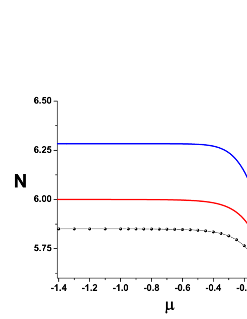
Figure 1: (Color online) Curves $\mu(N)$ for the soliton family, as predicted by the variational approximations based on the sech-sech ansatz (19) (red) and Gaussian (9) (bue), in the  model with the single-box modulation profile (3). The VK-stable portions of the family are shown by solid curves. Numerically found stable solitons are shown by the chain of circles.

III.2 Numerical results

We have performed systematic numerical simulations of Eqs. (1), (3), with the aim to verify the predictions of the VA for this model. First, stationary shapes of 2D solitons were generated by means of imaginary-time simulations. Then, their stability was checked using the split-step Fourier-transform method for simulating the evolution of perturbed solitons, to which a small disturbance was added. The initial perturbation changed the total norm of the soliton by up to $0.1\%$ (adding perturbations at this level were sufficient to clearly distinguish between stable and unstable solitons).

The simulations produce stable 2D solitons in the interval of $5.645\leq N\leq 5.85$. The comparison of the numerical findings with the predictions of the VA is shown in the Figure 1.
The fact that the replacement of the smooth Gaussian modulation profile by the box-shaped one agrees with the above-mentioned general trend discovered in other models dealing with the spatially modulated nonlinearity, viz., that modulation profiles with sharp edges are more apt to generate stable 2D solitons than their smoothly shaped counterparts HS ; Barcelona .

IV The double-box modulation profile

IV.1 The variational approximation

To consider the model based on the dual-box modulation profile as given by Eq. (4), we have started with the VA based on the factorized-sech ansatz similar to that introduced above in the form of Eq. (19), but with an additional degree of freedom, $c$, which makes it possible to consider solitons configurations with a spontaneously broken symmetry:

$$\phi(x,y)=\frac{1}{2}\sqrt{\frac{N}{ab}}\mathrm{sech}\left(\frac{x-c}{a}\right)\mathrm{sech}\left(\frac{y}{b}\right).$$ (24)

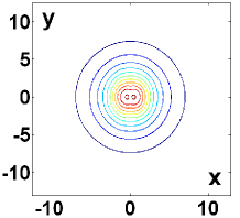
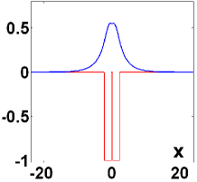
Figure 2: (Color online) An example of a stable double-peak symmetric soliton, with $N=6.82$, $\mu=-0.05$, and $d=1.2$. Left: A top view shown by means of contour plots; Right: the section drawn through $y=0$.

The respective expression for Hamiltonian (6) is:

$$H = \frac{N^{2}}{72ab}\left[\left(2+\mathrm{sech}^{2}\left(\frac{d+1-c}{a}\right)\right){\tanh}\left(\frac{c-1-d}{a}\right)-\left(2+\mathrm{sech}^{2}\left(\frac{c+1-d}{a}\right)\right){\tanh}\left(\frac{c+1-d}{a}\right)\right.$$

$$+ \left.\left(2+\mathrm{sech}^{2}\left(\frac{d+c-1}{a}\right)\right){\tanh}\left(\frac{c+d-1}{a}\right)-\left(2+\mathrm{sech}^{2}\left(\frac{c+1+d}{a}\right)\right){\tanh}\left(\frac{c+1+d}{a}\right)\right]+\frac{N}{6}\left(\frac{1}{a^{2}}+\frac{1}{b^{2}}\right).$$

In the model with the dual-trough linear potential, formally similar to its nonlinear counterpart (4), the spontaneous symmetry breaking of 2D solitons was studied in detail in Ref. we . In a 1D model with the nonlinearity modulation represented by two symmetric delta-functions, or by a superposition of two Gaussians, symmetry-breaking localized states were investigated in Ref. Dong .

The variational equations following from expression (LABEL:complex) are cumbersome, therefore they are not explicitly written here. These equations were solved numerically, for both symmetric ($c=0$) and asymmetric ($c\neq 0$) configurations. The stability condition following from the VA was implemented as a condition that the Hamiltonian must attain a local minimum at stationary points. The results are presented below, in comparison with respective numerical findings obtained from Eqs. (1) and (4).

IV.2 Basic types of two-dimensional solitons. Numerical results.

Numerical solutions for stationary 2D solitons were obtained by means of two numerical methods, namely, the imaginary-time integration (as above), and the spectral renormalization method MZ . In the former case, we fixed $N$ and aimed to find the corresponding value of $\mu$, while the latter algorithm was used to find $N$ corresponding to given chemical potential $\mu$.

Soliton solutions of three types have been found in this way: (i) symmetric modes with a single peak; (ii) asymmetric solutions with a single peak; and (iii) symmetric solitons with a double peak. Solutions with two asymmetric peaks have not been found. Obviously, modes of type (iii) cannot be predicted by the variational ansatz (24) (a modification of the ansatz that would incorporate double-peak patterns leads to an extremely messy algebra).

IV.2.1 Symmetric solitons with a single peak

In the case of $d\leq 1$, the two boxes in modulation profile (4) actually merge into one, bringing us back to profile (3) that was considered above. Accordingly, symmetric single-peak solitons are found in this case. At $d>1$, there is a small region where the VA predicts stable solutions. However, the full numerical solutions do not reveal any stationary modes of this type.

IV.2.2 Double-peak symmetric solitons

In the interval of $1<d\leq 1.2$, the spectral renormalization method MZ has produced stationary symmetric solutions with double peaks and a very shallow local minimum between them, see Fig. 2 (the imaginary-time method does not converge in this region). These solitary modes are stable only at very small values of $|\mu|$, when the solitons are very broad. For example, fixing $\mu=-0.05$, we have found that stable double-peak symmetric solutions exist in the interval of $1.1\leq d\leq 1.2$, where the dependence of $N$ on $\left(d-1\right)$ turns out to be linear, see Fig. 3. It may be relevant to note that, because the stability of the solitons was identified by means of direct simulations, it may happen that the stable solitons are, strictly speaking, subject to an extremely weak instability. Nevertheless, they are definitely stable modes in terms of physical applications.

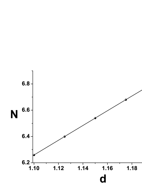
Figure 3: (Color online) The norm of the stable symmetric double-peak solitons versus the half-distance, $d$, between the two boxes in modulation profile (4), for a fixed chemical potential, $\mu=-0.05$.

IV.2.3 Asymmetric single-peak solutions

The system with the double-box modulation profile, given by Eq. (4) with $d>1$, can support asymmetric solutions with a single peak. Figures 4 and 5 display the form of stationary wave functions in two cases, with $d$ close to and far from $1$, respectively.

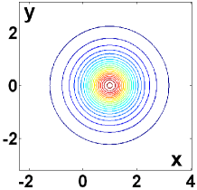
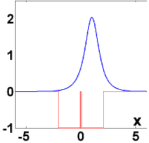
Figure 4: (Color online) The same as in Fig. 2, but for a stable asymmetric soliton with $N=5.8$, $\mu=-0.84$, and $d=1.05$. The substrate (red) line in the bottom panel represents the two-box profile (4).

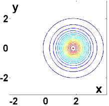
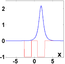
Figure 5: The same as in Fig. 4, but for a stable asymmetric soliton with $N=5.8$, $\mu=-0.962$, and $d=1.8$.

The asymmetry of solutions may be naturally characterized by parameter

$$\nu=\frac{\int_{-\infty}^{\infty}{d}y\int_{-\infty}^{0}{d}x|\phi(x,y)|^{2}-\int_{-\infty}^{\infty}{d}y\int_{0}^{\infty}{d}x|\phi(x,y)|^{2}}{N}.$$ (26)

In Fig. 6 we present curves $N(\mu)$ and $\nu(\mu)$ for the asymmetric solitons in the case of $d=1.2$. From these plots, and similar ones obtained at other values of $d$, it is concluded that the VA based on ansatz (24) provides for a good accuracy, in the comparison with numerical results.

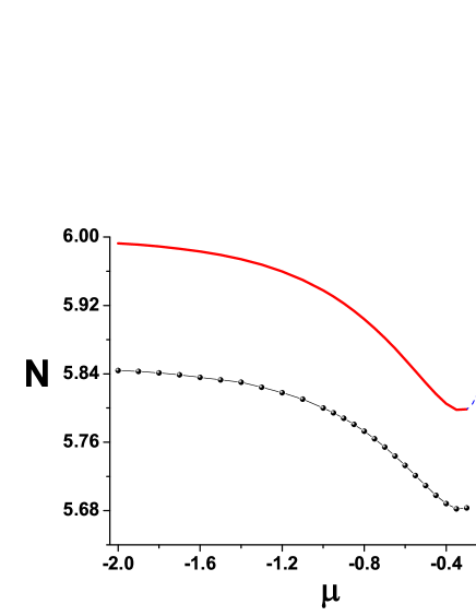
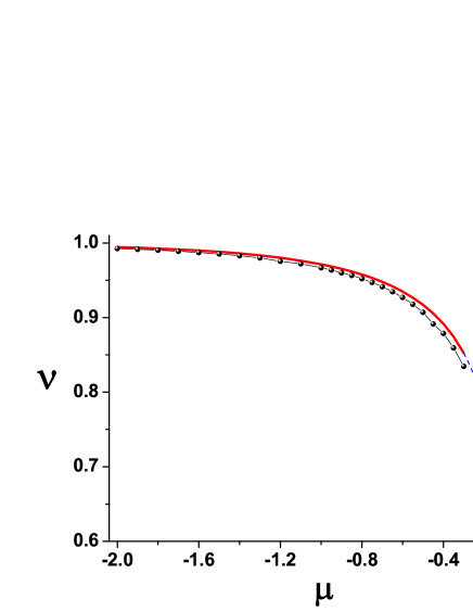
Figure 6: (Color online) Curves showing the norm and asymmetry parameter, $N(\mu)$ and $\nu(\mu)$, for asymmetric single-peak 2D solitons in the case of $d=1.2$. We display the comparison between the results predicted by the variational approximation (continuous/dashed curves, which depict stable/unstable portions of the soliton family), and their numerical counterparts (chains of circles).

IV.3 Stability and symmetry-breaking diagrams

The results produced by the VA and gleaned from full numerical solutions are collected in the form of stability diagrams displayed in Figs. 7 and 8. It is concluded that the numerically found stability areas (covered by black oblique lines in the figures) are shifted somewhat downward, against the variational predictions (covered by red oblique lines). Around $d=1$, there is a gap in the numerically found stability areas for the symmetric and asymmetric single-peak solitons. It is extremely difficult to fill this gap using direct numerical solutions, as the simulations necessary to check both the existence and stability of the solutions turn out to be very long in this case.

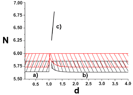
Figure 7: (Color online) The full stability diagrams for 2D solitons in the plane of $(d,N)$. In areas a) and b), stable solutions are, respectively, symmetric and asymmetric single-peak solitons (black and red areas depict the stability areas as produced, severally, by the numerical and variational methods). In a very thin area c), stable symmetric double-peak solutions have been found, in the numerical form.

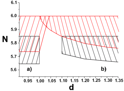
Figure 8: (Color online) A zoom of the stability diagram from Fig. 7 close to $d=1$, where the single-box modulation profile (3) goes over into the double-box shape (4).

Further, a symmetry-breaking diagram is displayed in Figs. 9 and 10. To produce this plot, we fixed the norm of the solitons and varied the half-distance, $d$, between the two wells. This implies that we keep a constant strength of the nonlinearity, while making the coupling between the two box-shaped stripes weaker. The norm of the solutions corresponding to the chain of circles in Figs. 9 and 10, which were found as numerical solutions to Eqs. (1), (4), was set as $N_{\mathrm{num}}=5.8$. The constant norm of the variational solutions presented in the same figures was fixed to be slightly different, $N_{\mathrm{VA}}=5.95$, as Fig. 1 suggests a correction ratio, $6/5.85\approx 5.95/5.8$ between the VA-predicted solutions and their numerically found counterparts.

The detailed picture of the symmetry-breaking transition, displayed in Fig. 10 demonstrates that the VA predicts the transition of a slightly subcritical type, with a narrow bistability region (coexistence of stable symmetric and asymmetric states) observed at $1.015<d<1.034$ (cf. Ref. we , where the subcritical transition and bistability were demonstrated in the 2D model with the double-trough linear potential). However, after reaching the destabilization point at $d=1.034$, the line of the symmetric solitons does not continue to larger values of $d$, as one might “naively” expect. Instead, the destabilized branch of the symmetric solitons turns back, running parallel to the stable one. The latter feature corresponds to the existence of the pair of stable and unstable solution branches in the model with the single-box modulation profile, see Fig. 1. These features of the symmetry-breaking diagram somewhat resembles those reported in Ref. Zeev , which was dealing with a 2D model combining the double-trough linear potential and the cubic-quintic nonlinearity. As concerns the stable and unstable VA-predicted branches of the asymmetric solutions, it may be expected that they will meet in the limit of large $d$, as in that limit each of the two boxes becomes equivalent to the one in the model with the single-box modulation profile.

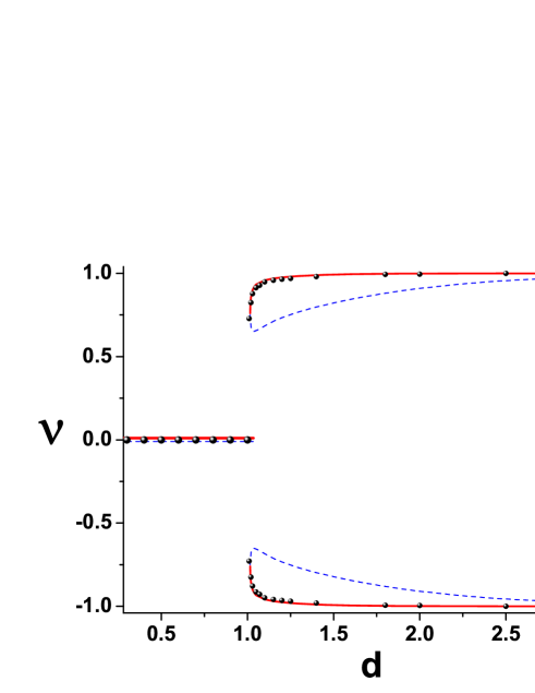
Figure 9: (Color online) The symmetry-breaking diagram, displayed as the $\nu(d)$ curve for a fixed norm of symmetric and asymmetric single-peak solitons, see the text. The red (continuous) and blue (dashed) curves depict, respectively, stable and unstable solutions predicted by the VA, while chains of circles represent numerically found stable solutions.

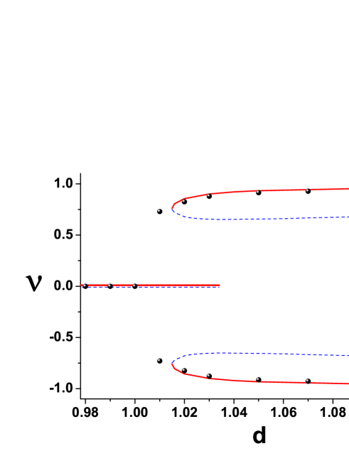
Figure 10: (Color online) A blow-up of the symmetry-breaking region from Fig. 9.

Numerical solutions for symmetric solitons have also been found at some values of $d>1$. However, the corresponding points are not shown in Fig. 10, as it was too difficult to resolve their stability.

Another representative stability and symmetry-breaking diagram can be constructed by varying the norm, $N$ (i.e., the nonlinearity strength, as a matter of fact) at a fixed value of the half-distance $d$ between the boxes. This diagram and a zoom of its most essential area are displayed in Figs. 11 and 12. The narrow interval of values of $N$ in which stable solitons, supported by the spatially modulated nonlinearity, may be found, is a generic feature of 2D models HS ; Sivan ; Barcelona . A noteworthy feature of this diagram is the absence of symmetric single-peak solutions (while their stable double-peak counterparts exist in a very narrow interval). The stable asymmetric solitons are obviously generated by saddle-node (subcritical) bifurcations. Unlike the 1D model with the double-stripe nonlinearity modulation Dong , here the existence regions for the stable solitons is bounded from above, in terms of $N$, by the catastrophic self focusing.

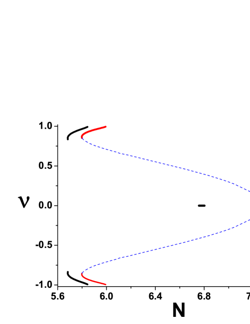
Figure 11: (Color online) The symmetry-breaking and stability diagram represented by the $\nu(N)$ curve for fixed $d=1.2$. The red (solid) and blue (dashed) curves depict, respectively, stable and unstable subfamilies of asymmetric single-peak solitons, as generated by the VA. The segments of black curves at the top and bottom represent stable solitons of the same type, obtained in the numerical form. The short black segment at the center depicts a family of stable symmetric double-peak solutions.

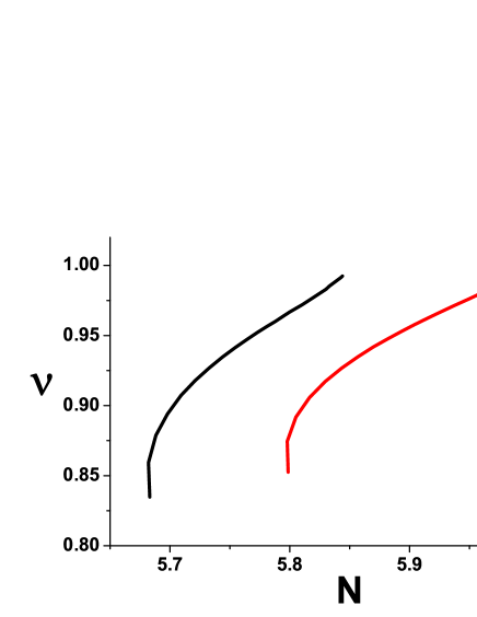
Figure 12: (Color online). A zoom of the part of Fig. 11 which shows in detail the variational (the red curve) and numerical (the black curve) families of stable asymmetric single-peak solitons.

V Collisions between moving solitons

In the last paragraph we report our studies on the soliton collisions. In this case soliton are moving along free direction, transverse to the nonlinearity modulation direction. We consider two collision scenarios. One occurs when colliding entities are moving in single rectangular box, and the other when they move along two different boxes in a double-box modulation profile. In both case we observe the same diagram of the collision results. For velocities above a critical value the solitons come out from the collision being excited - the collision is inelastic. The process of excitation is accompanied by some radiation. The amplitude of the excitation grows as we approach critical velocity. If we go below the critical velocity the solitons do survive the collision, but soon after they pass though each other, excitation turns into instability and the soliton gradually dissolve. If we decrease the velocity even further we eventually enter the region when the interaction time is long enough for the catastrophic self focusing to arise.

First we considered the case when nonlinearity modulation function is of the form of a single rectangular box (see Eq. (3)). Stable solitons in this case exist only for the value of the norm between $5.645$ and $5.85$ as we know from previous considerations (see Sec. III, Fig. 1). Three generic type of dynamics described above are shown in Fig. 13. The plot of critical velocity versus norm of each of the soliton is presented in Fig. 14. The nonmonotonic behavior can be understood as know that single soliton is least stable at the borders of its existence region. In the case of double-box modulation profile we in principle see the same kind of phenomena. We collide two asymmetric solitons which principal part is occupying different channels. The results are presented in Fig. 15.

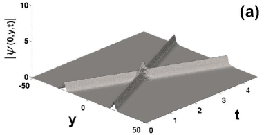
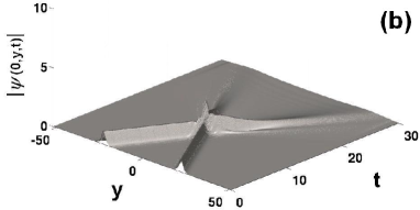
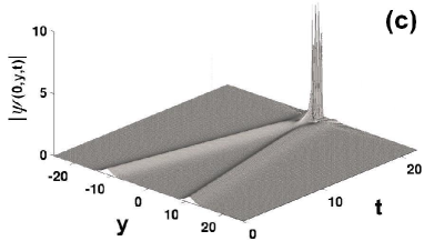
Figure 13: Collisions of solitons in a single box. Numerical data was obtained for $N=5.8$. Sections of the wavefunction along $y$ axis are shown for (a) $v=10$ (excitation), (b) $v=2$ (decay) and (c) $v=0.5$ (catastrophic self focusing) respectively.

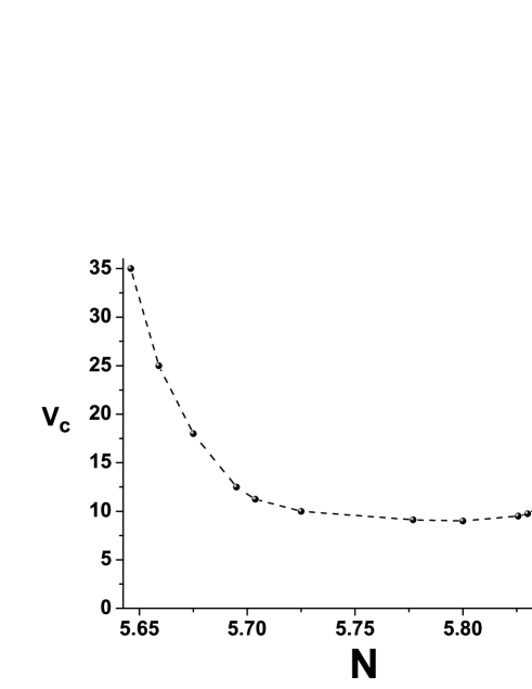
Figure 14: Critical velocity versus norm in the case of the single box collision.

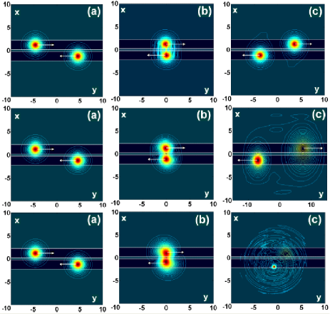
Figure 15: Contour plots illustrating soliton collisions in a double box. Numerical results were obtained for $N=5.8$ and $d=1.2$. Three figures in the each row show contours of the wavefunction (a) before, (b) during and (c) after the collision. The top row corresponds to $v=4$. The solitons get excited because of the collision. The middle row corresponds to $v=1$, where the solitons decay after the collision. Bottom row corresponds to $v=0.5$, where we observe catastrophic self focusing.

VI Conclusions

In this work, we have considered 2D solitons in the model of the medium with the self-attractive nonlinearity whose strength is subject to the spatial modulation in the form of a single or double stripe. The model may be implemented in BEC and nonlinear optics. It is known that the stabilization of 2D solitons by means of the spatial modulation of the self-attractive nonlinearity is a challenging problem. Using the combination of the variational approximation and direct simulations, we have found that the ability of the stripe-shaped modulation to stabilize the solitons crucially depends on its shape: while a smooth modulation profile in the form of a Gaussian does not support any stable 2D soliton, the rectangular (box-shaped) profile, as well as its double-box counterpart, give rise to stable solitons. In the case of the double stripe, three species of stable soliton solutions were found, viz., the single-peak symmetric and asymmetric solutions, and double-peak symmetric ones. Single-peak solitons of both symmetric and asymmetric types are accurately described by the VA, and their stability is adequately accounted for by the VK criterion. The symmetric double-peak solitons were found in a numerical form, turning out to be stable in a small region. Collisions between stable solitons were studied too, by means of direct simulations. We studied collisions in single and double rectangular boxes. Depending on the colliding partners velocity we observed three types of behavior: emerging solitons get some excitations for large velocity, for smaller velocity they decay (excitations were large enough to cause instability), and for even smaller velocity we enter the region where catastrophic self focusing occurs.

A challenging direction for the extension of the analysis reported in this work is to search for stable solitons supported by spatial modulations of the nonlinearity in the 3D space.

VII Acknowledgement

The authors acknowledge support of the Polish Government Research Grants for years 2007 2009 (N. V. H. and M.T.) and for years 2007 2010 (P.Z). The work of B. A. M. was supported, in a part, by the German - Israel Foundation through grant No. 149/2006.

References

- (1) B. A. Malomed, D. Mihalache, F. Wise, and L. Torner, J. Opt. B 7, R53 (2005).
- (2) B. B. Baizakov, B. A. Malomed, and M. Salerno, Europhys. Lett. 63, 642 (2003); J. Yang and Z. H. Musslimani, Opt. Lett. 28, 2094 (2003); H. Sakaguchi and B. A. Malomed, Europhys. Lett. 72, 698 (2005).
- (3) J. W. Fleischer, M. Segev, N. K. Efremidis, and D. N. Christodoulides, Nature 422, 148 (2003); H. Martin, E. D. Eugenieva, Z. Chen, and D. N. Christodoulides, Phys. Rev. Lett. 92, 123902 (2004); R. Fischer, D. Tröger, D. N. Neshev, A. A. Sukhorukov, W. Królikowski, C. Denz, and Y. S. Kivshar, Phys. Rev. Lett. 96, 023905 (2006).
- (4) G. Fibich, Y. Sivan, and M. I. Weinstein, Physica D 217, 31 (2006); Y. Sivan, G. Fibich, and M. I. Weinstein, Phys. Rev. Lett. 97, 193902 (2006).
- (5) H. Sakaguchi and B.A. Malomed, Phys. Rev. E 73, 026601 (2006).
- (6) Y. V. Kartashov, B. A. Malomed, V. A. Vysloukh, and L. Torner, Opt. Lett. 34, 770 (2009).
- (7) T. Mayteevarunyoo, B. A. Malomed, and G. Dong, Phys. Rev. A 78, 053601 (2008).
- (8) H. Saito and M. Ueda, Phys. Rev. A 65, 033624 (2002).
- (9) F. Du, Y. Q. Lu, and S. T. Wu, Appl. Phys. Lett. 85, 2181 (2004); Y. Y. Huang , Y. Xu, and A. Yariv, ibid. 85, 5182 (2004); L. Scolari, T. T. Alkeskjold, J. Riishede, and A. Bjarklev, Opt. Exp. 13, 7483 (2005).
- (10) F. Luan, A. K. George, T. D. Hedley, G. J. Pearce, D. M. Bird, J. C. Knight, and P. S. J. Russell, Opt. Lett. 29, 2369 (2004); G. Bouwmans, L. Bigot, Y. Quiquempois, F. Lopez, L. Provino, and M. Douay, Opt. Exp. 13, 8452 (2005); L. M. Tong, L. L. Hu, J. J. Zhang, J. R. Qiu, Q. Yang, J. Y. Lou, Y. H. Shen, J. L. He, and Z. Z. Ye, ibid. 14, 82 (2006).
- (11) B. B. Baizakov, B. A. Malomed and M. Salerno, Phys. Rev. A 70, 053613 (2004); T. Mayteevarunyoo, B. A. Malomed, B. B. Baizakov, and M. Salerno, Physica D 238, 1439 (2009).
- (12) H. Sakaguchi and B. A. Malomed, Phys. Rev. E 72, 046610 (2005); Phys. Rev. A 81, 013624 (2010).
- (13) N. G. Vakhitov and A. A. Kolokolov, , Radiophys. Quantum. Electron. 16, 783 (1973).
- (14) K. Hayata and M. Koshiba, Phys. Rev. Lett. 71, 3275 (1993).
- (15) M. Matuszewski, B. A. Malomed, and M. Trippenbach, Phys. Rev. A 75, 063621 (2007).
- (16) M. J. Ablowitz and Z. H. Musslimani, Opt. Lett 30, 2140 (2005).
- (17) Z. Birnbaum and B. A. Malomed, Physica D 237, 3252 (2008).