Continuous history variable for programmable quantum processors

Abstract

In this brief note is discussed application of continuous quantum history (“trash”) variable for simplification of scheme of programmable quantum processor. Similar scheme may be tested also in other models of the theory of quantum algorithms and complexity, because provides modification of a standard operation: quantum function evaluation.

1 Preliminaries

It was discussed in [1], that programmable quantum computer may be universal only in approximate sense. On the other hand, such computer may approximate any operation with arbitrary precision, if to repeat an elementary step sufficient number of times (“timing”) [2, 3, 4]. In fact, such kind of universality is rather standard since first papers about quantum computational networks [5]. Experimental realizations of programmable quantum computers also may use similar idea [6].

Really, programmable quantum processor sometimes could be compared with usual classical computer, controlling sequence of applications of quantum gates. There is well known formal method of revision of a scheme of a classical computation into a model, compatible with quantum laws. It is possible first to use some reversible design of Turing machine [7]. The quantum mechanical model of such device is quite straightforward [8].

In quantum circuit model similar approach sometimes is denoted as “quantum function evaluation” [9], but it is rather classical idea with using instead of irreversible function $f(x)$ the reversible one on the pair of arguments, like $\tilde{f}:(x,y)\mapsto(x,f(x)\circleddash y)$, where for different domains of $x$ operator $\circleddash$ may be subtraction (in modular or usual arithmetics) or bitwise exclusive or (for binary case). The $\tilde{f}$ is reversible ($\tilde{f}$ is involution, viz $\tilde{f}^{(-1)}=\tilde{f}$) and

$$\tilde{f}:(x,0)\mapsto(x,f(x))$$ (1)

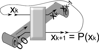
Figure 1: Scheme of tapes

But such a transition produces certain problem with “timing”. An initial irreversible computer might be considered as a sequence $M\to f(M)\to f(f(M))\cdots$, there $M$ is state of whole memory (containing both data and program) and $f$ is a fixed “function” corresponding to a circuits design.

For reversible function described above in Eq. (1) it is necessary on each step to provide new fresh input with zeros and to withdraw the redundant copy of $x$ from the output (see Figure 1). It is analogue of two additional tapes in Turing machine design [7]. For circuit model it corresponds to the growth of additional memory resources linearly with maximal number of steps, necessary to perform required task.

2 Brief description

To resolve this problem here is suggested a model of encoding both tapes into single continuous quantum variable [10]. Let us consider discrete quantum variable $|b\rangle$ (e.g., a qubit may be considered w.l.o.g.) and continuous one $|x\rangle$.

It may be compared with classical example, then two semi-infinite tapes (zeros and history) are encoded into single real number represented in binary notation as $x~{}=~{}\ldots z_{n+2}z_{n+1}.b_{n}b_{n-1}b_{n-2}\ldots$, where $z_{k}=0$ and $b_{k}$ is value of bit $b$ on step $k$. Let us consider set of unitary gates for realization of a similar approach in quantum case.

Here $|b\rangle$ is qubit and continuous quantum variable may be represented via Hilbert space of complex functions $\psi(x)$ with real argument $x$ [3, 4, 10]. Let us consider operator of conditional translation

$$\hat{T}=|1\rangle\langle 1|\otimes e^{-i\hat{p}/\hbar}+|0\rangle\langle 0|\otimes\hat{1}.$$ (2)

This operator converts $\psi(x)\to\psi(x-1)$, if qubit is in state $|1\rangle$ and do nothing for $|0\rangle$. Let us now introduce operator (projector) $\hat{\Pi}:\psi(x)\mapsto\Theta(x)\Theta(1-x)\psi(x)$, where $\Theta(x)$ is the Heaviside step function

$$\Theta(x)=\begin{cases}1,&x\geq 0,\\ 0,&x<0.\end{cases}$$

It is possible to introduce conditional flip operator

$$\hat{F}=\bigl{(}|1\rangle\langle 0|+|0\rangle\langle 1|\bigr{)}\otimes\bigl{(}\hat{1}-\hat{\Pi}\bigr{)}+\hat{1}\otimes\hat{\Pi}.$$ (3)

This operator flips state of qubit $|b\rangle$, if $\psi(x)$ is zero on interval $0\leq x\leq 1$ and do nothing if the function is nonzero inside of this interval.

It is possible to check, that for function nonzero only inside this unit interval, denoted further as $\psi_{\sqcap}(x)$, an operator $\hat{T}\hat{F}\hat{T}^{*}$ acts as (see Fig. 4)

$$(\alpha|0\rangle+\beta|1\rangle)\otimes\psi_{\sqcap}(x)\mapsto|0\rangle\otimes(\alpha\psi_{\sqcap}(x)+\beta\psi_{\sqcap}(x-1)).$$ (4)

Finally, it is possible to use squeezing operator [10] $\hat{S}:\psi(x)\mapsto\sqrt{2}\,\psi(2x)$, viz $\hat{S}=\hat{1}\otimes e^{i(\hat{x}\hat{p}+\hat{p}\hat{x})\ln 2/2\hbar}$. After that both $\psi_{\sqcap}$ and “shifted” $\psi_{\sqcap}$ belong to initial unit interval (see Fig. 2).

Figure 2: $\hat{T}\hat{F}\hat{T}^{*}\hat{S}$ for $0\leq x\leq 1$ and basic states of qubit $|0\rangle$ or $|1\rangle$

Now, expression for “erasure” operator may be written as $\hat{E}=\hat{T}\hat{F}\hat{T}^{*}\hat{S}$

$$\hat{E}:(\alpha|0\rangle+\beta|1\rangle)\otimes\psi_{\sqcap}(x)\mapsto|0\rangle\otimes\psi^{(\alpha,\beta)}_{\sqcap}(x),$$ (5)

where $\psi^{(\alpha,\beta)}_{\sqcap}(x)\equiv\sqrt{2}\,\bigl{(}\alpha\psi_{\sqcap}(2x)+\beta\psi_{\sqcap}(2x-1)\bigr{)}$, see Fig. 3.

Figure 3: Operator $\hat{E}$ for $0\leq x\leq 1$ and some qubit $a|0\rangle+b|1\rangle$

If to start with continuous variable represented by an arbitrary function $\psi_{\sqcap}(x)$ nonzero only on unit interval, then after each step due to such transformation $\psi^{(\alpha,\beta)}_{\sqcap}(x)$ is another function nonzero only on the same interval and may be used for next step, see Fig. 4.

Figure 4: Transformation of a function $\psi_{\sqcap}(x)$ for consequent steps

Such a gate $\hat{E}$ can be used to attach continuous variables to all auxiliary qubits which need for “cleaning” after each step. Of course, such an operation may be used not only for programmable quantum processors, but here advantages are quite transparent due to necessity of numerous application of a standard operation.

It should be mentioned, what for example with programmable quantum processor such a “cleaning” is not always necessary. It is possible to use rather trivial design with read only memory (ROM) already discussed earlier [2, 3, 4], but in such a case it is not resembling usual universal computer.

Figure 5: Programmable quantum processor

Due to presented methods, design may be more similar with usual computing devices, Figure 5. Here gate P due to possibility to use any irreversible prototype may be an analogue of more or less traditional processors. Gates S and C are similar with “Shift–Control” design discussed in [3, 4], but instead of using cyclic ROM, S may obtain commands from interface bus of “pseudo-classical processor” P.

In the [3, 4] were also discussed using continuous quantum variables in program register. In such a case programmable quantum processor may be precisely universal and for small number of qubits number of steps may be limited by some reasonable number.

And finally, it is possible to try develop reversible design of a processor from very beginning, to avoid necessity of consideration of irreversible operation, but it is huge area of research and should be discussed elsewhere.

References

- [1] M. A. Nielsen and I. L Chuang. Programmable quantum gate arrays. Phys. Rev. Lett., 79:321–324, 1997.
- [2] A. Yu. Vlasov. Universal quantum processors with arbitrary radix n 2. Int. Conf. Q. Inf. 2001, OSA Tech. Digests Ser., paper PB26. OSA, 2001.
- [3] A. Yu. Vlasov. Universal hybrid quantum processors. Part. Nucl. Lett., 116:60–65, 2003.
- [4] A. Yu. Vlasov. Programmable quantum networks with pure states, in J. E. Stones (ed) Computer Science and Quantum Computing, 33–61. Nova Science Publishers, 2007.
- [5] D. Deutsch. Quantum computational networks. Proc. R. Soc. London Ser. A, 425:73–90, 1989.
- [6] D. Hanneke, J. P. Home, J. D. Jost, J. M. Amini, D. Leibfried, and D. J. Wineland. Realization of a programmable two-qubit quantum processor. Nature Phys., 6:13–16, 2010.
- [7] C. H. Bennett. Logical reversibility of computation. IBM J. Res. Dev., 17:525–532, 1973.
- [8] P. A. Benioff. Quantum mechanical Hamiltonian models of discrete processes that erase their own histories: Application to Turing machines. Int. J. Theor. Phys., 21:177–201, 1982.
- [9] R. Cleve, A. K. Ekert, L. Henderson, C. Macchiavello, and M. Mosca. On quantum algorithms. Complexity, 4:33–42, 1998.
- [10] S. Lloyd and S. L. Braunstein. Quantum computation over continuous variables. Phys. Rev. Lett., 82:1784–1787, 1999.