Fractal Basins and Boundaries in 2D Maps
inspired in Discrete Population Models
Abstract
Two-dimensional maps can model interactions between populations.
Despite their simplicity, these dynamical systems can show some complex situations,
as multistability or fractal boundaries between basins that lead to remarkable pictures.
Some of them are shown and explained here for three different 2D discrete models.
Keywords : fractal, basin, two-dimensional map, fuzzy boundary.
1 Introduction
Two-dimensional maps can be used to model interactions between two different species. Such applications can be considered in Ecology, Biology or Economy [1, 2]. Generally, real systems consist in a large number of interacting species but the understanding of the behaviour of such systems in the low dimensional case can be of great help as a first step attempt. In this work, we consider two-dimensional (2D) models based on logistic multiplicative coupling [3] where complex behaviours occur such as multistability phenomena, fractal basins of attractors and fractal boundaries between basins [4, 5]. These phenomena lead to some remarkable graphical representations in the phase space plane. In Section 2, we recall three of these considered 2D models. In Section 3, we emphasize these models, which permit to obtain fractal basins. Section 4 is devoted to multistability phenomena and fuzzy or fractal boundaries beetwen basins.
2 The models
The first considered model is the noninvertible 2D map defined by:
| (1) |
where is a real control parameter, and are real state variables. Previous studies of (1) have been done in [5]. This model is the symmetrical case of a 2D model
proposed for the symbiosis interaction between two species [6]. The second model is the noninvertible 2D map defined by:
| (2) |
where is a real control parameter, and are real state variables. The map (2) is also inspired in the symbiosis case [6] by including a time asymmetric feedback. Previous studies of (2) have been presented in [7].
The third model is the noninvertible 2D map defined by:
| (3) |
where is real, and are real state variables. The map (3) corresponds to a competitive interaction between two species [8]. In each model, measures the strength of the coupling.

3 Fractal basins
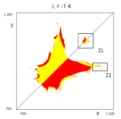
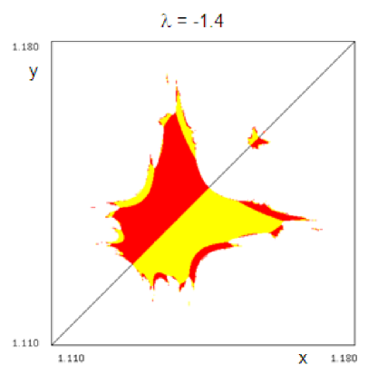
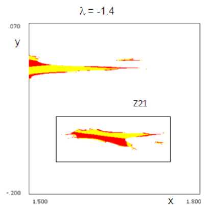
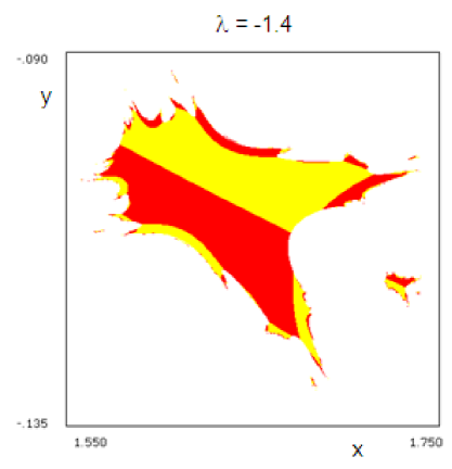
Figures 1-4 show the basin of two coexisting attractors and successive enlargements in the case of the map , each attractor being an order 2 cycle: one basin is in yellow, the other one in red. Basins are symmetrical, non-connected and fractal. Successive enlargements of the 2-dimensional phase space on the diagonal (Z1 area) and on Z2 area show auto-similarity properties. The shape of each enlarged piece of basin is similar to the precedent piece with an alternation between the successive locations of symmetrical yellow and red basins. Such a shape can be explained by using the critical manifolds of (1) [4, 5].
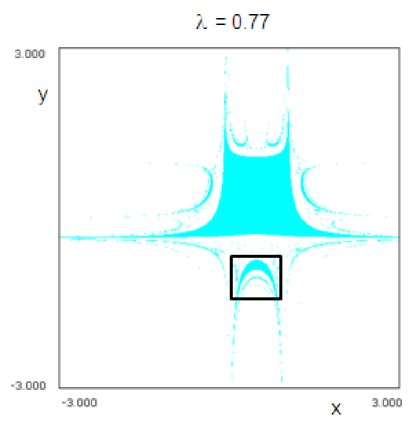
Figures 5-6 show the fractal basin of a fixed point for the map . This basin is non-connected. Figure 6 shows clearly the auto-similarity property. The appearance of such a fractal basin can also be explained by using the critical manifolds [4, 7].
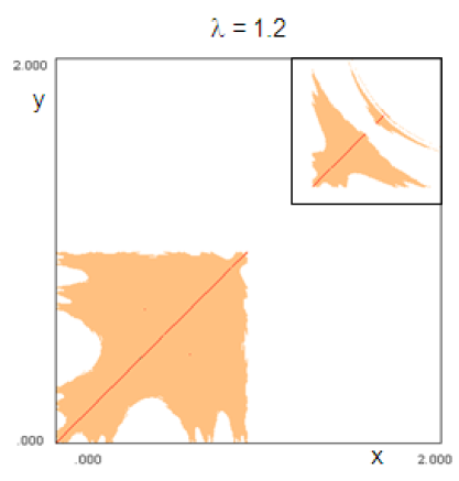
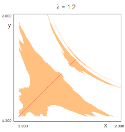
Figures 7-8 show a fractal basin for the map . The attractor is chaotic and it is not represented on the Figures [8]. As in the case of the map (1), the successive auto-similar pieces of the basin are located on the diagonal. The fractalization of the basins can be understood by means of the critical manifolds [4, 8], as in the case of the maps (1) and (2).
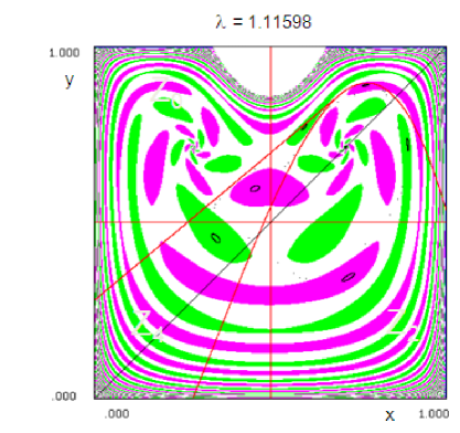
4 Multistability and Fractal boundaries
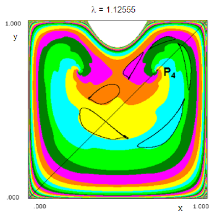
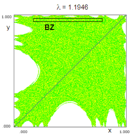
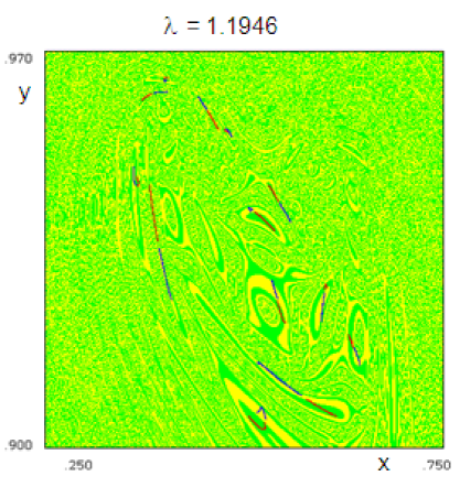
Multistability among several attractors is very frequent in these models. As it can be seen in the Figures 9-12, the basins can take complex and fractal forms. Figure 9 shows the shape of the basins of three different attractors. The boundary among those basins is fractal, due to the accumulation and the entanglement close to the boundary of the square . Figure 10 represents the basin of two different attractors, wich are order 3 invariant closed curve (ICC), for the map . Then we obtain six different basins in for each piece of the two co-existing order 3 ICC in . Some of the basins can be riddled, that is, successive zooms of a basin zone cannot differentiate the boundaries between the basins of the different attractors. Such basins are shown on Figures 11-12. There are two chaotic attractors, which are order 52 chaotic rings. They are called weakly chaotic because of the greater Lyapunov exponent, which is slightly positive [7].
References
- [1] Lopez-Ruiz R., Fournier-Prunaret D., Logistic Models for Symbiosis, Predator-prey and Competition, Encyc. of Networked and Virtual Organizations, vol. II (2008) 838–847.
- [2] Cushing J.M., Levarge S., Chitnis N., Henson S.M., Some discrete competition models and the Competitive Exclusion Principle, J. Diff. Eqns. Appl., vol. 10 (2004) 1139–1151.
- [3] Lopez-Ruiz R., Perez-Garcia C., Dynamics of two logistic maps with a multiplicative coupling, Int. J. Bif. Chaos, vol. 2 (1992) 421–425.
- [4] Mira C., Fournier-Prunaret D., Gardini L., Kawakami H., Cathala J.C., Basin bifurcations of 2-dimensional noninvertible maps. Fractalization of basins, Int. J. Bif. Chaos, vol. 4 (1994) 343–381.