Formation of caustics in Dirac-Born-Infeld type scalar field systems

Abstract

We investigate the formation of caustics in the Dirac-Born-Infeld type scalar field systems for generic classes of potentials, viz., massive rolling scalar with potential, $V(\phi)=V_{0}e^{\pm\frac{1}{2}M^{2}\phi^{2}}$ and inverse power-law potentials with $V(\phi)=V_{0}/\phi^{n},~{}0<n<2$. It is found that in the case of exponentially decreasing rolling massive scalar field potential, there are multi-valued regions and regions of likely to be caustics in the field configuration. However there are no caustics in the case of exponentially increasing potential. We show that the formation of caustics is inevitable for the inverse power-law potentials under consideration in Minkowski space time whereas caustics do not form in this case in the FRW universe.

I Introduction

The discovery of the late time accelerated expansion of universe is one of the most surprising findings in modern cosmologyRiess and posses a serious challenge to fundamental theories of physics. The resolution of cosmic acceleration riddle similar to the phenomenon of black body radiation might unveil new secrets of nature.

It is now widely believed that the late time acceleration of universe is due to an exotic form of energy with large negative pressure known as dark energy which is the dominant fraction of the energy content of present universe review1 ; review2 ; review3 . The simplest dark energy model based upon cosmological constant is faced with fine tuning problem of an acceptable level. As an alternative to cosmological constant, a variety of scalar field models is proposed in recent years to provide a viable explanation for the phenomenon of late time cosmic acceleration Zlatev ; Armendariz ; Kamenshchik ; Padmanabhan ; Garousi . Though the scalar field models have limited predictive power but nevertheless can be of interest in case they can exhibit some generic features allowing to alleviate the fine tuning and coincidence problems or could be motivated from a fundamental theory of high energy physics. The Dirac-Born-Infeld (DBI) scalar field model is string inspired and certainly invites attentionsen . Unlike generic quintessence models with tracker solutions, there exists no solution which can mimic scaling matter/radiation regime in case of the tachyon field samicop ; samiothers ; allthat ; Paddy ; staro ; Bagla ; AF ; AL ; GZ . These models necessarily belong to the class of thawing models: At early times, the expansion dynamics is governed by the background fluid whereas the tachyon field remains subdominant and frozen. However, as the background energy density redshifts and becomes comparable to the field energy density, the field begins to evolve and subsequently overtakes the background to become the dominant component of universe.

Tachyon models do admit scaling solution in presence of a hypothetical barotropic fluid with negative equation of state. Tachyon fields can be classified by the asymptotic behavior of their potentials for large values of the field: (i) $V(\phi)\to 0$ faster than $1/\phi^{2}$ for $\phi\to\infty$. In this case dark matter like solution is a late time attractor. Dark energy may arise in this case as a transient phenomenon. (ii) $V(\phi)\to 0$ slower than $1/\phi^{2}$ for $\phi\to\infty$ ; these models give rise to dark energy as late time attractor. The two classes are separated by $V(\phi)\sim 1/\phi^{2}$ which is a scaling potential with $w({\phi})=constant$. The present state of observations does not allow to distinguish amongst various scalar field models and leaves the dark energy metamorphosis as a future challenge for observational cosmology.

The formation of caustics in field profile in the mass free space is an undesirable consequence in the field theoretical models in cosmology as it indicates the failure of physical theories to explain the evolution of field in that particular region. Thus the study of formation of caustics in the field configuration is one of the best techniques to investigate the fundamental shortcoming of the field theory for a specific potential.

Inspite of the exiting features of cosmological dynamics based upon DBI scalars, it might happen that these models lead to formation of caustics where the second and the higher-order derivatives of the field become singular. As demonstrated in Ref. staro , caustics inevitably form in tachyon system with potentials decaying faster than $\phi^{-2}$ at infinity. We do not know whether caustics are generic prediction of string theory or appear as a result of the derivative truncation leading to the DBI action. It remains to extend the analysis of Ref. staro to the case of inverse power law potentials, $V\sim\phi^{-n}$ with $0<n<2$ analysed in Ref. Copeland . Caustics normally form in systems with pressureless dust which is mimicked by tachyon field with run away potentials. It is therefore quite likely that caustics may not develop in Born-Infeld systems with a ground state at a finite value of the field. The rolling massive scalar potential, $V(\phi)=V_{0}e^{\frac{1}{2}M^{2}\phi^{2}}$ belongs to this category.

In this paper, we address the issue of caustic formation for DBI scalar field systems for inverse power potentials giving rise to dark energy as a late time attractor and the massive rolling scalar. In the section II, we present the DBI type general scalar field equation for the 1 + 1 flat space time and review the formalism of field dynamics related to caustic formation based upon Ref. staro . We also extend the analysis to the case of isotopic and homogeneous expanding universe to see the formation of caustics in the field in more real situation. In section III, we discuss our numerical results. To have a comprehensive view of the scalar field pattern, the general field equations are solved numerically as well analytically in the homogeneous and inhomogeneous situations for the two different classes of field potentials mentioned above. For the inhomogeneous case, we solve the evolution equations analytically using the method of characteristics staro to check the formation of caustics in the field profile using the geometrical interpretation of the solution. Main results of our analysis are summarized in the last section.

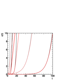
Figure 1: The numerical solution of the equation (26) (red line) and the analytic solution of equation (27) (black line) for different values of $M$ and $\phi_{0}$. The solid line is for the initial value of field $\phi_{0}$ = 0.001 and the dotted line is for $\phi_{0}=0.1$. Three different sets are due to three different values of $M$ = 1, 0.5 and 0.1 along the increasing values of t. The discrepancy between these two solutions is obvious after some initial period depending upon the values of $M$ and $\phi_{0}$.

II The Dirac-Born-Infeld type scalar field system

The DBI type action for a scalar field $\phi$, referred to as tachyon field hereafter, is given by sen ; staro ; review2 ,

$$S=-\int d^{4}x\sqrt{-g}~{}V(\phi)\sqrt{1+{\partial_{\mu}\phi\partial^{\mu}\phi}}~{},$$ (1)

where $V(\phi)$ is the potential of the field $\phi$. The field equation derived from the action (1) is,

$$\nabla_{\mu}\nabla^{\mu}\phi-\frac{\nabla_{\mu}\nabla_{\mu}\phi}{1+\nabla_{\alpha}\phi\nabla^{\alpha}\phi}\nabla^{\mu}\phi\nabla^{\nu}\phi-\frac{V_{,\phi}(\phi)}{V(\phi)}=0,$$ (2)

where the covariant derivative of the field $\phi$ with respect to the metric $g_{\mu\nu}$ is denoted by $\nabla_{\mu}$.

II.1 Minkowski 1+1 dimensional analysis

In what follows, we shall first consider the field equations in 1 + 1 dimensional Minkowski space. Caustics formation can easily be analysed in this case. If caustics do not form in Minkowski space time, we would expect the result to hold in the expanding universe as expansion should work against the formation of caustics. However, in the opposite case, it essential to incorporate expansion to reach the final conclusion.

In this case, the equation (2) takes the form,

$$\ddot{\phi}=\left(1+\phi^{\prime 2}\right)^{-1}\left[\left(1-\dot{\phi}^{2}+\phi^{\prime 2}\right)\left(\phi^{\prime\prime}-\frac{V_{,\phi}(\phi)}{V(\phi)}\right)+2\phi^{\prime}\dot{\phi}\dot{\phi}^{\prime}-\phi^{\prime 2}\phi^{\prime\prime}\right].$$ (3)

Here the time and space derivatives of the field $\phi$ are indicated by the dot and prime over $\phi$ respectively.

In order to understand the time and space evolution of the field $\phi$ in 1 + 1 dimension under a specific field potential, let us first consider some general aspects related to the equation (3) for the homogeneous and inhomogeneous fields.

If the scalar field is homogeneous, then $\phi^{\prime}=0$, and hence the equation (3) for such a field simplifies to,

$$\frac{\ddot{\phi}}{1-\dot{\phi}^{2}}+\frac{V_{,\phi}(\phi)}{V(\phi)}=0.$$ (4)

For a particular potential, the time evolution of the homogeneous field can be obtained from this equation (4). In the case of an inhomogeneous scalar field, $\phi^{\prime}$, $\phi^{\prime\prime}>0$, however they should be sufficiently less then unity for a realistic scalar field in cosmology staro . Under this condition, the equation (3) can be written as,

$$\ddot{\phi}=\left(1-\dot{\phi}^{2}+\phi^{\prime 2}\right)\left(\phi^{\prime\prime}-\frac{V_{,\phi}(\phi)}{V(\phi)}\right)=P(\phi)Q(\phi),$$ (5)

where,

$$\begin{split}P(\phi)=1-\dot{\phi}^{2}+\phi^{\prime 2}.\\ Q(\phi)=\phi^{\prime\prime}-\frac{V_{,\phi}(\phi)}{V(\phi)}.\end{split}$$ (6)

The equation of $P(\phi)$ contains both the time and space derivatives of the field and therefore this parameter can be used as an indicator of the pattern of evolution of the field governed by the particular field potential. For example, if the field $\phi(x,t)$ rapidly approaches the configuration $P(\phi)=0$, it then indicates that the time and space evolution of the field is such that it rapidly approaches $\dot{\phi}^{2}-\phi^{\prime 2}=1$. Alternatively, we may say that, under this situation the field $\phi(x,t)$ is almost similar to some subsidiary field $\theta(x,t)$ whose time and space evolution is constrained by the equation staro ,

$$\dot{\theta}^{2}-\theta^{\prime 2}=1.$$ (7)

The field may approaches to the configuration $P(\phi)=0$ from both directions, viz. from above or below zero, depending upon the initial state of the field. If the initial state of the field is such that initially $P(\phi)>0$, then $P(\phi)$ will asymptotically approach to zero from above, otherwise it will tend to be zero from below staro . Similarly, if $P(\phi)\approx 1$, it implies that, $\dot{\phi}^{2}\approx\phi^{\prime 2}$, i.e., the type of evolution of the field $\phi(x,t)$ with respect to space and time are nearly equal. In this case also, we may consider that the $\phi(x,t)$ is almost similar to some subsidiary field $\omega(x,t)$ whose time and space variations are related by the equation,

$$\dot{\omega}^{2}-\omega^{\prime 2}=0.$$ (8)

The extensive numerical solutions of the equation (5) for the scalar field with the two different classes of field potentials of our interest clearly showed the above behavior of $P(\phi)$. Thus the equation (5) has two attractors, one for $P(\phi)=0$ and the other for $P(\phi)=1$, depending on the field potential and hence $P(\phi)$ can be used to define the following relation,

$$\dot{\phi}=\sqrt{1+\phi^{\prime 2}-P(\phi)}.$$ (9)

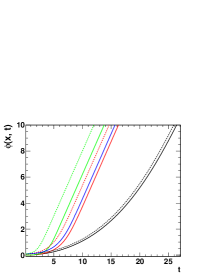
Figure 2: The numerical solutions of the equation (29) for different values of $M$ and $\phi_{0}$. Black, red and green lines are for $M$ = 0.1, 0.5 and 1 respectively. The solid line represents $\phi_{0}$ = 0 and the dotted line $\phi_{0}$ = 0.1. For all these plots we consider $\phi^{\prime}$ = 0.01 and $\phi^{\prime\prime}$ = 0.02. The blue line represents the solution with $\phi_{0}$ = 0, $M$ = 0.5, $\phi^{\prime}$ = 0.002 and $\phi^{\prime\prime}$ = 0.001. For all cases time variation of the field is very slow initially and then it increases rapidly as time passages.

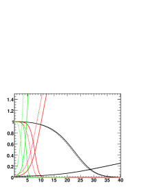
Figure 3: The variation patterns of $P(\phi)$ and $Q(\phi)$ with respect to time for the potential (25) corresponding to the initial conditions of the figure 2. The falling lines are for $P(\phi)$ and raising lines are for $Q(\phi)$. The overall pattern are same for all initial conditions.

If we consider that the scalar field $\phi(x,t)$ itself satisfies the subsidiary field equations (7) and (8) under different conditions, then analytic solutions of these two equations correspond to free relativistic massive wave propagation along the characteristics of the field $\phi(x,t)$. From the particle point of view, equations (7) and (8) can be viewed as the dynamical descriptions of the motion of free massive particle under different situations. From this point of view, the trajectories $x(t,q)$, (where $q$ is the initial spatial coordinate of the field, i. e. $x(0,q)=q$) of individual particles and the corresponding evolution of the field configuration can be obtain from the parameterized solutions of the characteristic equations of two variables, viz., $q$ and the affine parameter $s$ along each curve, which are given by staro ,

$$\frac{dx}{ds}(q,s)=P,\phi^{\prime}=2\phi^{\prime};\;\;x(q,0)=q.$$ (10)

$$\frac{dt}{ds}(q,s)=P,\dot{\phi}=-2\dot{\phi};\;\;t(q,0)=0.$$ (11)

$$\frac{d\phi}{ds}(q,s)=\phi^{\prime}P,\phi^{\prime}+\dot{\phi}P,\dot{\phi}=2\phi^{\prime 2}-2\dot{\phi^{2}};\;\;\phi(q,0)=\phi_{i}(q).$$ (12)

Solving these equations and using equation (9) we may write,

$$x(q,s)=q+2s\phi_{i,q}.$$ (13)

$$t(q,s)=-2s\sqrt{1+\phi_{i,q}^{2}-P(\phi)}.$$ (14)

$$\phi(q,s)=\phi_{i}(q),\;\mbox{for}\;P(\phi)=1\;\;\mbox{and}\;\phi(q,s)=\phi_{i}(q)-2s,\;\mbox{for}\;P(\phi)=0.$$ (15)

Where $\phi_{i,q}=\phi^{\prime}(q,s)$. Eliminating the affine parameter $s$ from the above equations, we obtain the parametric solution for the field $\phi(x,t)$ as,

$$x(q,t)=q-\frac{\phi_{i,q}}{\sqrt{1+\phi_{i,q}^{2}-P(\phi)}}t.$$ (16)

$$\phi(q,t)=\phi_{i}(q),\;\mbox{for}\;P(\phi)=1\;\mbox{and}\;\phi(q,t)=\phi_{i}(q)+\frac{t}{\sqrt{1+\phi_{i,q}^{2}}},\;\mbox{for}\;P(\phi)=0.$$ (17)

The equation (16) will provide us the trajectories of the free massive particles in the field and the equation (17) will give us the pattern of evolution of the field with respect to time staro . Hence these two equations will give us the geometrical form to see the formation of caustics in the field profile and the evolution of the field configuration with any presumed initial field profile under a specific field potential. In what follows, we shall consider the potentials of our interest for the specific solutions of the equations (4) and (5). Although our main interest is the solution of equation (5), for the completeness of the picture we present the solution of equation (4) also. From the solutions of equation (5) for the following three different field potentials, we shall obtain the characteristics curves from equation (16) which will show clearly whether there are caustics in the field configuration.

II.2 Generalization to the case of expanding universe

So far, for simplicity we have considered the field in 1 + 1 dimensional Minkowski space time. However for the real cosmological applications, it is necessary to consider the field in 3 + 1 dimensions in the expanding universe. It should be noted that the extension of the field from 1 + 1 dimension to the 3 + 1 dimensions is a matter of analogical enhancement of the one dimensional spatial coordinate to the three dimensional spatial coordinates. Hence the basic form of all equations discussed above will remain same in 3 + 1 dimensions, also except that the space derivative has to be replaced by the nabla operator $\nabla$, and the spatial coordinates $x$ and $q$ by the vectors ${\bf{r}}$ and ${\bf{q}}$ respectively in the relevant equations. Similarly if we take a spatially flat Friedmann-Robertson-Walker (FRW) metric with a scale factor $a(t)$, then equation for the scalar field $\phi$ in an expanding universe can be obtain from the equation (2) as,

$$\frac{\ddot{\phi}}{1-\dot{\phi}^{2}}+3H\dot{\phi}+\frac{V_{,\phi}(\phi)}{V(\phi)}=0,$$ (18)

where $H=\dot{a}/a$ is the Hubble rate and can be expressed in the scalar field dominated expanding universe as,

$$H^{2}=\frac{8\pi G}{3}\frac{V(\phi)}{\sqrt{1-\dot{\phi}^{2}}}.$$ (19)

The equation (18) is equivalent to the equation (4) of 1 + 1 dimension. If some small inhomogeneous perturbations arise in the scalar field of the expanding universe, then these perturbations will generate the small perturbations in the FRW metric which can be expressed by the Newtonian gravitational potential $\Phi_{G}(t,{\bf r})$ as staro ; staro1 ,

$$ds^{2}=-(1+2\Phi_{G})dt^{2}+(1-2\Phi_{G})a^{2}(t)dr^{2},$$ (20)

where we have use the metric convention as $(-,+,+,+)$. If for a particular potential of the scalar field of expanding universe with small inhomogeneous field perturbations lead to the state of the field as in the cases of the equations (7) and (8) of the 1 + 1 dimension, then the corresponding equations for the field $\phi$ itself of the expanding universe represented by the metric equation (20) are given by staro ,

$$\dot{\phi}^{2}-\frac{1}{a^{2}}(\nabla\phi)^{2}=1+2\Phi_{G}.$$ (21)

$$\dot{\phi}^{2}-\frac{1}{a^{2}}(\nabla\phi)^{2}=0.$$ (22)

If we solve these two equations by the method of characteristics as in the case of 1 + 1 dimension the corresponding equations of (16) and (17) would be,

$${\bf r}({\bf q},t)={\bf q}-\frac{1}{a^{2}}\frac{(\nabla_{\bf q}\phi)t}{\sqrt{1+\frac{1}{a^{2}}(\nabla_{\bf q}\phi)^{2}+2\Phi_{G}}},\;\mbox{for}\;P(\phi)=0\;\mbox{and}\;{\bf r}({\bf q},t)={\bf q}-\frac{t}{a},\;\mbox{for}\;P(\phi)=1.$$ (23)

$$\phi({\bf q},t)=\phi_{i}({\bf q})+\frac{(1+2\Phi_{G})t}{\sqrt{1+\frac{1}{a^{2}}(\nabla_{\bf q}\phi)^{2}+2\Phi_{G}}},\;\mbox{for}\;P(\phi)=0\;\mbox{and}\;\phi({\bf q},t)=\phi_{i}({\bf q}),\;\mbox{for}\;P(\phi)=1.$$ (24)

The scale factor $a(t)$ assumes different forms at different stages of the evolution of universe. For example, in radiation dominated stage, $a(t)=a_{0}t^{1/2}$ and in the scalar field dominated stage $a(t)=a_{0}t^{2/3}$ staro ; staro1 if the tachyon potential vanishes at infinity faster than $1/\phi^{2}$. In case of rolling massive scalar or the inverse power-law potentials $V(\phi)\sim 1/\phi^{n}$ with $0<n<2$ , dark energy is a late time attractor and the scale factor takes the form $a(t)=a_{0}t^{2/(3(1+w))}$ with suitable negative values of $w$. The fluctuations in the tachyon field grow lineally with time while the metric fluctuations remain constant for potentials decreasing faster than $1/\phi^{2}$ at infinitystaro ; staro1 . However, in case of rolling massive scalar and inverse power-law potentials with $0<n<2$ that would be of interest to us, both the fluctuations do not grow staro1 ; Garousi

III Caustic formation

In this section we apply the above formalism to investigate the possibility of caustic formation in the DBI tachyon system with two generic classes of potentials and present the results of numerical simulation.

III.1 Exponentially decreasing rolling massive potential

The exponentially decreasing rolling massive scalar field potential is given byCopeland ,

$$V(\phi)=V_{0}e^{-\frac{1}{2}M^{2}\phi^{2}},$$ (25)

where $V_{0}$ and $M$ are constants. For this potential the homogeneous scalar field equation (4) becomes,

$$\frac{\ddot{\phi}}{1-\dot{\phi}^{2}}-M^{2}\phi=0.$$ (26)

The numerical solution of this equation is shown in the figure 1 for different values of the arbitrary constant $M$ and initial values of field $\phi_{0}$. The values of $M$ chosen in this figure are 0.1, 0.5 and 1. On the other hand two values of $\phi_{0}$ are considered for this figure, which are 0.001 and 0.1. If the time variation of the scalar field is very slow, then we may consider that $\dot{\phi}<<1$. In this case, equation (26) further simplifies to,

$$\ddot{\phi}-M^{2}\phi=0.$$ (27)

The solution of this equation is trivial and can be written as,

$$\phi=\phi_{0}cosh(Mt),$$ (28)

where $\phi_{0}$ is the constant initial field value. The plots of this equation are also shown in the figure 1 for same values of $M$ and $\phi_{0}$ as for the above case to compare with the numerical solution. The red line indicates the numerical solution and black line indicates the analytic one. The solid line is for the initial field $\phi_{0}$ = 0.001 and the dotted line is for $\phi_{0}$ = 0.1. Three different sets are due to three different values of $M$ = 1, 0.5 and 0.1 along the increasing values of t. It is observed from the figure 1 that the assumption of very slow variation of the field with respect to time is correct only for some initial period that depends upon the values of $M$ and $\phi_{0}$. For low values $M$ and $\phi_{0}$ this period is longer than their higher values. As the time increases beyond this period, the discrepancy between the solutions of equations (26) and (27) increases rapidly. The overall trend of time variation of the field with different possible initial conditions is almost same, the only difference is that, this variation is slower for some initial period if the field is started with smaller values of $M$ and $\phi_{0}$ than their higher values.

The inhomogeneous scalar field equation(5) for this potential can be written as,

$$\ddot{\phi}=\left(1-\dot{\phi}^{2}+\phi^{\prime 2}\right)\left(\phi^{\prime\prime}+M^{2}\phi\right).$$ (29)

The numerical solutions of the equation (29) for the same values of $M$ as in the previous cases, but for $\phi_{0}$ = 0 and 0.1 are shown in the figure 2. In the figure the black line is for $M$ = 0.1, red line is for $M$ = 0.5 and green line for $M$ = 1. The solid line represents for $\phi_{0}$ = 0 and the dotted line for $\phi_{0}$ = 0.1. Since the solution of the inhomogeneous equation (29) depends upon the values of $\phi^{\prime}$ and $\phi^{\prime\prime}$, so for these plots in this figure we consider $\phi^{\prime}$ = 0.01 and $\phi^{\prime\prime}$ = 0.02. Moreover to check the dependency of the solution on $\phi^{\prime}$ and $\phi^{\prime\prime}$, we consider another set of values of these two parameters as 0.002 and 0.001 respectively together with $M$ = 0.5 and $\phi_{0}$ = 0.1. The result of this solution is shown in this figure by the blue line. We observe that for all cases the variation or the evolution of the field with time is very slow in the initial period based on the values of the $M$ and $\phi_{0}$, then it develops rapidly as time passages. For low values of $M$ and $\phi_{0}$ this initial period enhances slightly and the time variation is also relatively slower for such values. The value of $M$ has significant effect over the variation of the field with time than $\phi_{0}$ which is also noticed for the homogeneous case. Since this is an arbitrary parameter, we can assume any value of it for a solution, however its actual value can not be substantially small because for such a small value the time evolution of the field will halt for a considerable period of time. The $\phi^{\prime}$ and $\phi^{\prime\prime}$ does not have any effect on the time evolution of the field, whereas they only effect to shift the magnitude of field in the same direction of their magnitude variations (i.e. along the increasing or decreasing order). Thus for our remaining discussion, related to this field potential, we will not consider again the effect $\phi^{\prime}$ and $\phi^{\prime\prime}$ over the field.

The variations of $P(\phi)$ and $Q(\phi)$ with respect to time that are obtained from the numerical solutions for $\phi(x,t)$ are plotted in the figure 3. In this figure, the falling lines are for $P(\phi)$ and raising are for $Q(\phi)$. The color and style of the line represent the corresponding values of $M$ and $\phi_{0}$ as in the case of the figure 2. As mentioned earlier the state of the field with respect to time and space is indicated by the behavior of the $P(\phi)$ at the corresponding time. so, here we are mainly interested in $P(\phi)$ only.

From the pattern of variation of $P(\phi)$ with time we observed that during some initial period, which depends upon the value of $M$ and $\phi_{0}$, the value of $P(\phi)$ is $\approx 1$ and beyond this period its value falls rapidly to zero. The length of this initial period is more for lower values of $M$ and $\phi_{0}$ (effect is prominent for the parameter $M$ as mentioned earlier), otherwise the behaviour of time variation of $P(\phi)$ is similar for all initial conditions. To be more specific, we consider the solution of $P(\phi)$ with $M$ = 1 and $\phi_{0}$ = 0, and the initial field configuration as $\phi_{i}(q)=exp(-q^{2})$ staro , then we obtain the characteristic curves from equation (16) which are shown in the left panel of the figure 4.

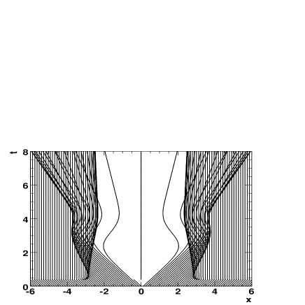
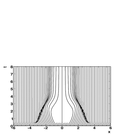
Figure 4: The particle trajectories in 1 + 1 Minkowski space obtain from equation (16) (left) and in FRW expanding universe obtain from equation (23) (right) with potential (25) and initial field profile $\phi_{i}(q)=exp(-q^{2})$. Both panels of figure are obtain with the initial condition $M$ = 1 and $\phi_{0}$ = 0.

From these characteristic curves it is interesting to note that there are likely to be caustics as well as multi-valued regions in the field profile. Apart from these, there are regions of twisting of the characteristic curves. The regions of caustics and multi-valued start at the points $x=\pm 3$. As the behaviour of the $P(\phi)$ is similar for all initial conditions mentioned above, therefore we will get the similar characteristic curves with caustics and multi-valued regions at different locations corresponding to the values of $M$ and $\phi_{0}$. Obviously for smaller values of $M$ and $\phi_{0}$ these location will shift to the higher value of t. But it is sure that there is no way to avoid these unphysical regions for any value of initial field parameters. Thus we may infer that the formation of caustics and multi-valued regions are independent of the initial conditions of the field.

The evolution of the field configuration $\phi(x,t)$ with $\phi_{i}(q)=exp(-q^{2})$ and for the same initial condition as in the case of characteristic curves are shown in the figure 5 at different times. It should be pointed out that to draw the field configuration at $t=5$ we consider that $P(\phi)=0$ (which is almost the case. Beyond this value of $t$, $P(\phi)$ is obviously zero). Within the period, when $P(\phi)$ falls from almost one to zero, field evolves very rapidly with time, which is not significant to be visualized geometrically. The same observation can be made for the evolution of the field configuration with different initial conditions and consequently with the different values of time after which $P(\phi)$ falls to zero.

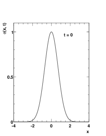
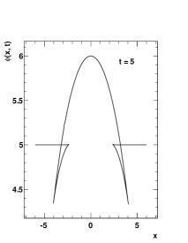
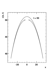
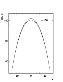
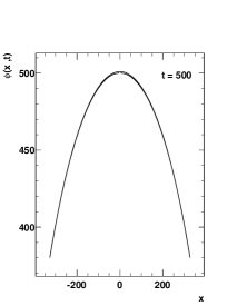
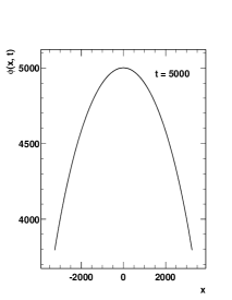
Figure 5: The evolution of the field configuration $\phi(x,t)$ with potential (25) and $\phi_{i}(q)=exp(-q^{2})$ at different times for the initial condition $M$ = 1 and $\phi_{0}$ = 0.

Heuristically speaking, expansion works against caustics formation. It is therefore necessary to investigate the corresponding situation in case of the expanding universe using equations (23) and (24). Without going into detail of the scalar field dynamics in the expanding universe under this potential, we assume that the field behaves in a manner equivalent to 1 + 1 dimensional case (which is specified by the behavior of $P(\phi)$). Since the average matter density of the universe is quite low to obtain a substantial value of the Newtonian gravitational potential $\Phi_{G}(t,{\bf r})$ Tren ; Lee of the universe, we shall neglect $\Phi_{G}$ in comparison to unity. Secondly, as dust like solution is a late attractor in the present case, we assume $a(t)\sim t^{2/3}$. Under these considerations, we obtain the characteristic curves from equation (23) with the initial field profile as mentioned above are shown in the right panel of the figure 4 for the one dimensional space. It is observed that the patterns of the characteristics curves are different in this case from the 1 + 1 dimensional Minkowski space time and the caustics are more distinctly formed in the field profile if the field behave in a similar manner as in the 1 + 1 dimension with this exponentially decreasing rolling massive potential. From the numerical calculations under the above considerations we found that the evolution patterns of the field obtained from the equation (24) remain nearly same as its initial profile. We should note that the field rolls slowly for a short while near the origin but quickly enters the fast roll to mimic dark matter like regime described by $a(t)\sim t^{2/3}$. Using equations (18) and (19), we have verified that situation depicted in figure 4 does not change if the detailed field dynamics is taken into account.

III.2 Exponentially increasing rolling massive potential

Now we consider rolling massive scalar potential $V(\phi)$ given by Copeland ; Sami ,

$$V(\phi)=V_{0}e^{\frac{1}{2}M^{2}\phi^{2}},$$ (30)

In this case, the homogeneous field equation (4) can be written as,

$$\frac{\ddot{\phi}}{1-\dot{\phi}^{2}}+M^{2}\phi=0.$$ (31)

The numerical solutions of this equation is shown in the figure 6 by dotted line with three different colors for three different values of $M$ as in case of previous potential, viz., black for 0.1, red for 0.5 and green for 1. The upper set is for $\phi_{0}$ = 1 and lower set is for $\phi_{0}$ = 0.5. The field $\phi$ for this potential is oscillatory in nature.

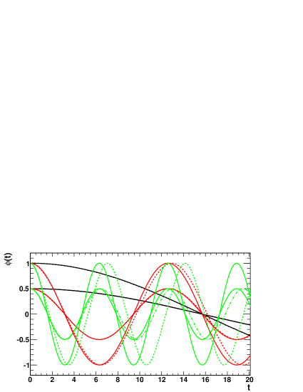
Figure 6: The numerical solutions of the equation (31) (dotted line) and the solutions of equation (32) (solid line) for three different values of $M$ = 0.1, 0.5 and 1, which are represented by black, red and green colors respectively. The upper set is for $\phi_{0}$ = 1 and lower set is for $\phi_{0}$ = 0.5. There is a good agreement between the numerical and analytic solutions although there is gradual phase shift between them as time passages depending on the values of $M$ and $\phi_{0}$.

Since $\phi$ is oscillatory just like a simple harmonic motion and its obvious equation can be obtain by considering $\dot{\phi}<<1$, which is in this case is,

$$\ddot{\phi}+M^{2}\phi=0,$$ (32)

and the nature of $\phi$ is the solution of this equation,

$$\phi=\phi_{0}cos(Mt),$$ (33)

where $\phi_{0}$ is a constant, the field amplitude. The solution (33) are presented in the figure 6 for same values of $M$ and $\phi_{0}$ as described above. It is seen that the solutions of equations (31) and (32) are in good agreement, however there is gradual phase shift between them because the second solution is due to slow variation of $\phi$. The rate of this phase shift depends upon the values of $M$ and $\phi_{0}$, which is slower for the smaller values of these two initial field parameters. On the other hand, the time period of oscillation of the field depends on these two parameters in the opposite way, i. e. the time period increases with decreasing values of them. As in the case of the previous potential, in this case also the effect of $M$ on the field is more prominent than $\phi_{0}$. The amplitude of oscillation solely depends on the value of $\phi_{0}$ as it is clear from the figure.

The inhomogeneous scalar field equation (5) in this case can be written as,

$$\ddot{\phi}=\left(1-\dot{\phi}^{2}+\phi^{\prime 2}\right)\left(\phi^{\prime\prime}-M^{2}\phi\right).$$ (34)

The numerical solutions of the equation (34) with $\phi^{\prime}=0.01$, $\phi^{\prime\prime}=0.02$ and with three different values of $M$ same as above, and $\phi_{0}$ = 0, 0.1 are shown in the figure 7. The three colors corresponds to the respective values of $M$ as mentioned above for the homogeneous case. Here the solid line indicates the solution for $\phi_{0}$ = 0, whereas the dotted line for the $\phi_{0}$ = 0.1. To understand the effect of $\phi^{\prime}$ and $\phi^{\prime\prime}$ on the inhomogeneous field for this potential we consider the solution of the equation (34) with the set of initial field values as $\phi^{\prime}$ = 0.002, $\phi^{\prime\prime}$ = 0.001, $M$ = 0.1 and $\phi_{0}$ = 0, which is shown by the blue line in the figure. We have seen that the inhomogeneous field is also oscillatory in nature, time period of which depends upon the values of $M$ and $\phi_{0}$ in the same way as in the homogeneous case, however the small value of $M$ effects significantly on both time period and amplitude of oscillation. It should be noted that, the amplitude decreases for higher value of $\phi_{0}$ as $M$ decreases and there is a phase shift between oscillation patterns of field for different values of $\phi_{0}$, which decreases with decreasing value of $M$. The effect of $\phi^{\prime}$ and $\phi^{\prime\prime}$ on the field is only on the amplitude of its oscillation and we have seen that the amplitude decreases substantially for the lower value of space variation of the field. So the role of space variation factor is significant for this potential to avoid the unwanted large fluctuation or oscillation of the field for lower value of $M$. It also implies that in reality the space variation of the field should be sufficiently less that unity as previously mentioned.

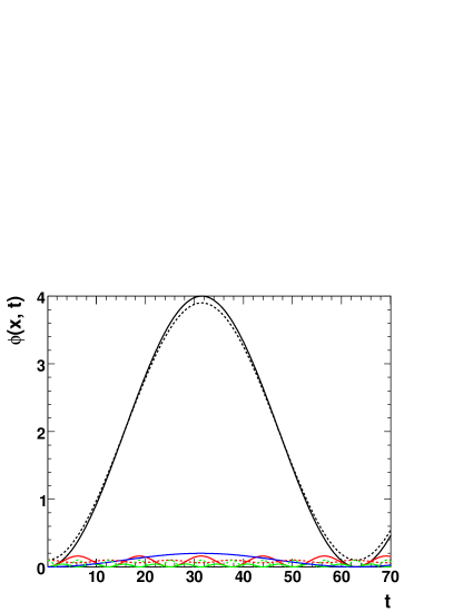
Figure 7: The numerical solutions of the equation (34) for different values of $M$, $\phi_{0}$, $\phi^{\prime}$ and $\phi^{\prime\prime}$. The line colors black, red and green are for $M$ = 0.1, 0.5 and 1 respectively. Solid line refer to $\phi_{0}$ = 0 and dotted to $\phi_{0}$ = 0.1. All these plots are drawn for solutions with $\phi^{\prime}$ = 0.01 and $\phi^{\prime\prime}$ = 0.02. The blue line indicates the solution with $M$ = 0.1, $\phi_{0}$ = 0, $\phi^{\prime}$ = 0.002 and $\phi^{\prime\prime}$ = 0.001.

The time variations of $P(\phi)$ and $Q(\phi)$ corresponding to above solutions of equation (34) are shown in the figure 8.

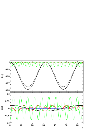
Figure 8: The time variation patterns of $P(\phi)$ and $Q(\phi)$ for the potential (30) corresponding to the solutions of equation (34) shown in the figure 7.

The values of $P(\phi)$ oscillates with time near unity from below with different amplitudes corresponding to the situations described above for the solutions of equation (34). For the value of $M$ = 0.1 the amplitude of oscillation of values of $P(\phi)$ is noticeably away from unity in comparison to other higher values of $M$ if we consider the value of $\phi^{\prime}$ = 0.01 and $\phi^{\prime\prime}$ = 0.02. So for further lower values of $M$ the amplitude of oscillation should move far away from unity. On the other hand if we consider the value $\phi^{\prime}$ = 0.002 and $\phi^{\prime\prime}$ = 0.001 for the same value of $M$ (i.e. 0.1), the oscillation of the values of $P(\phi)$ is negligible and its values are almost unity for all times. But intuitively enough, we may argue that the value of space variation of the field can not be very small beyond some limit as that will nullify the inhomogeneity condition of the field and similarly the value $M$ also can not be very small because then field will not be sustainable one for very large amplitude of oscillation. Hence for the real situation the value of $M$ and the space variation of the field should be such that oscillation of the field must be negligible. Under such considerations and for our present values of $M$ we may take on average the value of $P(\phi)$ as unity for all times. For the initial field configuration $\phi_{i}(q)=exp(-q^{2})$ as in the previous cases and $P(\phi)=1$, the characteristic curves for equation (16) are shown in the left panel of the figure 9.

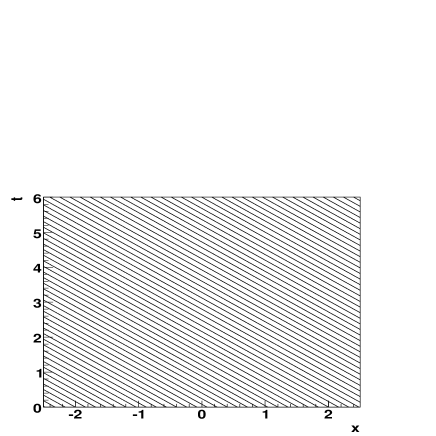
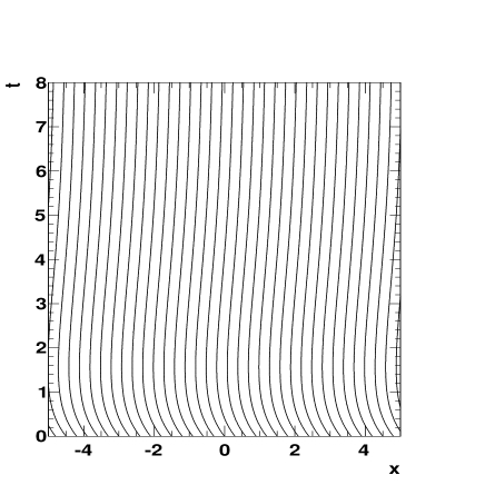
Figure 9: The particle trajectories in 1 + 1 Minkowski space obtain from equation (16) (left) and in FRW expanding universe obtain from equation (23) (right) with potential (30) and $\phi_{i}(q)=exp(-q^{2})$. The figure in the right panel is obtained from the numerical solutions of equations (18) and (19) of FRW expanding universe with the given potential for one spatial dimension taking constants $k=8\pi G$, $V_{0}$, $M$ as unity and the initial field value $\phi_{0}$ = 0.1.

It is clear from the panel of the figure that there are no caustics and there are no multivalued regions in the field configuration. This happens due to the almost steady nature of the field (because the average value of the field with time is a constant as clear from our argument together with the figure 7) and therefore the evolution pattern of the field for all times in this case will be same as in the previous case for $t=0$, i. e. same as the initial configuration of the field. As expansion works against caustics formation, we should not encounter caustics if expansion of universe is incorporated. Indeed, we have numerically checked that there are no caustics in the field profile in the expanding universe in this case, see the right panel of the figure 9.

III.3 Inverse power-law potentials

Finally we consider the inverse power-law potential of the form, given by Copeland ; Sami ,

$$V(\phi)=V_{0}\phi^{-n},~{}~{}0<n<2.$$ (35)

The late time accelerated expansion of the universe corresponds to $0\leq n\leq 2$ Abramo ; Copeland , and accordingly we restrict the value of the exponent $n$ within this range for our work.

We shall first restrict our attention to 1+1 dimensional Minkowski space time. In this case, the homogeneous field equation (4) is given by,

$$\frac{\ddot{\phi}}{1-\dot{\phi}^{2}}-\frac{n}{\phi}=0.$$ (36)

The numerical solutions of this equation is shown in the left panel of the figure 10 for $n=0.5,\;1.0\;\mbox{and}\;1.5$ with $\phi_{0}$ = 1. The difference of the solutions decreases for the higher values of $n$ as it is clear from the figure.

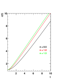
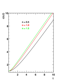
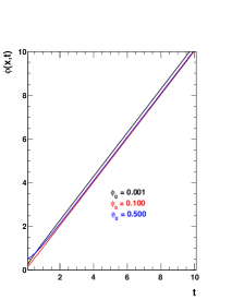
Figure 10: The numerical solutions of the homogeneous field equation (36) (left) and the inhomogeneous field equation (37) (middle) with $\phi_{0}$ = 1. The difference between the homogeneous and inhomogeneous solutions is insignificant. The right panel shows the three different solutions of the inhomogeneous equation for three different values of $\phi_{0}$ and for $n$ = 1. This panel clearly verifies that the time evolution of the field is almost independent of the initial value of the field for the inverse power-law potentials.

The inhomogeneous scalar field equation (5) in this case will take the form,

$$\ddot{\phi}=\left(1-\dot{\phi}^{2}+\phi^{\prime 2}\right)\left(\phi^{\prime\prime}+\frac{n}{\phi}\right).$$ (37)

The numerical solutions of the equation (37) with $\phi^{\prime}=0.01$, $\phi^{\prime\prime}=0.02$ and for $n=0.5,\;1.0,\;1.5$ with $\phi_{0}$ = 1 are shown in the middle panel of the figure 10. It should be noted that there is no significant difference between the solutions of homogeneous and inhomogeneous field equations for this inverse power-law potential, because the time variation of the field is more prominent than the space variation we have considered, which indeed should be for a mass free space. Moreover the field evolution pattern is almost independent of the initial condition of the field. However it has little impact on the magnitude of the field as time passage in a arbitrary manner as it is seen from the right panel of this figure. So the value of $\phi_{0}$ would be immaterial for the testing of the caustic formation in the field for the inverse power-law potentials. However we take care of the effect of $\phi_{0}$ on the variation $P(\phi)$ to see the way of rolling of its values with time which will be clear from the following discussion. The time variations of $P(\phi)$ and $Q(\phi)$ corresponding to the solutions of $\phi(x,t)$ as shown in the middle and the right panel of the figure 10 are shown in the figure 11.

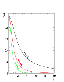
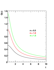
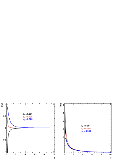
Figure 11: The time variation patterns of $P(\phi)$ and $Q(\phi)$ corresponding to the solutions shown in the middle and the right panels of the figure 10.

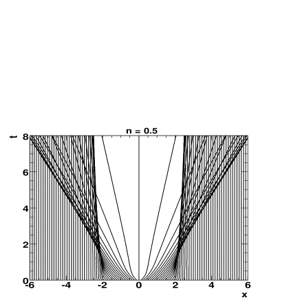
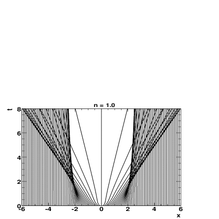
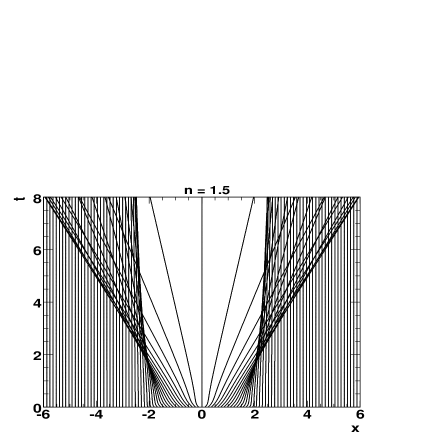
Figure 12: The particle trajectories in 1 + 1 Minkowski space obtain from equation (16) with potential (35) and $\phi_{i}(q)=exp(-q^{2})$ corresponding to the solutions of the equation (37) with $\phi_{0}$ = 1 as shown in the middle panel of the figure 10. Caustics and multi-valued regions are clearly formed in the space.

From the figure 11 we observed that values $P(\phi)$ for all $n$ rapidly falls to zero from above if the initial value of the field $\phi_{0}$ is not very small. It is interesting to note that, when the value of $\phi_{0}$ is very small, $P(\phi)$ falls rapidly to zero from below as indicated by the third panel of the figure 11. Notwithstanding, for all cases the value of $P(\phi)$ rolls to zero very fast (rate is more for lower value of $\phi_{0}$) as time passage and hence considering the initial field configuration as in the previous cases, the plots of the characteristic curves for equation (16) are shown in the figure 12 for $n=0.5,\;1.0\;\mbox{and}\;1.5$ with $\phi_{0}$ = 1.

The figure 12 vividly shows the formation of caustics and multi-valued regions in this case. It should be noted that the regions of caustics are not steady but slowly moves with time as the exponent $n$ of the potential increases. Due to pattern of variation of $P(\phi)$, we get the similar pattern of variation of field configuration at different times as in the case of exponentially decreasing rolling massive potential as shown in the figure 5.

As noted earlier, expansion works against caustic formation. The effect might become dramatic in case of inverse power-law potential under consideration with dark energy as late attractor. Thus the observed caustic formation in case of potential (35) may quite be the artifact of Minkowski space time. In order to reach the final conclusion in this regard, it is essential to incorporate the expansion of universe. The numerical solutions of evolution equations (18) and (19) are depicted in the figure 13 for all potentials, which are obtained by taking constants $k=8\pi G$, $V_{0}$, $M$, $n$ as unity and the initial field value $\phi_{0}$ = 0.1. The left panel provide us the evolution history of the scale factor $a(t)$ and right panel shows the variation of the equation state parameter $w$ of the field with time for all three potentials. It is clearly observed that, the time evolution of the scale factor is faster in the case of exponentially increasing massive potential than the inverse power-law potential. On the other hand in case of exponentially decreasing massive potential the scale factor becomes infinity after some initial period. The field is rolling faster to attain steady values in the case of the exponentially increasing and decreasing field potentials. Whereas in the case of the inverse power-law potential ($0<n<2$, the plot is shown for $n=1$) the field is evolving very slowly with time after some very brief initial period during which it evolves relatively fast. Though both the models (i. e. exponentially increasing and inverse power-law) can account for late time acceleration, the rolling massive scalar requires enormous fine tuning in order to be consistent with observation.

Since dark energy is late time attractor in the present case, we first for simplicity and consistency with the full solution of $a(t)$ as mentioned above, assumed that $a\sim t^{2/3(1+w)}$, incorporating all time dark energy effect in the scale factor. Now for the case of the scalar field in expanding universe with the inverse power-law potentials under the above mentioned assumptions and with this value of the scale factor for $w$ = - 0.9, we obtain the characteristic curves of the field given by the equation (23) look like as shown in the left panel of the figure 14. It is interesting to note that there are no caustics and multivalued regions in the field profile of dark energy dominated universe in contrast to the situation of 1 + 1 dimensional Minkowski space. Finally at this stage we intend to incorporate the dynamics exactly by taking the numerical solutions of equations (18) and (19). The numerical data of the scale factor $a(t)$ (see, figure 13) can then be used to solve the equation (23) to see the formation of caustics in the field profile for the given potential. The result of solution of this equation (23), i. e. the characteristic curves obtained by using the numerical data of the scale factor is shown in the right panel of the figure 14 by considering the same initial profile of the field as in the previous cases. Both of the panel of this figure is for $n$ = 1. It is apparent from the figure 14 in the right panel that at late times ($>4$), the field profile based upon the exact simulation is same as the one (left panel of figure 14) that is obtained by assuming dark energy domination at all times. This shows that at late times the inverse power-law potentials have exactly same effect on the scalar field in the expanding universe as the dark energy has on it. Since the dark energy is a late time effect, so the disagreement of the two panels of this figure during inital evolution is obvious and does not have any significance for us.

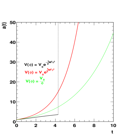
Figure 13: Numerical solutions of equation (19) for the three different field potentials (left). The dotted line in the figure indicates the infinite value. The time variations of the equation state parameter $w$ for all three potentials (right). These plots are obtained by taking constants $k=8\pi G$, $V_{0}$, $M$, $n$ as unity and the initial field value $\phi_{0}$ = 0.1.

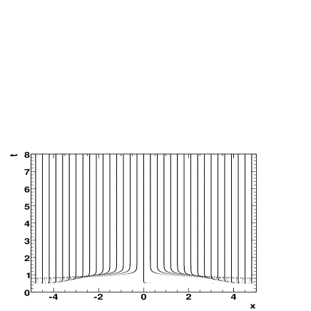
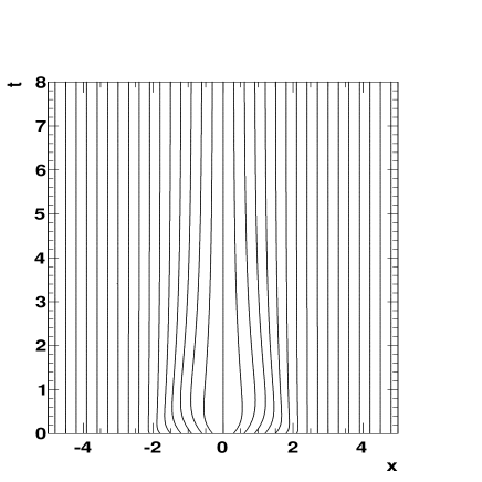
Figure 14: The particle trajectories in FRW expanding universe obtain from equation (23) assuming all time dark energy effect, i. e. with the scale factor $a\sim t^{2/3(1+w)}$ for $w$ = - 0.9 (left) and using the numerical data of solutions of equations (18) and (19) (right) for the inverse power-law field potential (35) and the profile $\phi_{i}(q)=exp(-q^{2})$. Other assumptions for the right panel of this this figure are same as the right panel of the figure 9. We put both left and right panels in this figure to focus on the late time evolution of the field as well as to show that at late times the inverse power-law potentials have exactly same effect on the scalar field as the dark energy has on it.

In view of the aforesaid, we consider the models based upon the inverse power-law potentials more viable than the one with rolling massive scalar field to explain the present accelerated expansion of our universe.

IV Conclusion

In this paper, we have examined the phenomenon of caustic formation in tachyon system with two generic classes of potentials. We presented analytical estimates supported by detailed numerical simulation. We show that the time variation of the scalar field with exponentially decreasing potential, $V=V_{0}e^{-\frac{1}{2}M^{2}\phi^{2}}$, becomes gradually important as the time elapses for both the homogeneous and the inhomogeneous field configurations. There are multi-valued regions and regions of likely to be caustic for this potential in Minkowski space time as well as in FRW expanding universe which broadly agrees with the analysis of Ref. staro . However in the case of the expanding universe, the caustic formations is more definite than the case of 1 + 1 dimensional Minkowski space. It is clearly seen from figure 4 that expansion works against caustic formation: it dilutes the effect of caustics but can not render the situation caustic free in the present case which is generally true for a tachyon potential that decays faster than $1/\phi^{2}$ at infinity.

The field exhibits oscillatory behavior for exponentially increasing rolling massive scalar field potential, $V=V_{0}e^{\frac{1}{2}M^{2}\phi^{2}}$. In the case of inhomogeneous field, the magnitude of time oscillations of the field is very small and hence the field can be considered as almost steady for a sufficiently tuned values of initial parameters. The field with exponentially increasing rolling massive potential is free from caustic formation in both cases of 1 + 1 dimensional Minkowski space and expanding universe, see Fig. 9. It is interesting to note that this potential can give rise to late time acceleration provided that we fine tune the energy scale $V_{0}$ in the potential appropriately.

For inverse power-law potentials, $V(\phi)=V_{0}/\phi^{n},~{}0<n<2$, dark energy is a late time attractor of dynamics and in this case, we did expect the system to be free from caustics. Our analysis shows that the time variation of the homogeneous and inhomogeneous fields are almost similar in this case, because the space variation of the field is insignificant in comparison to time variation. Fig. 12 shows that caustics are formed with the multi-valued regions beyond them in the field configuration in case of inverse power-law potentials in Minkowski space time.

Heuristically speaking, expansion generally works against caustic formation and its effects becomes crucial for inverse power-law potentials with $~{}0<n<2$. If the potential vanishes faster than $1/\phi^{2}$ at infinity, the dust like solution is late time attractor; the exponentially decreasing potential belongs to this category. In this case, caustics form in Minkovski space very distinctly. The cosmic expansion does dilute the effect of caustic formation but can not irradicate them. It is really interesting that for the inverse power law potentials under consideration, the effect of expansion can compete with the tendency of caustic formation. Indeed, dark energy as a late time attractor of the dynamics in this case, gives rise to cosmic repulsion allowing to avoid caustics and multi-valued regions in the field profile.

From the behavior of the scalar field with exponentially increasing and inverse power-law potentials, we infer that field first rolls fast and mimics dark matter and subsequently gives rise to dark energy, see figure 13. Our simulation shows that the particle trajectories computed in the expanding universe using the exact evolution equations (18) and (19) broadly agree with result obtained assuming dark energy dominance at all times.

Evolution of field configurations at different times is similar for the cases of exponentially decreasing rolling massive and inverse power-law potentials apart from the initial and transition periods in the Minkowski space and the expanding universe. It should be noted that in the case of the expanding universe, the pattern of the evolution of the field remains almost same as its initial profile for the scalar field dominated universe. Since the field is almost steady for the exponentially increasing rolling massive scalar potential, the field configuration is same as its initial profile. Thus taking into account the results of Ref. staro , we conclude that caustics generally form for DBI systems in Minkowski space time with an exception of massive rolling scalar. On the other hand in FRW expanding universe, caustics form in DBI systems with potentials decaying faster than $1/\phi^{2}$ at infinity, in particular the exponentially decreasing rolling massive scalar potential. As for the inverse power-law potentials under consideration, they are free from caustics and may be suitable to explain the late time cosmic acceleration.

References

- (1) A. G. Riess et al., Astron. J. 116, 1009 (1998); S. Perlmutter et al., Astrophys. J. 517, 565 (1999); N. A. Bahcall, J. P. Ostriker, S. Perlmutter and P. J. Steinhardt, Science 284, 1481 (1999).
- (2) V. Sahni and A. A. Starobinsky, Int. J. Mod. Phys. D 9, 373 (2000); S. M. Carroll, arXiv:astro-ph/0004075; T. Padmanabhan, Phys. Rept. 380, 235(2003); P. J. E. Peebles and B. Ratra, Rev. Mod. Phys. 75, 559 (2003); E. V. Linder, arXiv:astro-ph/0511197; 1753(2006)[hep-th/0603057]; L. Perivolaropoulos, astro-ph/0601014; N. Straumann, arXiv:gr-qc/0311083.
- (3) E. J. Copeland, M. Sami and S. Tsujikawa, Int. J. Mod. Phys., D15 , 1753(2006)[hep-th/0603057].
- (4) E. V. Linder, astro-ph/0704.2064; J. Frieman, M. Turner and D. Huterer, arXiv:0803.0982; Robert R. Caldwell and Marc Kamionkowski,arXiv:0903.0866; A. Silvestri and Mark Trodden, arXiv:0904.0024.
- (5) I. Zlatev, L. M. Wang and P. J. Steinhardt, Phys. Rev. Lett. 82, 896 (1999); P. J. Steinhardt, L. M. Wang and I. Zlatev, Phys. Rev. D 59, 123504 (1999); L. Amendola, Phys. Rev. D 62, 043511 (2000).
- (6) C. Armendariz-Picon, V. Mukhanov and P. J. Steinhardt, Phys. Rev. Lett. 85, 4438 (2000); Phys. Rev. D 63, 103510 (2001); T. Chiba, T. Okabe and M. Yamaguchi, Phys. Rev. D 62, 023511 (2000).
- (7) A. Y. Kamenshchik, U. Moschella and V. Pasquier, Phys. Lett. B 511, 265 (2001); N. Bilic, G. B. Tupper and R. D. Viollier, Phys. Lett. B 35, 17 (2002); M. C. Bento, O. Bertolami and A. A. Sen, Phys. Rev. D 66, 043507 (2002).
- (8) T. Padmanabhan, Phys. Rev. D 66, 021301 (2002); J. S. Bagla, H. K. Jassal and T. Padmanabhan, Phys. Rev. D 67, 063504 (2003).
- (9) M. R. Garousi, M. Sami and S. Tsujikawa, Phys. Rev. D 70, 043536 (2004); M. R. Garousi, M. Sami and S. Tsujikawa, Phys.Lett. B 606, 1 (2005).
- (10) A. Sen, JHEP 9910, 008 (1999); JHEP 0204, 48 (2002); JHEP 0207, 065 (2002); M. R. Garousi, Nucl. Phys. B 584, 284 (2000); Nucl. Phys. B 647, 117 (2002); JHEP 0304, 027 (2003); JHEP 0305, 058 (2003); JHEP 0312, 036 (2003); E. A. Bergshoeff, M. de Roo, T. C. de Wit, E. Eyras, S. Panda, JHEP 0005, 009 (2000); J. Kluson, Phys. Rev. D 62, 126003 (2000); D. Kutasov and V. Niarchos, Nucl. Phys. B 666, 56 (2003).
- (11) E. J. Copeland, M. R. Garousi, M. Sami , S. Tsujikawa, Phys. Rev. D71, 043003 (2005)[hep-th/0411192].
- (12) S. Tsujikawa and M. Sami, Phys. Lett. B603, 113(2004)[hep-th/0409212]; M. Sami, N. Savchenko and A. Toporensky, Phys. Rev. D70, 123528(2004)[hep-th/0408140].
- (13) L. P. Chimento, Monica Forte, G. M. Kremer and M. O. Ribas, 0809.1919 [gr-qc]; W. Chakraborty, Ujjal Debnath, e-Print: arXiv:0804.4801; I.Ya. Aref’eva and A.S. Koshelev, JHEP 0809:068,2008[0804.3570]; Zong-Kuan Guo and Nobuyoshi Ohta, JCAP 0804:035,2008; M.R. Setare, Phys. Lett. B653, 116(2007); Z. Keresztes, L.A. Gergely, V. Gorini, U. Moschella, A.Yu. Kamenshchik, arXiv:0901.2292.
- (14) T. Padmanabhan, Phys. Rev. D 66, 021301 (2002).
- (15) G. N. Felder, Lev Kofman and A. Starobinsky,JHEP 0209,026(2002)[hep-th/0208019]
- (16) J. S. Bagla, H. K. Jassal and T. Padmanabhan, Phys. Rev. D 67, 063504 (2003).
- (17) L. R. W. Abramo and F. Finelli, Phys. Lett. B 575 (2003) 165.
- (18) J. M. Aguirregabiria and R. Lazkoz, Phys. Rev. D 69, 123502 (2004).
- (19) Z. K. Guo and Y. Z. Zhang, JCAP 0408, 010 (2004).
- (20) M. R. Garousi, M. Sami and S. Tsujikawa, arXiv:hep-th/0412002v1.
- (21) L. R. Abramo and F. Finelli, Phys. Lett. B 575, 165 (2003).
- (22) E. J. Copeland, M. R. Garousi, M. Sami and S. Tsujikawa, arXiv:hep-th/0411192.
- (23) A. Frolov, L. Kofman and A. Starobinsky, Phys Lett. B 545, 8 (2002) [hep-th/0204187v1].
- (24) K. Trenčevski, Gen. Relativ. Gravit. 37(3), 507 (2005).
- (25) J. Lee and S. F. Shandarin, Astrophys. J. 505,L75 (1998).