Equivalence of volume and temperature fluctuations in power-law ensembles

Abstract

Relativistic particle production often requires the use of Tsallis statistics to account for the apparently power-like behavior of transverse momenta observed in the data even at a few GeV/c. In such an approach this behavior is attributed to some specific intrinsic fluctuations of the temperature $T$ in the hadronizing system and is fully accounted by the nonextensivity parameter $q$. On the other hand, it was recently shown that similar power-law spectra can also be obtained by introducing some specific volume fluctuations, apparently without invoking the introduction of Tsallis statistics. We demonstrate that, in fact, when the total energy is kept constant, these volume fluctuations are equivalent to temperature fluctuations and can be derived from them. In addition, we show that fluctuations leading to multiparticle power-law Tsallis distributions introduce specific correlations between the considered particles. We then propose a possible way to distinguish the fluctuations in each event from those occurring from event-to-event. This could have applications in the analysis of high density events at LHC (and especially in ALICE).

1 Introduction

Statistical modelling represents a widely used standard tool to analyze multiparticle production processes [1]. However, this approach does not account for the possible intrinsic nonstatistical fluctuations in the hadronizing system. These usually result in a characteristic power-like behavior of the single particle spectra and in the broadening of the corresponding multiplicity distributions. Such fluctuations are important as they can signal a possible phase transition(s) taking place in an hadronizing system [2], so to include such features, one should base this modelling on the Tsallis statistics [3, 4, 5], leading to a Tsallis distribution, $h_{q}(E)$, which accounts for such situations by introducing in addition to the temperature $T$ a new parameter, $q>1$. This parameter is, as shown in [6, 7], directly connected to fluctuations of the temperature. For $q\rightarrow 1$ one recovers the usual Boltzmann-Gibbs distribution, $f(E)$:

$$h_{q}(E) = \exp_{q}\left(-\frac{E}{T}\right)=\frac{2-q}{T}\left[1-(1-q)\frac{E}{T}\right]^{\frac{1}{1-q}}$$ (1)

$$\stackrel{{\scriptstyle q\rightarrow 1}}{{\Longrightarrow}} f(E)=\frac{1}{T}\exp\left(-\frac{E}{T}\right),$$ (3)

$$q-1=\frac{Var(1/T)}{\langle 1/T\rangle^{2}}.$$

The most recent applications of this approach come from the PHENIX Collaboration at RHIC [8] and from CMS Collaboration at LHC [9] (see also a recent compilation [10]). One must admit at this point, that this approach is subjected to a rather hot debate of whether it is consistent with equilibrium thermodynamics or else it is only a handy way to a phenomenological description of some intrinsic fluctuations in the system [11]. However, as was recently demonstrated on general grounds in [12], fluctuation phenomena can be incorporated into a traditional presentation of thermodynamic and the Tsallis distribution (3) belongs to the class of general admissible distributions which satisfy thermodynamic consistency conditions. They are therefore a natural extension of the usual Boltzman-Gibbs canonical distribution (3).

In fact, as was shown in [6], assuming some simple diffusion picture as responsible for temperature equalization in a nonhomogeneous heat bath (in which local temperature, $T$, fluctuates from point to point around some equilibrium value, $T_{0}$) one gets the evolution of $T$ in the form of a Langevin stochastic equation and distribution of $1/T$, $g(1/T)$, as a solution of the corresponding Fokker-Planck equation. It turns out that $g(1/T)$ has the form of a gamma distribution,

$$g(1/T)=\frac{1}{\Gamma\left(\frac{1}{q-1}\right)}\frac{T_{0}}{q-1}\left(\frac{1}{q-1}\frac{T_{0}}{T}\right)^{\frac{2-q}{q-1}}\cdot\exp\left(-\frac{1}{q-1}\frac{T_{0}}{T}\right).$$ (4)

Convoluting $\exp(-E/T)$ with such $g(1/T)$ one immediately gets Tsallis distribution (1) with a well physically defined parameter $q$: according to Eq. (3) it is entirely given by the temperature fluctuation pattern, which in turn is fully described by the parameters entering this basic diffusion process (like, for example, conductance and specific heat of the hadronic matter consisting this nonhomogeneous heat bath, cf., [6] for details). This approach was recently generalized to account for the possibility of transferring energy from/to a heat bath with a new parameter characterizing the corresponding viscosity entering into the definition of $q$ (it appears to be important for AA applications [4, 16] and for cosmic ray physics [17]; we shall not discuss this issue here) .

In the next Section, we shall discuss the correspondence between fluctuations of volume $V$ proposed in [20] and the presented above fluctuations of temperature $T$ (both result in power-like distributions). Section 3 is devoted to a discussion of some specific $q$-induced correlations and fluctuations. Section 4 is a summary.

2 Fluctuations of $V$ or $T$?

We start by stressing that the form of $g(1/T)$ as given by Eq. (4) is not assumed, but derived from the properties of the underlying physical process in the nonhomogeneous heat bath. Apparently, the same results in what concerns the power-like character of single particle spectra and the broadening of the corresponding multiplicity distributions, $P(N)$, were obtained in [20] without resorting to Tsallis statistics. It was assumed there that the volume $V$ fluctuates in scale invariant way following the KNO form of $P(N)$ deduced from the experiment [21]. We shall now demonstrate that, for the case of constant energy $E$ considered in [20], both approaches are equivalent in the sense that one can start from fluctuations of $V$ and recover fluctuations of $T$ as discussed above, or else, one can start from fluctuations of $T$ as given by $g(1/T)$ and recover fluctuations of $V$ as assumed in [20].

Following the approach of [20], for constant total energy, $E=const$, when both the volume $V$ and temperature $T$ are related via $E\sim VT^{4}$, i.e., when

$$T=\langle T\rangle\left(\frac{\langle V\rangle}{V}\right)^{\frac{1}{4}},$$ (5)

the mean multiplicity in the microcanonical ensemble (MCE), $\bar{N}$, can be written as

$$\bar{N}=\langle N\rangle\cdot\frac{V}{\langle V\rangle}\left(\frac{T}{\langle T\rangle}\right)^{3}=\langle N\rangle\ y\quad{\rm where}\quad y=\left(\frac{V}{\langle V\rangle}\right)^{1/4}.$$ (6)

This relation points to the KNO scaling form of the multiplicity distribution as good candidate for distribution of $y$, which was therefore assumed to be given by [21]

$$\psi(y)=\frac{k^{k}}{\Gamma(k)}y^{k-1}\exp(-ky).$$ (7)

From Eqs. (6) and (5) one gets that

$$y=\frac{\langle T\rangle}{T}.$$ (8)

This means that $T$ fluctuates as well according to the distribution $\psi(\langle T\rangle/T)$. The power-like form of the single particle spectra then follows immediately, all apparently without invoking any reference to Tsallis statistics. This completes the proposed picture which now comprises both fluctuations presented in the multiplicity distribution $P(N)$ (from the scaling form of which one deduces the shape of volume fluctuations) and the power-like behavior of single particle spectra emerging because of temperature fluctuations that follow. Notice now that that $\psi(\langle T\rangle/T)$ assumed here is, in fact, the same distribution as $g(1/T)$ derived in Eq. (4) (with $k=1/(q-1)$, see also Eq. (13) below). So we obtain from $V$ fluctuations the $T$ fluctuations with the same functional form but now without the physical background behind Eq. (4) mentioned above.

However, we can proceed in reverse order and obtain from $T$ fluctuations (4) introduced in Section 1 the fluctuations of $V$ introduced in [20], including the broadening of the corresponding $P(N)$ which takes the form of a NB distribution. This point has been already shown in [24] and we shall quote here its main points for the sake of completeness.

As was proved there, $T$ fluctuations in the form of Eq. (4), discussed in Section 1, result in a specific broadening of the corresponding multiplicity distributions, $P(N)$, which evolve from the poissonian form characteristic for exponential distributions to the negative binomial (NB) form observed for Tsallis distributions. One starts from the known fact that whenever we have $N$ independently produced secondaries with energies $\{E_{i=1,\dots,N}\}$ taken from the exponential distribution $f(E)$, cf. Eq. (3), i.e., when the corresponding joint distribution is given by

$$f\left(\{E_{i=1,\dots,N}\}\right)=\frac{1}{\lambda^{N}}\exp\left(-\frac{1}{\lambda}\sum^{N}_{i=1}E_{i}\right),$$ (9)

and whenever

$$\sum^{N}_{i=0}E_{i}\leq E\leq\sum^{N+1}_{i=0}E_{i},$$ (10)

the corresponding multiplicity distribution is poissonian,

$$P(N)=\frac{\left(\bar{N}\right)^{N}}{N!}\exp\left(-\bar{N}\right)\quad{\rm where}\quad\bar{N}=\frac{E}{\lambda}.$$ (11)

On the other hand, whenever in some process $N$ particles with energies $\{E_{i=1,\dots,N}\}$ are distributed according to the joint $N$-particle Tsallis distribution,

$$h\left(\{E_{i=1,\dots,N}\}\right)\!=\!C_{N}\left[1-(1-q)\frac{\sum^{N}_{i=1}E_{i}}{\lambda}\right]^{\frac{1}{1-q}+1-N}$$ (12)

(for which the corresponding one particle Tsallis distribution function in Eq. (1) is marginal distribution), then, under the same condition (10), the corresponding multiplicity distribution is the NB distribution,

$$P(N)\,=\,\frac{\Gamma(N+k)}{\Gamma(N+1)\Gamma(k)}\frac{\left(\frac{\langle N\rangle}{k}\right)^{N}}{\left(1+\frac{\langle N\rangle}{k}\right)^{(N+k)}};\quad{\rm where}\quad k=\frac{1}{q-1}.$$ (13)

Notice that, in the limiting case of $q\rightarrow 1$, one has $k\rightarrow\infty$ and (13) becomes a poissonian distribution (11), whereas for $q\rightarrow 2$ on has $k\rightarrow 1$ and (13) becomes a geometrical distribution. It is easy to show that for large values of $N$ and $\langle N\rangle$ one obtains from Eq. (13) its scaling form,

$$\langle N\rangle P(N)\cong\psi\left(z=\frac{N}{\langle N\rangle}\right)=\frac{k^{k}}{\Gamma(k)}z^{k-1}\exp(-kz),$$ (14)

in which one recognizes a particular expression of Koba-Nielsen-Olesen (KNO) scaling [21] assumed in [20] to also describe the volume fluctuations, cf. Eq. (7). This result closes the demonstration that, under the condition of constancy of total energy used here, $T$ and $V$ fluctuations are equivalent .

We close this Section with the following remarks. As was said above, $T$ fluctuations are derived from the more realistic description of the nonhomogeneous heat bath, and therefore parameter $q$ and the Tsallis distribution, Eq. (1), reflect the physics of this heat bath. However, one can argue that, on this deeper level, this physics is nothing more than some phenomenological modelling, assumptions of which are reflected in $q$. The $V$ fluctuations approach uses instead as its input the experimental knowledge of the scaling properties of particle multiplicity distributions, $P(N)$, assuming that fluctuations presented there are transmitted to fluctuations of the volume. In fact, fluctuations of $V$ could have some deeper phenomenological foundation, not mentioned in [20]. Namely, it is known that one observes experimentally a variation of the emitting radius (evaluated from the Bose-Einstein correlation analysis) with the charged multiplicity of the event, see, for example, [26]. An increase of about $10$ % of the radius when the multiplicity increases from $10$ to $40$ charged hadrons in the final state was reported. Unfortunately, the quality of data does not allow us to precisely determine the power index of the volume dependence. It is also remarkable that both the energy density, $\rho_{E}=E/V$, and particle density, $\rho_{N}=N/V$, decrease for large multiplicity events. For $N/\langle N\rangle\sim y$ one observes $\rho_{E}/\langle\rho_{E}\rangle\sim y^{-4}$ and $\rho_{N}/\langle\rho_{N}\rangle\sim y^{-3}$. All these features deserve further consideration and should be checked in LHC experiments, especially in ALICE, which is dedicated to heavy ion collision.

3 Some consequences of $q$ statistics

We would like to close with a short discussion of some consequences of $q$-statistics which can a priori be subjected to experimental verification: the $q$-induced correlations and event-by-event fluctuations.

The $q$-induced correlations occur in a natural way in an $N$-particle Tsallis distribution introduced in Eq. (12). For Boltzmann-Gibbs statistics, for $N$ independently produced particles, the joint distribution (9) can be written in factorizable form as a simple product of single particle distributions,

$$f\left(\{E_{i=1,\dots,N}\}\right)=\prod_{i=1}^{N}f\left(E_{i}\right).$$ (15)

However, such a product of single particle Tsallis distributions does not result in an $N$-particle Tsallis distribution [24]. To get Eq. (12) one has to fluctuate the temperature in the distribution $f\left(\{E_{i=1,\dots,N}\}\right)$ above, i.e.,

$$h\left(\{E_{i=1,\dots,N}\}\right)\!\!=\!\!\int^{\infty}_{0}\!\!\!f\left(\{E_{i=1,\dots,N}\}\right)g(1/T)d(1/T).$$ (16)

This procedure introduces correlations between particles. The corresponding covariance, $Cov\left(E_{i},E_{j}\right)$, and correlation coefficient, $\rho$, for energies are equal to

$$Cov\left(E_{i},E_{j}\right)=\frac{\lambda^{2}(q-1)}{(3-2q)^{2}(4-3q)},$$ (17)

$$\rho=\frac{1}{2-q}-1.$$ (18)

As an illustrative example, we calculate the two-particle correlation function

$$C_{2}\left(E_{i},E_{j}\right)=\frac{h\left(E_{i},E_{j}\right)}{h\left(E_{i}\right)h\left(E_{j}\right)}.$$ (19)

This is shown in Fig. 1 for different values of variables $\delta$ and $\sigma$,

$$\delta=\frac{E_{i}-E_{j}}{T}\quad{\rm and}\quad\sigma=\frac{E_{i}+E_{j}}{T}.$$ (20)

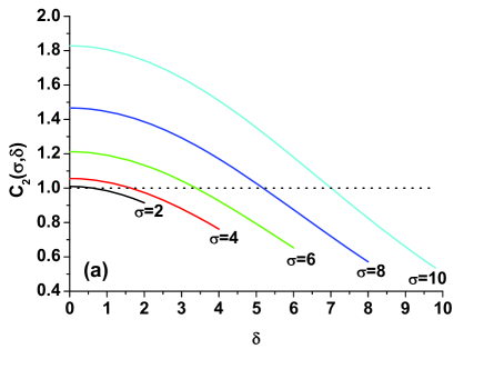
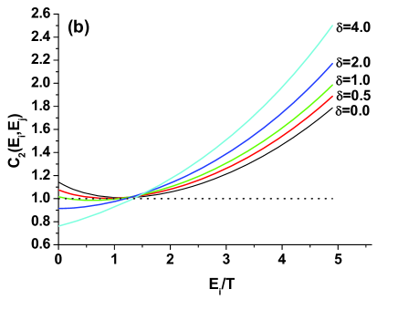
Figure 1: (Color online). Two-particle correlation function $C_{2}\left(E_{i},E_{j}\right)$ for Tsallis distribution with the parameter $q=1.125$.

Notwithstanding the rather complicated dependencies shown in Fig. 1, the distance distribution, $h_{q}$ defined as

$$h_{q}(\delta)=\int^{\infty}_{0}h_{q}\left(E_{i},E_{i}+\delta\right)dE_{i}$$ (21)

for variables sampled from the joint distribution (12) is given by a Tsallis distribution

$$h_{q}(\delta)=\frac{2-q}{2}[1-(1-q)\delta]^{\frac{1}{1-q}}$$ (22)

(analogously as the distance distribution for the exponentially distributed variables is given by exponential distribution, to which (21) converges for $q\rightarrow 1$).

In what concerns event-by-event fluctuations there are two types of fluctuations one can encounter, namely fluctuations from event to event or fluctuations in each event. Two scenarios are possible here.

• In the first, $T$ (and/or $V$) are constant in each event. However, because of different initial conditions, they fluctuate from event to event. In this case, in each event one should find an exponential dependence (3) with $T=T_{k}$ and a possible departure from it could occur only after averaging over all $N_{ev}$ events, $k=1,2,\dots,N_{ev}$. It will reflect fluctuations originating in the different initial conditions collision from which a given event originates. Only inclusive distributions will be described by a Tsallis formula (1). Such a situation was discussed above.

• In the other scenario, $T$ fluctuates in each event around some value $T_{0}$. In this case one should observe a departure from the exponential behavior already on the single event level and it should follow Eq. (1) with $q>1$. This reflects the situation when, due to some intrinsically dynamical reasons, different parts of a given event can have different temperatures [6, 4]. For volume fluctuations such a scenario seems to be unrealistic.

In [27] we argued that event-by-event analysis of multiparticle production data are an ideal place to search for a possible fluctuation of the temperature characterizing a hadronizing source using the thermodynamical approach. Namely, an analysis of the transverse momentum spectra in $Pb+Pb$ collisions at TeV energies of LHC (mainly in ALICE experiment) should allow us to distinguish between both scenarios listed above. The LHC is designed for colliding proton-proton and nucleus-nucleus beams up to $\sqrt{s}=14$ TeV [28]. Collisions at these unprecedented high energies will provide opportunities for new types of analysis. In proton-proton collisions at the highest possible energy, the expected charged particle multiplicity is only $\sim 10$ at the midrapidity region ( $|\eta|<0.5$) and it is roughly five times bigger in the full rapidity region [29] (the ALICE experiment has the possibility of measuring the distributions over the $-5.0<\eta<3.5$ range, but the CMS and ATLAS experiments have a more limited coverage of $|\eta|<2.5$ units). The most important fact is that, in heavy ion collisions we have $\sim A$ higher multiplicities (for central $Pb+Pb$ collisions one expects $\sim 2500$ particles at allowed rapidity acceptance region). This is enough to analyze event-by-event distributions over $3$ orders of magnitude, which should allow us to determine the shape of the distribution in a single event. Moreover, in such circumstances we should be able to also construct the distribution $dN/d\delta$ for $\delta=p_{Ti}-p_{Tj}$ for $N(N-1)\cong 6\cdot 10^{6}$ pairs in an event, over $6$ orders of magnitude and using Eq. (21) test the above possible scenarios. Eq. (21) tells us that, instead of distributions of $p_{T}$, $dN/dp_{T}$, one can use distributions $dN/d\delta$ and look whether it follows the Tsallis form on an event-by-event basis. Because for Eq. (21) one has $N(N-1)$ entries to be compared with only $N$ for $p_{T}$ distributions, one expects that the distribution Eq. (21) will reach further and it would be easier to differentiate between the Tsallis distribution and the usual exponential one.

Figure 2: (Color online). The sensitivity to the parameter $q$ of $(a)$ the correlation function $C_{2}(\sigma,\delta)$ with $\sigma=6$ and $(b)$ the distribution of $\delta$, $h(\delta)$, with error band corresponding to the event multiplicity $N=10^{3}$.

Fig. 2a presents the sensitivity of the correlation function $C_{2}(\sigma,\delta)$ to different values of the parameter $q$ chosen. Similarly, Fig. 2b presents sensitivity of the proposed method in the event-by-event analysis on the example of distribution $h(\delta)$ plotted for different values of the parameter $q$ with error bands corresponding to the event with multiplicity $N=10^{3}$.

We close this Section with a few remarks on what can be deduced from existing experimental data. To separate the two scenarios presented here one could, for example, use the analysis of event-by-event fluctuations of the average transverse momenta $\bar{p_{T}}$ presented at RHIC experiments. STAR data [30] show that $Var\left(\bar{p_{T}}\right)/\langle\bar{p_{T}}\rangle^{2}\cong 10^{-4}$, where $\bar{p_{T}}$ denotes averaging in an event and $\langle\bar{p_{T}}\rangle$ is the overall event average. In the above estimation $Var\left(\bar{p_{T}}\right)=Var\left(\bar{p_{T}}\right)_{data}-Var\left(\bar{p_{T}}\right)_{mixed}$. STAR [30] measured also the quantity $\langle\Delta p_{Ti}\Delta p_{Tj}\rangle=Cov\left(p_{Ti},p_{Tj}\right)-Var\left(\bar{p_{T}}\right)$. In this case $\Delta p_{Ti}=p_{Ti}-\langle\bar{p_{T}}\rangle$ was estimated without using mixed event and the resulting value of fluctuations was the same as above (cf. also [24]). Therefore, in the scenario of volume fluctuations (or temperature fluctuations occurring from event to event), assuming that $\bar{p_{T}}\propto T$, we obtain $Var(T)/\langle T\rangle^{2}=Var\left(\bar{p_{T}}\right)/\langle\bar{p_{T}}\rangle^{2}\cong 10^{-4}$, leading to $q-1\cong 10^{-4}$. This is much smaller than the value $q-1\cong 10^{-2}$ estimated from transverse momenta distributions [4, 8, 9]. However, if the temperature $T$ fluctuates within the event (for example, is different in every inter-nuclear collisions), we expect that for the $N_{P}$ projectile participants $Var\left(\bar{p_{T}}\right)\cong Var(T)/N_{P}$. In this case, for $N_{P}\cong 100$ the relative fluctuations are $Var(T)/\langle T\rangle^{2}\cong 10^{-2}$, i.e., are comparable to those obtained from the transverse momentum distributions mentioned above. Similar estimations could be made also for [31] data. A more detailed analysis of this type is outside the scope of this paper and will be presented elsewhere.

4 Summary

To summarize: we have demonstrated that two approaches to fluctuation phenomena observed in multiparticle production processes as power law distributions or broadening of the corresponding multiplicity distributions, the one based on temperature fluctuations [6, 24] and the one based on volume fluctuations [20] can be regarded, as long as the corresponding total energy is kept constant, to be equivalent. One can be deduced from the other. We have also shown that fluctuations which lead to multiparticle power-law distributions introduce some specific correlations between particles in the ensemble of particles considered and propose a way to distinguish the fluctuations in each event from those occurring from event-to-event by analyzing the distance distribution, Eq. (21). On the other hand, it seems that the already existing RHIC data on $p_{T}$ correlations [30, 31] can also be useful to obtain such information (this point demands, however, a more detailed study).

References

References

- [1] See, for example, Gaździcki M, Gorenstein M, and P. Seybothe, Acta Phys. Polon. B 42 (2011) 307 and references therein.
- [2] Stodolsky L 1995 Phys. Rev. Lett. 75 1044; Heiselberg H 2001 Phys. Rep. 351 161; Mrówczyński S 2009 Acta Phys. Pol. B 40 1053
- [3] Tsallis C, J. 1988 Stat. Phys. 52 479; Salinas S R A, and Tsallis C (eds.), 1999 Special Issue on Nonextensive Statistical Mechanics and Thermodynamic, Braz. J. Phys. 29; Gell-Mann M, and Tsallis C (Eds.) 2004 Nonextensive Entropy Interdisciplinary Applications (Oxford University Press, New York); Tsallis C 2009 Eur. Phys. J. A 40 257
- [4] Wilk G, and Włodarczyk Z 2009 Eur. Phys. J. A 40 299
- [5] Biró T S, Purcel G, and Ürmösy K 2009 Eur. Phys. J. A 40, 325 (2009)
- [6] Wilk G, and Włodarczyk Z 2000 Phys. Rev. Lett. 84 1770 and 2001 Chaos, Solitons and Fractals 13/3 581
- [7] Biró T S, and Jakovác A 2005 Phys. Rev. Lett. 94 132302
- [8] Adare A et al. (PHENIX Coll.), Measurement of neutral mesons in collisions at GeV and scaling properties of hadron production, arXiv:1005.3674[hep-exp], to be published in Phys. Rev. D
- [9] Khachatryan V et al. (CMS Collaboration) 2010 J. High Energy Phys.02 041
- [10] Ming Shao, Li Yi, Zebo Tang, Hongfang Chen, Cheng Li, and Zhangbu Xu (2010) J. Phys. G 37 085104.
- [11] Nauenberg M 2003 Phys. Rev. E 67 036114 and 2004 Phys. Rev. E 69 038102; Tsallis C 2004 Phys. Rev. E 69 038101; Balian R, and Nauenberg M 2006 Europhysics News 37 9; Luzzi R, Vasconcellos A R, and Galvao Ramos J 2006 Europhysics News 37 11
- [12] Maroney O J E 2009, Phys. Rev E 80 061141
- [13] Biró T S, Ürmösy K, and Schram Z 2010 J. Phys. G 37 094027
- [14] Osada T, and Wilk G 2008 Phys. Rev. C 77 044903
- [15] Rożynek J, and Wilk G 2009 J. Phys. G 36 125108; Alberico W M, and Lavagno A 2009 Eur. Phys. J. A 40 313; Lavagno A, Pigato D, and Quarati P 2010 J. Phys. G 37 115102
- [16] Wilk G, and Włodarczyk Z 2009 Phys. Rev. C 79 054903
- [17] Wilk G, and Włodarczyk Z (2010) Cent. Eur. J. Phys. 8 726
- [18] Gorenstein M I, and Hauer M 2008 Phys. Rev. C 78 041902(R)
- [19] Beck C, and Cohen E G D 2003 Physica A 322 267; Sattin F 2006 Eur. Phys. J. B 49 219
- [20] Begun V V, Gaździcki M, and Gorenstein M I 2008 Phys. Rev. C 7̱8 024904
- [21] Koba Z, Nielsen H B, and Olesen P 1972 Nucl. Phys. B 40 319. For the most recet review of this subject see: Fiete Grosse-Oetringhaus J F, and Reygers K 2010 J. Phys. G 37 083001
- [22] Alner G J et al. (UA5 Collaboration) 1987 Phys. Rep. 154 247
- [23] Geich-Gimbel C 1989 Int. J. Mod. Phys. A 4 1527
- [24] Wilk G, and Włodarczyk Z 2007 Physica A 376 279
- [25] Rybczyński M, Włodarczyk Z, and Wilk G, 2003 Nucl. Phys. B (Proc. Suppl.) 1̱22 325; Navarra F S, Utyuzh O V, Wilk G, and Włodarczyk Z 2003 Phys. Rev. D 67 114002
- [26] Alexander G et al. (OPAL Collaboration) 1996 Z. Phys. C 72 389; Giacomelli G 1991 Nucl. Phys. Proc. Suppl. B 25 30; Breakstone A et al. 1985 Phys. Lett. B 162 400
- [27] Wilk G, and Włodarczyk Z 2002 Physica A 305 227
- [28] See, for example, Alessandro A et al. (ALICE Collaboration) 2006 J. Phys. G 32 1295; d Enterria D G et al. (CMS Collaboration) 2007 J. Phys. G 34 2307; Bayatian G L et al. (CMS Collaboration) 2007 J. Phys. G 34 995; Aad D et al. (ATLAS Collaboration), Expected Performance of the ATLAS Experiment - Detector, Trigger and Physics, arXiv:0901.0512[hep-ex]
- [29] Dash A K, and Mohanty B 2010 J. Phys. G 37 025102
- [30] Adams J et al (STAR Collaboration) 2005 Phys. Rev. C 72 044902
- [31] Adox K et al (PHENIX Collaboration) 2002 Phys. Rev. C 66 024901