Gaussian Mixture Modeling with Gaussian Process Latent Variable Models

Abstract

Density modeling is notoriously difficult for high dimensional data. One approach to the problem is to search for a lower dimensional manifold which captures the main characteristics of the data. Recently, the Gaussian Process Latent Variable Model (GPLVM) has successfully been used to find low dimensional manifolds in a variety of complex data. The GPLVM consists of a set of points in a low dimensional latent space, and a stochastic map to the observed space. We show how it can be interpreted as a density model in the observed space. However, the GPLVM is not trained as a density model and therefore yields bad density estimates. We propose a new training strategy and obtain improved generalisation performance and better density estimates in comparative evaluations on several benchmark data sets.

Modeling of densities, aka unsupervised learning, is one of the central problems in machine learning. Despite its long history [1], density modeling remains a challenging task especially in high dimensional spaces. For example, the generative approach to classification requires density models for each class, and training such models well is generally considered more difficult than the alternative discriminative approach. Classical approaches to density modeling include both parametric and non parametric methods. In general, simple parametric approaches have limited utility, as the assumptions might be too restrictive. Mixture models, typically trained using the EM algorithm, are more flexible, but e.g. Gaussian mixture models are hard to fit in high dimensions, as each component is either diagonal or has in the order of $D^{2}$ parameters, although the mixtures of Factor Analyzers algorithm [2] may be able to strike a good balance. Methods based on kernel density estimation [3, 4] are another approach, where bandwidths may be set using cross validation [5].

The methods mentioned so far have two main shortcomings: 1) they typically do not perform well in high dimensions, and 2) they do not provide an intuitive or generative understanding of the data. Generally, we can only succeed if the data has some regular structure, the model can discover and exploit. One attempt to do this is to assume that the data points in the high dimensional space lie on – or close to – some smooth underlying lower dimensional manifold. Models based on this idea can be divided into models based on implicit or explicit representations of the manifold. An implicit representation is used by [6] in a non-parametric Gaussian mixture with adaptive covariance to every data point. Explicit representations are used in the Generative Topographic Map [7] and by [8]. Within the explicit camp, models contain two separate parts, a lower dimensional latent space equipped with a density, and a function which maps points from the low dimensional latent space to the high dimensional space where the observations lie. Advantages of this type of model include the ability to understand the structure of the data in a more intuitive way using the latent representation, as well as the technical advantage that the density in the observed space is automatically properly normalised by construction.

The Gaussian Process Latent Variable Model (GPLVM) [9] uses a Gaussian process (GP) [10] to define a (stochastic) map between a lower dimensional latent space and the observation space. However, the GPLVM does not include a density in the latent space. In this paper, we explore extensions to the GPLVM based on densities in the latent space. One might assume that this can trivially be done, by thinking of the latent points learnt by the GPLVM as representing a mixture of delta functions in the latent space. Since the GP based map is stochastic, it induces a proper mixture in the observed space. However, this formulation is unsatisfactory, because the resulting model is not trained as a density model. Consequently, our experiments show poor density estimation performance.

Mixtures of Gaussians form the basis of the vast majority of density estimation algorithms. Whereas kernel smoothing techniques can be seen as introducing a mixture component for each data point, infinite mixture models [11] explore the limit as the number of components increases and mixtures of factor analysers impose constraints on the covariance of individual components. The algorithm presented in this paper can be understood as a method for stitching together Gaussian mixture components in a way reminiscent of [8] using the GPLVM map from the lower dimensional manifold to induce factor analysis like constraints in the observation space. In a nutshell, we propose a density model in high dimensions by transforming a set of low-dimensional Gaussians with a GP.

We begin by a short introduction to the GPLVM and show how it can be used to define density models. In section 2, we introduce a principled learning algorithm, and experimentally evaluate our approach in section 3.

1 The GPLVM as a Density Model

A GP $f$ is a probabilistic map parametrised by a covariance $k(\mathbf{x},\mathbf{x}^{\prime})$ and a mean $m(\mathbf{x})$. We use $m(\mathbf{x})\equiv 0$ and automatic relevance determination (ARD) $k(\mathbf{x}^{i},\mathbf{x}^{j})=\sigma_{f}^{2}\exp\big{(}\!-\frac{1}{2}(\mathbf{x}^{i}-\mathbf{x}^{j})^{\top}\mathbf{W}^{-1}(\mathbf{x}^{i}-\mathbf{x}^{j})\big{)}+\delta_{ij}\sigma_{\eta}^{2}$ in the following. Here, $\sigma_{f}^{2}$ and $\sigma_{\eta}^{2}$ denote the signal and noise variance, respectively and the diagonal matrix $\mathbf{W}$ contains the squared length scales. Since a GP is a distribution over functions $f:\mathcal{X}\rightarrow\mathcal{Z}$, the output $\mathbf{z}=f(\mathbf{x})$ is random even though the input $\mathbf{x}$ is deterministic. In GP regression, a GP prior is combined with training data $\{\mathbf{x}^{i},z^{i}\}_{i\in\mathcal{I}=\{1..N\}}$ into a GP posterior conditioned on the training data with mean $\mu_{*}(\mathbf{x}_{*})=\bm{\alpha}^{\top}\mathbf{k}_{*}$ and covariance $\bar{k}(\mathbf{x}_{*},\mathbf{x}^{\prime}_{*})=k(\mathbf{x}_{*},\mathbf{x}^{\prime}_{*})-\mathbf{k}_{*}^{\top}\mathbf{K}^{-1}\mathbf{k}^{\prime}_{*}$ where $\mathbf{k}_{*}=[k(\mathbf{x}^{1},\mathbf{x}_{*}),..,k(\mathbf{x}^{N},\mathbf{x}_{*})]^{\top}$, $\mathbf{K}=[k(\mathbf{x}^{i},\mathbf{x}^{j})]_{ij=1..N}$, $\bm{\Sigma}_{*}=[\bar{k}(\mathbf{x}^{i},\mathbf{x}^{j})]_{ij=1..N}$ and $\bm{\alpha}^{\top}=[z^{1},..,z^{N}]\mathbf{K}^{-1}$. Deterministic inputs $\mathbf{x}$ lead to Gaussian outputs and Gaussian inputs lead to non-Gaussian outputs whose first two moments can be computed analytically [12] for ARD covariance. Multivariate deterministic inputs $\mathbf{x}$ lead to spherical Gaussian outputs $\mathbf{z}$ and Gaussian inputs $\mathbf{x}$ lead to non-Gaussian outputs $\mathbf{z}$ whose moments $(\bm{\mu}_{*},\bm{\Sigma}_{*})$ are given by:

$\mathbf{x}\sim\delta(\mathbf{x}_{*})\stackrel{{\scriptstyle f\sim\mathcal{GP}}}{{\longrightarrow}}\mathbf{z}\sim\mathcal{N}(\bm{\mu}_{*},\sigma_{*}^{2}\mathbf{I})$		$\mathbf{x}\sim\mathcal{N}(\mathbf{x}_{*},\mathbf{V}_{\mathbf{x}})\stackrel{{\scriptstyle f\sim\mathcal{GP}}}{{\longrightarrow}}\mathbf{z}\stackrel{{\scriptstyle(\approx)}}{{\sim}}\mathcal{N}(\bm{\mu}_{*},\bm{\Sigma}_{*})$
$\bm{\mu}_{*}=\mathbf{A}^{\top}\tilde{\mathbf{k}}_{*}$	$\sigma_{*}^{2}=k_{**}-\mathbf{k}_{*}^{\top}\mathbf{K}^{-1}\mathbf{k}_{*}\in[\sigma_{\eta}^{2},\sigma_{\eta}^{2}+\sigma_{f}^{2}]$	$\bm{\mu}_{*}=\mathbf{A}^{\top}\tilde{\mathbf{k}}_{*}$	$\bm{\Sigma}_{*}=\left(k_{**}-\textrm{tr}(\mathbf{K}^{-1}\hat{\mathbf{K}}_{*})\right)\mathbf{I}+\mathbf{A}^{\top}(\hat{\mathbf{K}}_{*}-\tilde{\mathbf{k}}_{*}\tilde{\mathbf{k}}_{*}^{\top})\mathbf{A}$

Here, $\mathbf{A}^{\top}=[\bm{\alpha}_{1},..,\bm{\alpha}_{D}]^{\top}=[\mathbf{z}^{1},..,\mathbf{z}^{N}]\mathbf{K}^{-1}$ and the quantities $\tilde{\mathbf{k}}_{*}=\mathbb{E}[\mathbf{k}]$ and $\hat{\mathbf{K}}_{*}=\mathbb{E}[\mathbf{k}\mathbf{k}^{\top}]$ denote expectations of $\mathbf{k}=\mathbf{k}(\mathbf{x})=[k(\mathbf{x}^{1},\mathbf{x}),..,k(\mathbf{x}^{N},\mathbf{x})]^{\top}$ w.r.t. the Gaussian input distribution $\mathcal{N}(\mathbf{x}|\mathbf{x}_{*},\mathbf{V}_{\mathbf{x}})$ that can readily be evaluated in closed form [12] as detailed in the Appendix. In the limit of $\mathbf{V}_{\mathbf{x}}\rightarrow\mathbf{0}$ we recover the deterministic case as $\tilde{\mathbf{k}}_{*}\rightarrow\mathbf{k}_{*}$, $\hat{\mathbf{K}}_{*}\rightarrow\mathbf{k}_{*}\mathbf{k}_{*}^{\top}$ and $\bm{\Sigma}_{*}\rightarrow\sigma_{*}^{2}\mathbf{I}$. Non-zero input variance $\mathbf{V}_{\mathbf{x}}$ results in full non-spherical output covariance $\bm{\Sigma}_{*}$, even for independent GPs because all the GPs are driven by the same (uncertain) input.

A GPLVM [9] is a successful and popular non-parametric Bayesian tool for high dimensional nonlinear data modeling taking into account the data’s manifold structure based on a low-dimensional representation. High dimensional data points $\mathbf{z}^{i}\in\mathcal{Z}\subset\mathbb{R}^{D}$, $\mathbf{Z}=[\mathbf{z}^{1},\dots,\mathbf{z}^{N}]$, are represented by corresponding latent points $\mathbf{X}=[\mathbf{x}^{1},\dots,\mathbf{x}^{N}]$ from a low-dimensional latent space $\mathcal{X}\subset\mathbb{R}^{d}$ mapped into $\mathcal{Z}$ by $D$ independent GPs $f_{j}$ – one for each component $z_{j}$ of the data. All the GPs $f_{j}$ are conditioned on $\mathbf{X}$ and share the same covariance and mean functions. The model is trained by maximising the sum of the log marginal likelihoods over the $D$ independent regression problems with respect to the latent points $\mathbf{X}$.

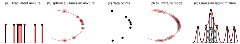
Figure 1: The high dimensional ($D=2$) density of the data points $\mathbf{z}^{i}$ in panel (c) is modelled by a mixture of Gaussians $\mathbb{P}(\mathbf{z})=\frac{1}{N}\sum_{i}\mathcal{N}(\mathbf{z}|\bm{\mu}_{\mathbf{x}^{i}},\bm{\Sigma}_{\mathbf{x}^{i}})$ shown in panel (b,d) where the means $\bm{\mu}_{\mathbf{x}^{i}}$ and variances $\bm{\Sigma}_{\mathbf{x}^{i}}$ are given by the predictive means and covariances of a set of independent Gaussian processes $f_{j}:\mathcal{X}\rightarrow\mathcal{Z}$ conditioned on low-dimensional ($d=1$) latent locations $\mathbf{x}^{i}$. A latent Dirac mixture (a) yields a spherical Gaussian mixture with varying widths (b) and a latent Gaussian mixture (e) results in a fully coupled mixture model (d) smoothly sharing covariances across mixture components.

While most often applied to nonlinear dimensionality reduction, the GPLVM can also be used as a tractable and flexible density model in high dimensional spaces as illustrated in Figure 1. The basic idea is to interpret the latent points $\mathbf{X}$ as centres of a mixture of either Dirac (Figure 1a) or Gaussian (Figure 1e) distributions in the latent space $\mathcal{X}$ that are projected forward by the GP to produce a high dimensional Gaussian mixture $\mathbb{P}(\mathbf{z})=\frac{1}{N}\sum_{i}\mathcal{N}(\mathbf{z}|\bm{\mu}_{\mathbf{x}^{i}},\bm{\Sigma}_{\mathbf{x}^{i}})$ in the observed space $\mathcal{Z}$. Depending on the kind of latent mixture, the density model $\mathbb{P}(\mathbf{z})$ will either be a mixture of spherical (Figure 1b) or full-covariance Gaussians (Figure 1d). By that mechanism, we get a tractable high dimensional density model $\mathbb{P}(\mathbf{z})$: A set of low-dimensional coordinates in conjunction with a probabilistic map $f$ yield a mixture of high dimensional Gaussians whose covariance matrices are smoothly shared between components. As shown in Figure 1(d), the model is able to capture high dimensional covariance structure along the data manifold by relatively few parameters (compared to $D^{2}$), namely the latent coordinates $\mathbf{X}\in\mathbb{R}^{d\times N}$ and the hyperparameters $\bm{\theta}=[\mathbf{W},\sigma_{f},\sigma_{\eta},\mathbf{V}_{\mathbf{x}}]\in\mathbb{R}_{+}^{2d+2}$ of the GP.

The role of the latent coordinates $\mathbf{X}$ is twofold: they both define the GP, mapping the latent points into the observed space, and they serve as centres of the mixture density in the latent space. If the latent density is a mixture of Gaussians, the centres of these Gaussians are used to define the GP map, but the full Gaussians (with covariance $\mathbf{V}_{\mathbf{x}}$) are projected forward by the GP map.

2 Learning Algorithm

Learning or model fitting is done by minimising a loss function $L$ w.r.t. the latent coordinates $\mathbf{X}$ and the hyperparameters $\bm{\theta}$. In the following, we will discuss the usual GPLVM objective function, make clear that it is not suited for density estimation and use leave-out estimation to avoid overfitting.

2.1 GPLVM likelihood

A GPLVM [9] is trained by setting the latent coordinates $\mathbf{X}$ and the hyperparameters $\bm{\theta}$ to maximise the probability of the data

$$\mathbb{P}(\mathbf{Z}|\mathbf{X},\bm{\theta})=\prod_{j=1}^{D}\mathbb{P}(\mathbf{z}_{j}|\mathbf{X},\bm{\theta})=-\frac{DN}{2}\ln 2\pi-\frac{D}{2}\ln\left|\mathbf{K}\right|-\frac{1}{2}\textrm{tr}\left(\mathbf{K}^{-1}\mathbf{Z}^{\top}\mathbf{Z}\right)$$ (1)

that is the product of the marginal likelihoods of $D$ independent regression problems. Using $\frac{\partial L}{\partial\mathbf{K}}\negthickspace=\negthickspace\frac{1}{2}\mathbf{K}^{-1}(\mathbf{Z}^{\top}\mathbf{Z}\negmedspace-\negmedspace D\mathbf{K})\mathbf{K}^{-1}$, conjugate gradients optimisation at a cost of $\mathcal{O}(DN^{3})$ per step is straightforward but suffers from local optima.

However, optimisation of $L_{Z}(\mathbf{X},\bm{\theta})$ does not encourage the GPLVM to be a good density model. Only indirectly, we expect the predictive variance to be small (implying high density) in regions supported by many data points. The main focus of $L_{Z}(\mathbf{X},\bm{\theta})$ is on faithfully predicting $\mathbf{Z}$ from $\mathbf{X}$ (as implemented by the fidelity trace term) while using a relatively smooth function (as favoured by the log determinant term). Therefore, we propose a different cost function.

2.2 General leave-out estimators

Density estimation [13] constructs parametrised estimators $\hat{\mathbb{P}}_{\bm{\theta}}(\mathbf{z})$ from iid data $\mathbf{z}^{i}\sim\mathbb{P}(\mathbf{z})$. We use the Kullback-Leibler divergence $J(\bm{\theta})\stackrel{{\scriptstyle\text{c}}}{{=}}-\int\mathbb{P}(\mathbf{z})\ln\hat{\mathbb{P}}_{\bm{\theta}}(\mathbf{z})\text{d}\mathbf{z}$ to the underlying density and its empirical estimate $\hat{J}_{e}(\bm{\theta})=-\sum_{i\in I}\ln\hat{\mathbb{P}}_{\bm{\theta},I}(\mathbf{z}^{i})$ as quality measure where $I$ emphasises that the full dataset has been used for training. This estimator, is prone to overfitting if used to adjust the parameters via $\bm{\theta}^{*}=\arg\min_{\bm{\theta}}\hat{J}_{e}(\bm{\theta})$. Therefore, estimators based on $K$ subsets of the data $\hat{J}_{v}(\bm{\theta})=-\frac{1}{K}\sum_{k=1}^{K}\sum_{i\notin I_{k}}\ln\hat{\mathbb{P}}_{\bm{\theta},I_{k}}(\mathbf{z}^{i}),\quad I_{k}\subset I$ are used. Two well known instances are $K$-fold cross-validation (CV) and leave-one-out (LOO) estimation. The subsets for CV are $I_{k}\cap I_{k^{\prime}}=\emptyset,I=\bigcup_{k=1}^{K}I_{k},|I_{k}|\approx|I_{k^{\prime}}|$ and $K=N,I_{k}=I\backslash\{k\}$ for LOO. Both of them can be used to optimise $\bm{\theta}$.

2.3 GPLVM leave-one-out density

There are two reasons why training a GPLVM with the log likelihood of the data $L_{Z}(\mathbf{X},\bm{\theta})$ (Eq. 1) is not optimal in the setting of density estimation: Firstly, it treats the task as regression, and doesn’t explicitly worry about how the density is spread in the observation space. Secondly, our empirical results (see Section 3) indicate, that the test set performance is simply not good. Therefore, we propose to train the model using the leave-out density

$$-L_{LOO}(\mathbf{X},\bm{\theta})=\ln\prod_{i=1}^{N}\mathbb{P}_{\neg i}(\mathbf{z}^{i})=\sum_{i=1}^{N}\ln\frac{1}{N-1}\sum_{j\neq i}\mathcal{N}\left(\mathbf{z}^{i}|\bm{\mu}_{\mathbf{x}^{j}},\bm{\Sigma}_{\mathbf{x}^{j}}\right).$$ (2)

This objective is very different from the GPLVM criterion as it measures how well a data point is explained under the mixture models resulting from projecting each of the latent mixture components forward; the leave-out aspect enforces that the point $\mathbf{z}^{i}$ gets assigned a high density even though the mixture component $\mathcal{N}\left(\mathbf{z}^{i}|\bm{\mu}_{\mathbf{x}^{i}},\bm{\Sigma}_{\mathbf{x}^{i}}\right)$ has been removed from the mixture. The leave-one-out idea is trivial to apply in a mixture setting by just removing the contribution in the sum over components, and is motivated by the desire to avoid overfitting. Evaluation of $L_{LOO}(\mathbf{X},\bm{\theta})$ requires $\mathcal{O}(DN^{3})$ assuming $N>D>d$.

However, removing the mixture component is not enough since the latent point $\mathbf{x}^{i}$ is still present in the GP. Using rank one updates to compute inverses and determinants of covariance matrices $\mathbf{K}_{\neg i}$ with row and column $i$ removed, it is possible to evaluate Eq. 3 for mixture components $\mathcal{N}\left(\mathbf{z}^{i}|\bm{\mu}_{\mathbf{x}^{j}}^{\neg i},\bm{\Sigma}_{\mathbf{x}^{j}}\right)$ with latent point $\mathbf{x}^{i}$ removed from the mean prediction $\bm{\mu}_{\mathbf{x}^{j}}^{\neg i}$ – which is what we do in the experiments. Unfortunately, going further by removing $\mathbf{x}^{i}$ also from the covariance $\bm{\Sigma}_{\mathbf{x}^{j}}$ increases the computational burden to $\mathcal{O}(DN^{4})$ because we need to compute rank one corrections to all matrices $\hat{\mathbf{K}}_{\ell},\ \ell=1..N$. Since $\bm{\Sigma}_{\mathbf{x}^{j}}^{\neg i}$ is only slightly smaller than $\bm{\Sigma}_{\mathbf{x}^{j}}$, we refrain from computing it in the experiments.

In the original GPLVM, there is a clear one-to-one relationship between latent points $\mathbf{x}^{i}$ and data points $\mathbf{z}^{i}$ – they are inextricably tied together. However, the leave-one-out (LOO) density $L_{LOO}(\mathbf{X},\bm{\theta})$ does not impose any constraint of that sort. The number of mixture components does not need to be $N$, in fact we can choose any number we like. Only the data visible to the GP $\{\mathbf{x}^{j},\bar{\mathbf{z}}^{j}\}$ is tied together. The actual latent mixture centres $\mathbf{X}$ are not necessarily in correspondence with any actual data point $\mathbf{z}^{i}$. However, we can choose $\bar{\mathbf{Z}}$ to be a subset of $\mathbf{Z}$. This is reasonable because any mixture centre $\bm{\mu}_{\mathbf{x}^{j}}=\bar{\mathbf{Z}}\mathbf{K}^{-1}\mathbf{k}(\mathbf{x}^{j})$ (corresponding to the latent centre $\mathbf{x}^{j}$) lies in the span of $\bar{\mathbf{Z}}$, hence $\bar{\mathbf{Z}}$ should approximately span $\mathbf{Z}$. In our experiments, we enforce $\bar{\mathbf{Z}}=\mathbf{Z}$.

2.4 Overfitting avoidance

Overfitting in density estimation means that very high densities are assigned to training points, whereas very low densities remain for the test points. Despite its success in parametric models, the leave-one-out idea alone, is not sufficient to prevent overfitting in our model. When optimising $L_{LOO}(\mathbf{X},\bm{\theta})$ w.r.t. $(\mathbf{X},\bm{\theta})$ using conjugate gradients, we observe the following behaviour: The model circumvents the LOO objective by arranging the latent centres in pairs that take care of each other. More generally, the model partitions the data $\mathbf{Z}\subset\mathbb{R}^{D}$ into groups of points lying in a subspace of dimension $\leq D-1$ and adjusts $(\mathbf{X},\bm{\theta})$ such that it produces a Gaussian with very small variance $\sigma_{\perp}^{2}$ in the orthogonal complement of that subspace. By scaling $\sigma_{\perp}^{2}$ to tiny values, $L_{LOO}(\mathbf{X},\bm{\theta})$ can be made almost arbitrarily large. It is understood that the hyperparameters of the underlying GP take very extreme values: the noise variance $\sigma_{\eta}^{2}$ and some length scales $w_{i}$ become tiny. In $L_{Z}(\mathbf{X},\bm{\theta})$, this is penalised by the $\ln|\mathbf{K}|$ term, but $L_{LOO}(\mathbf{X},\bm{\theta})$ is happy with very improbable GPs. In our initial experiments, we observed this “cheating behaviour” on several of datasets.

We conclude that even though the LOO objective (Eq. 3) is the standard tool to set KDE kernel widths [13], it breaks down for too complex models. We counterbalance this behaviour by leaving out not only one point but rather $P$ points at a time. This renders cheating tremendously difficult. In our experiments we use the leave-$P$-out (LPO) objective

$$L_{LPO}(\mathbf{X},\bm{\theta})=-\sum_{k=1}^{K}\sum_{i\notin I_{k}}\ln\frac{1}{N-P}\sum_{j\in I_{k}}\mathcal{N}\left(\mathbf{z}^{i}|\bm{\mu}_{\mathbf{x}^{j}}^{\neg i},\bm{\Sigma}_{\mathbf{x}^{j}}\right).$$ (3)

Ideally, one would sum over all $K={N\choose P}$ subsets $I_{k}\in I$ of size $|I_{k}|=N-P$. However, the number of terms $K$ soon becomes huge: $K\approx N^{P}$ for $P\ll N$. Therefore, we use an approximation where we set $K=N$ and $I_{k}$ contains the indices $j$ that currently have the smallest value $\mathcal{N}\left(\mathbf{z}^{k}|\bm{\mu}_{\mathbf{x}^{j}}^{\neg i},\bm{\Sigma}_{\mathbf{x}^{j}}\right)$.

All gradients $\frac{\partial L_{LPO}}{\partial\mathbf{X}}$ and $\frac{\partial L_{LPO}}{\partial\bm{\theta}}$ can be computed in $\mathcal{O}(DN^{3})$ when using $\bm{\mu}_{\mathbf{x}^{j}}^{\neg i}$. However, the expressions take several pages. We use a conjugate gradient optimiser to find the best parameters $\mathbf{X}$ and $\bm{\theta}$.

3 Experiments

In the experimental section, we show that the GPLVM trained with $L_{Z}(\mathbf{X},\bm{\theta})$ (Eq. 1) does not lead to a good density model in general. Using our $L_{LPO}$ training procedure (Section 2.4, Eq. 3), we can turn it into a competitive density model. We demonstrate that a latent variance $\mathbf{V}_{\mathbf{x}}\succ\mathbf{0}$ improves the results even further in some cases and that on some datasets, our density model training procedure performs better than all the baselines.

3.1 Datasets and baselines

We consider $9$ data sets, frequently used in machine learning. The data sets differ in their domain of application, their dimension $D$, their number of instances $N$ and come from regression and classification. In our experiments, we do not use the labels.

dataset	breast	crabs	diabetes	ionosphere	sonar	usps	abalone	bodyfat	housing
$N$,$D$	$449$,$9$	$200$,$6$	$768$,$8$	$351$,$33$	$208$,$60$	$9298$,$256$	$4177$,$8$	$252$,$14$	$506$,$13$

We do not only want to demonstrate that our training procedure yields better test densities for the GPLVM. We are rather interested in a fair assessment of how competitive the GPLVM is in density estimation compared to other techniques. As baseline methods, we concentrate on three standard algorithms: penalised fitting of a mixture of full Gaussians (gm), kernel density estimation (kde) and manifold Parzen windows [6] (mp). We run these algorithms for three different type of preprocessing: raw data (r), data scaled to unit variance (s) and whitened data (w). We explored a large number of parameter settings and report the best results in Table 1.

3.1.1 Penalised Gaussian mixtures

In order to speed up EM computations, we partition the dataset into $K$ disjoint subsets using the $K$-means algorithm. We fitted a penalised Gaussian to each subset and combined them using the relative cluster size as weight $\mathbb{P}(\mathbf{z})=\frac{1}{N}\sum_{k}N_{k}\mathbb{P}_{k}(\mathbf{z})$. Every single Gaussian $\mathbb{P}_{k}(\mathbf{z})$ has the form $\mathbb{P}_{k}(\mathbf{z})=\mathcal{N}(\mathbf{z}|\mathbf{m}^{k},\mathbf{C}^{k}+w\mathbf{I})$ where $\mathbf{m}^{k}$ and $\mathbf{C}^{k}$ equal the sample mean and covariance of the particular cluster, respectively. The global ridge parameter $w$ prevents singular covariances and is chosen to maximise the LOO log density $-L(w)=\ln\prod_{j}\mathbb{P}_{\neg j}(\mathbf{z}^{j})=\ln\prod_{j}\sum_{k}N_{k}\mathcal{N}(\mathbf{z}^{j}|\mathbf{m}_{\neg j}^{k},\mathbf{C}_{\neg j}^{k}+w\mathbf{I})$. We use simple gradient descent to find the best parameter $w\in\mathbb{R}_{+}$.

3.1.2 Diagonal Gaussian KDE

The kernel density estimation procedure fits a mixture model by centring one mixture component at each data point $\mathbf{z}^{i}$. We use independent multi-variate Gaussians: $\mathbb{P}(\mathbf{z})=\frac{1}{N}\sum_{i}\mathcal{N}(\mathbf{z}|\mathbf{z}^{i},\mathbf{W})$, where the diagonal widths $\mathbf{W}=\text{Dg}(w_{1},..,w_{D})$ are chosen to maximise the LOO density $-L(\mathbf{W})=\ln\prod_{j}\mathbb{P}_{\neg j}(\mathbf{z}^{j})=\ln\prod_{j}\frac{1}{N}\sum_{i\neq j}\mathcal{N}(\mathbf{z}^{j}|\mathbf{z}^{i},\mathbf{W})$. We employ a Newton-scheme to find the best parameters $\mathbf{W}\in\mathbb{R}_{+}^{D}$.

3.1.3 Manifold Parzen windows

The manifold Parzen window estimator [6] tries to capture locality by means of a kernel $k$. It is a mixture of $N$ full Gaussians where the covariance $\bm{\Sigma}^{i}=w\mathbf{I}+(\sum_{j\neq i}k(\mathbf{z}^{i},\mathbf{z}^{j})(\mathbf{z}^{i}-\mathbf{z}^{j})(\mathbf{z}^{i}-\mathbf{z}^{j})^{\top})/(\sum_{j\neq i}k(\mathbf{z}^{i},\mathbf{z}^{j}))$ of each mixture component is only computed based on neighbouring data points.

As proposed by the authors, we use the $r$-nearest neighbour kernel and do not store full covariance matrices $\bm{\Sigma}^{i}$ but a low rank approximation $\bm{\Sigma}^{i}\approx w\mathbf{I}+\mathbf{V}\mathbf{V}^{\top}$ with $\mathbf{V}\in\mathbb{R}^{D\times d}$. As in the other baselines, the ridge parameter $w$ is set to maximise the LOO density.

3.1.4 Baseline results

dataset	breast	crabs	diabetes	ionosphere	sonar	usps	abalone	bodyfat	housing
$N_{tr}=50$	$-9.1$ gm(10,s)	$0.9$ gm(5,r)	$-11.0$ gm(4,r)	$-34.1$ gm(10,r)	$-67.7$ gm(1,r)	$18.4$ gm(1,r)	$12.5$ gm(8,r)	$-36.0$ gm(1,w)	$-33.4$ gm(6,s)
$N_{tr}=100$	$-8.6$ gm(4,r)	$1.9$ gm(7,r)	$-10.0$ gm(3,w)	$-30.5$ gm(13,r)	$-62.0$ gm(1,r)	$124.8$ gm(1,r)	$13.9$ gm(5,r)	$-35.2$ gm(2,w)	$-30.6$ mp(6,21,s)
$N_{tr}=150$	$-8.4$ gm(9,s)		$-9.6$ gm(3,w)	$-33.9$ gm(6,s)	$-61.5$ gm(4,w)	$185.4$ gm(1,r)	$14.3$ gm(10,r)	$-34.7$ gm(5,w)	$-29.1$ mp(6,32,s)
$N_{tr}=200$	$-8.2$ gm(9,r)		$-8.3$ gm(4,w)	$-31.8$ gm(6,w)		$232.6$ gm(3,w)	$14.2$ gm(13,r)		$-23.5$ gm(4,s)
$N_{tr}=250$	$-8.1$ gm(11,r)		$-8.2$ gm(5,w)			$261.6$ gm(6,w)	$14.3$ gm(13,r)		$-16.0$ gm(3,w)

Table 1: Average log test densities over $10$ random splits of the data. We did not allow $N_{tr}$ to exceeded $N/2$. We only show the method yielding the highest test density among the three baseline candidates penalised full Gaussian mixture gm($K$,$\rho$), diagonal Gaussian kernel density estimation kde($\rho$) and manifold Parzen windows mp($d$,$r$,$\rho$). The parameter $K=\{1,..,13\}$ is the number of cluster centers used for gm, $d=\left\lceil D\cdot\{5,12,19,26,33,40\}/100\right\rceil$ is the number of latent dimensions and $r=\left\lceil N\cdot\{5,10,15,20,25,30\}/100\right\rceil$ the neighbourhood size for mp and $\rho$ is saying which preprocessing has been used (raw r, scaled to unit variance s, whitened w). The Gaussian mixture model yields in all cases the highest test density except for one case where the Parzen window estimator performs better.

The results of the baseline density estimators can be found in Table 1. They clearly show three things: (i) More data yields better performance, (ii) penalised mixture of Gaussians is clearly and consistently the best method and (iii) manifold Parzen windows [6] offer only little benefit. The absolute values can only be compared within datasets since linearly transforming the data $\mathbf{Z}$ by $\mathbf{P}$ results in a constant offset $\ln|\mathbf{P}|$ in the log test probabilities.

3.2 Experimental setting and results

We keep the experimental schedule and setting of the previous Section in terms of the $9$ datasets, the $10$ fold averaging procedure and the maximal training set size $N_{tr}=N/2$. We use the GPLVM log likelihood of the data $L_{Z}(\mathbf{X},\bm{\theta})$, the LPO log density with deterministic latent centres ($L_{LPO}\texttt{-det}(\mathbf{X},\bm{\theta}),\>\mathbf{V}_{\mathbf{x}}=\mathbf{0}$) and the LPO log density using a Gaussian latent centres $L_{LPO}\texttt{-rd}(\mathbf{X},\bm{\theta})$ to optimise the latent centres $\mathbf{X}$ and the hyperparameters $\bm{\theta}$. Our numerical results include $3$ different latent dimensions $d$, $3$ preprocessing procedures and $5$ different numbers of leave-out points $P$. Optimisation is done using $600$ conjugate gradient steps alternating between $\mathbf{X}$ and $\bm{\theta}$. In order to compress the big amount of numbers, we report the method with highest test density as shown in Figure 2, only.

Figure 2: Each panel displays the log test density averaged over $10$ random splits for three different GPLVM training procedures and the best out of 41 baselines (penalised mixture $k=1..13$, diag.+isotropic KDE, manifold Parzen windows with 36 different parameter settings) as well as various mixture of factor analysers (MFA) settings as a function of the number of training data points $N_{tr}$. We report the maximum value across latent dimension $d=\{1,2,3\}$, three preprocessing methods (raw, scaled to unit variance, whitened) and $P=\{1,2,5,10,15\}$ leave-out points . The GPLVM training procedures are the following: $L_{LPO}$-rd: stochastic leave-$P$-out density (Eq. 3 with latent Gaussians, $\mathbf{V}_{\mathbf{x}}\succ\mathbf{0}$), $L_{LPO}$-det: deterministic leave-$P$-out density (Eq. 3 with latent Diracs, $\mathbf{V}_{\mathbf{x}}=\mathbf{0}$) and $L_{Z}$: marginal likelihood (Eq. 1).

The most obvious conclusion, we can draw from the numerical experiments, is the bad performance of $L_{Z}(\mathbf{X},\bm{\theta})$ as a training procedure for GPLVM in the context of density modeling. This finding is consistent over all datasets and numbers of training points. We get another conclusive result in terms of how the latent variance $\mathbf{V}_{\mathbf{x}}$ influences the final test densities. Only in the bodyfat data set it is not beneficial to allow for latent variance. It is clear that this is an intrinsic property of the dataset itself, whether it prefers to be modelled by a spherical Gaussian mixture or by a full Gaussian mixture.

An important issue, namely how well a fancy density model performs compared to very simple models, has in the literature either been ignored [7, 8] or only done in a very limited way [6]. Experimentally, we can conclude that on some datasets e.g. diabetes, sonar, abalone our procedure cannot compete with a plain gm model. However note, that the baseline numbers were obtained as the maximum over a wide (41 in total) range of parameters and methods.

For example, in the usps case, our elaborate density estimation procedure outperforms a single penalised Gaussian only for training set sizes $N_{tr}>100$. However, the margin in terms of density is quite big: On $N_{tr}=150$ prewhitened data points $L_{LPO}(\mathbf{X},\bm{\theta})$ with deterministic latents yields $70.47$ at $d=2$, whereas full $L_{LPO}(\mathbf{X},\bm{\theta})$ reaches $207$ at $d=4$ which is significantly above $185.4$ as obtained by the gm method – since we work on a logarithmic scale, this corresponds to factor of $2.4\cdot 10^{9}$ in terms of density.

3.3 Running times

While the baseline methods such as gm, kde and mp run in a couple of minutes for the usps dataset, training a GPLVM with either $L_{LPO}(\mathbf{X},\bm{\theta}),\>\mathbf{V}_{\mathbf{x}}=\mathbf{0}$ or $L_{Z}(\mathbf{X},\bm{\theta})$ takes considerably longer since a lot of cubic covariance matrix operations need to be computed during the joint optimisation of $(\mathbf{X},\bm{\theta})$. The GPLVM computations scale cubically in the number of data points $N_{tr}$ used by the GP forward map and quadratically in the dimension of the observed space $D$. The major computational gap is the transition from $\mathbf{V}_{\mathbf{x}}=\mathbf{0}$ to $\mathbf{V}_{\mathbf{x}}\succ\mathbf{0}$ because in the latter case, covariance matrices of size $D^{2}$ have to be evaluated which cause the optimisation to last in the order of a couple of hours. To provide concrete timing results, we picked $N_{tr}=150$, $d=2$, averaged over the $9$ datasets and show times relative to $L_{Z}$.

alg	gm(1)	gm(10)	kde	mp	mfa	$L_{Z}$	$L_{LPO}$-det	$L_{LPO}$-rd
$t_{rel}$	$0.27$	$0.87$	$0.93$	$1.38$	$0.30$	$1.00$	$35.39$	$343.37$

Note that the methods $L_{LPO}$ are run in a conservative fail-proof black box mode with $600$ gradient steps. We observe good densities after considerably less gradient steps already. Another straightforward speedup can be obtained by carefully pruning the number of inputs to the $L_{LPO}$ models.

4 Conclusion and Discussion

We have discussed how the basic GPLVM is not in itself a good density model, and results on several datasets have shown, that it does not generalise well. We have discussed two alternatives based on explicitly projecting forward a mixture model from the latent space. Experiments show that such density models are generally superior to the simple GPLVM.

Among the two alternative ways of defining the latent densities, the simplest is a mixture of delta functions, which – due to the stochasticity of the GP map – results in a smooth predictive distribution. However, the resulting mixture of Gaussians, has only axis aligned components. If instead the latent distribution is a mixture of Gaussians, the dimensions of the observations become correlated. This allows the learnt densities to faithfully follow the underlying manifold.

Although the presented model has attractive properties, some problems remain: The learning algorithm needs a good initialisation and the computational demand of the method is considerable. However, we have pointed out that in contrast to the GPLVM, the number of latent points need not match the number of observations allowing for alternative sparse methods.

We have detailed how to adapt ideas based on the GPLVM to density modeling in high dimensions and have shown that such models are feasible to train.

Appendix

Both $\hat{\mathbf{K}}_{*}=\mathbb{E}[\mathbf{k}\mathbf{k}^{\top}]=[\hat{k}_{*}(\mathbf{x}^{i},\mathbf{x}^{j})]_{ij}$ and $\tilde{\mathbf{k}}_{*}=\mathbb{E}[\mathbf{k}]=[\tilde{k}_{*}(\mathbf{x}^{j})]_{j}$ are the following expectations of $\mathbf{k}=[k(\mathbf{x},\mathbf{x}^{1}),..,k(\mathbf{x},\mathbf{x}^{N})]^{\top}$ w.r.t. $\mathcal{N}(\mathbf{x}|\mathbf{x}_{*},\mathbf{V}_{\mathbf{x}})$:

$$\tilde{k}_{*}(\mathbf{x}^{i}) = \sigma_{f}^{2}\left|\mathbf{V}_{\mathbf{x}}\mathbf{W}^{-1}+\mathbf{I}\right|^{-\frac{1}{2}}\rho\left(\mathbf{V}_{\mathbf{x}}+\mathbf{W},\mathbf{x}^{i}-\mathbf{x}_{*}\right),\>\rho(\mathbf{D},\mathbf{y})=e^{-\frac{1}{2}\mathbf{y}^{\top}\mathbf{D}^{-1}\mathbf{y}},\>\text{and}$$

$$\hat{k}_{*}(\mathbf{x}^{i},\mathbf{x}^{j}) = \frac{k(\mathbf{x}^{i},\mathbf{x}_{*})k(\mathbf{x}^{j},\mathbf{x}_{*})}{\sqrt{\left|2\mathbf{V}_{\mathbf{x}}\mathbf{W}^{-1}+\mathbf{I}\right|}}\rho\left(\frac{1}{2}\mathbf{W}\mathbf{V}_{\mathbf{x}}^{-1}\mathbf{W}+\mathbf{W},\frac{\mathbf{x}^{i}+\mathbf{x}^{j}}{2}-\mathbf{x}_{*}\right).$$

References

- [1] Izenman, A.J.: Recent developments in nonparametric density estimation. Journal of the American Statistical Association 86 (1991) 205–224
- [2] Ghahramani, Z., Beal, M.J.: Variational inference for Bayesian mixtures of factor analysers. In: NIPS 12. (2000)
- [3] Rosenblatt, M.: Remarks on some nonparametric estimates of a density function. Annals of Mathematical Statistics 27(3) (1956) 832–837
- [4] Parzen, E.: On estimation of a probability density function and mode. Annals of Mathematical Statistics 33(3) (1962) 1065–1076
- [5] Rudemo, M.: Empirical choice of histograms and kernel density estimators. Scandinavian Journal of Statistics 9 (1982) 65–78
- [6] Vincent, P., Bengio, Y.: Manifold parzen windows. In: NIPS 15. (2003)
- [7] Bishop, C.M., Svensén, M., Williams, C.K.I.: The generative topographic mapping. Neural Computation 1 (1998) 215–234
- [8] Roweis, S., Saul, L.K., Hinton, G.E.: Global coordination of local linear models. In: NIPS 14. (2002)
- [9] Lawrence, N.: Probabilistic non-linear principal component analysis with Gaussian process latent variable models. JMLR 6 (2005) 1783–1816
- [10] Rasmussen, C.E., Williams, C.K.I.: Gaussian Processes for Machine Learning. The MIT Press, Cambridge, MA (2006)
- [11] Rasmussen, C.E.: The infinite Gaussian mixture model. In: NIPS 12. (2000)
- [12] Quiñonero-Candela, J., Girard, A., Rasmussen, C.E.: Prediction at an uncertain input for GPs and RVMs. Technical Report IMM-2003-18, TU Denmark (2003)
- [13] Wasserman, L.: All of Nonparametric Statistics. Springer (2006)