The molecular environment of the Galactic star forming region G19.61-0.23

Abstract

Context. Although current facilities allow the study of Galactic star formation at high angular resolution, our current understanding of the high-mass star-formation process is still very poor. In particular, we still need to characterize the properties of clouds giving birth to high-mass stars in our own Galaxy and use them as templates for our understanding of extragalactic star formation.

Aims. We present single-dish (sub)millimeter observations of gas and dust in the Galactic high-mass star-forming region G19.61-0.23, with the aim of studying the large-scale properties and physical conditions of the molecular gas across the region. The final aim is to compare the large-scale (about 100 pc) properties with the small-scale (about 3 pc) properties and to consider possible implications for extragalactic studies.

Methods. We have mapped CO isotopologues in the $J=1-0$ transition using the FCRAO-14m telescope and the $J=2-1$ transition using the IRAM-30m telescope. We have also used APEX 870 $\mu$m continuum data from the ATLASGAL survey and FCRAO supplementary observations of the ¹³CO $J=1-0$ line from the BU-FCRAO Galactic Ring Survey, as well as the Spitzer infrared Galactic plane surveys GLIMPSE and MIPSGAL to characterize the star-formation activity within the molecular clouds.

Results. We reveal a population of molecular clumps in the ¹³CO(1-0) emission, for which we derived the physical parameters, including sizes and masses. Our analysis of the ¹³CO suggests that the virial parameter (ratio of kinetic to gravitational energy) varies over an order of magnitude between clumps that are unbound and some that are apparently ”unstable”. This conclusion is independent of whether they show evidence of ongoing star formation. We find that the majority of ATLASGAL sources have MIPSGAL counterparts with luminosities in the range 10⁴-$5\,10^{4}$ $L_{\odot}$ and are presumably forming relatively massive stars. We compare our results with previous extragalactic studies of the nearby spiral galaxies M31 and M33; and the blue compact dwarf galaxy Henize 2-10. We find that the main giant molecular cloud surrounding G19.61-0.23 has physical properties typical for Galactic GMCs and which are comparable to the GMCs in M31 and M33. However, the GMC studied here shows smaller surface densities and masses than the clouds identified in Henize 2-10 and associated with super star cluster formation.

1 Introduction

High-mass stars (OB spectral type, $M>8\,M_{\odot}$ and $L>10^{3}\,L_{\odot}$), although few in number, play a major role in the energy budget of galaxies, through their radiation, wind and the supernovae. They are believed to form by accretion in dense cores within molecular cloud complexes (Yorke & Sonnhalter 2002; McKee & Tan 2003; Keto 2003, 2005) and/or coalescence (e.g. Bonnell et al. 2001). The intense radiation field emitted by a newly-formed central star heats and ionizes its parental molecular cloud, leading to the formation of a hot core (HC, e.g. Helmich & van Dishoeck 1997) and afterwards an HII region. Our current understanding of their formation remains poor, especially concerning the earliest phases of the process. The main observational difficulty is that high-mass stars are fewer in number than low-mass stars and the molecular clouds that are able to form high-mass stars are statistically more distant than those forming low-mass stars. Therefore, current observational studies of high-mass star formation suffer both from the lack of spatial resolution and, consequently, from a lack of theoretical understanding.

The high-mass star-forming region G19.61-0.23 is an interesting target for the study of star cluster formation given its richness in terms of young stellar objects (YSOs), as indicated by studies at centimeter (e.g. Garay et al. 1998; Forster & Caswell 2000), millimeter (e.g. Furuya et al. 2005) and mid-infrared (MIR; De Buizer et al. 2003) wavelengths. G19.61-0.23 is located at a distance of 12.6 kpc (see Kolpak et al. 2003), based on the 21 cm HI absorption spectrum toward the source. The total bolometric luminosity (Walsh et al. 1997) is about $2\times 10^{6}\,L_{\odot}$. The region contains OH (Caswell & Haynes 1983; Forster & Caswell 1989), water (Hofner & Churchwell 1996) and methanol (Caswell et al. 1995; Val’tts et al. 2000; Szymczak et al. 2000) masers, and a grouping of UC HII regions and extended radio continuum, indicating that it is an active region of massive star formation. The radio continuum emission from this region comes from five main sources, all of which are discussed in detail in Garay et al. (1998). The region has been mapped in CS, NH₃ and CO (Larionov et al. 1999; Plume et al. 1992; Garay et al. 1998). Extended mid-infrared emission associated with the region is also detected by the MSX satellite (Crowther & Conti 2003). Single-dish observations of molecular lines with high critical densities show the presence of dense molecular gas over a broad range in velocity (Plume et al. 1992).

In this paper we present a spectroscopic study of the region surrounding G19.61-0.23 in several transitions of CO isotopologues at an angular resolution of $\sim 46^{\prime\prime}$ (about 2.8 pc at the distance of 12.6 kpc), on a large region of about $23^{\prime}\times 23^{\prime}$ (roughly 85 pc) centered on G19.61-0.23. Millimeter observations of carbon monoxide provide useful information on the physical properties of dense interstellar clouds as well as on their dynamical state. Moreover, supplementary measurements of continuum emission in the sub-millimeter range with APEX, based on ATLASGAL data, and in the mid-infrared with Spitzer, based on GLIMPSE and MIPSGAL data, are presented. The aim is to study the global large-scale physical properties and their relation with the small-scale characteristics. We analyzed the physical conditions and the velocity structure of the molecular components across the region. We finally consider the possible implications for extragalactic observations of well-studied nearby starburst galaxies at the same linear resolution.

In Sect. 2 we describe the dataset of observations used in this paper; in Sect. 3 we present the large-scale morphology of the emission; in Sect. 4 we describe the identification of the clumps: from the molecular line emission and from the sub-mm continuum emission; in Sect. 5 we discuss the association of the clumps with star-formation tracers; in Sect. 6 and Sect. 7 we derive the physical parameters of the clumps, from the molecular line emission and from the continuum emission, and we discuss the implications of the results for the structure of the clumps; in Sect. 8 we discuss the spectral energy distributions of the IR sources associated with the APEX continuum sources; in Sect. 9 we compare our results with studies of nearby galaxies; Sect. 10 contains our summary and conclusions.

2 Observational dataset

2.1 FCRAO ¹³CO(1-0), C¹⁸O(1-0) and C¹⁷O(1-0) data

The data were obtained in the period from 2000 28th October to 7th November and in 2001 May, using the 14-m Five College Radio Astronomy Observatory (FCRAO) telescope, located near New Salem (Massachusetts, USA). The observations were performed with the SEQUOIA (Second Quabbin Observatory Imaging Array) 16 beam array receiver.

An area of about 23${}^{\prime}\times$23^′ was mapped in the ¹³CO(1-0) line. The system temperature was between 294 K and 680 K. The telescope beam size is approximately 46^′′ at the frequency of the observations, according to Ladd & Heyer (1996).

The C¹⁸O(1-0) and C¹⁷O(1-0) emission lines were observed over smaller regions: the C¹⁸O(1-0) line in three regions of about $5.\!\!^{\prime}6\times 5.\!\!^{\prime}6$ (with 22^′′ sampling, i.e. Nyquist), in a diagonal direction through the center of the ¹³CO map (see Fig. 1) from North-East to South-West; the C¹⁷O(1-0) line in the central region of about $5.\!\!^{\prime}2\times 5.\!\!^{\prime}2$, on a 45^′′ sampled grid (i.e. undersampled). The observations were performed in frequency switching mode. The system temperature and beam sizes at these frequencies are reported in Table 1.

In each molecular line, the same area was covered several times to obtain complete but independent maps of the whole region. Observations related to the same pointing were first added together. The final maps are thus the weighted average of all the data. The line intensities of all the spectra were converted into main beam temperature units, using the main beam efficiency values given in Table 1.

The original velocity resolution for the three lines was 0.2 km s^-1, but the data were smoothed to a velocity resolution of 1 km s^-1, to increase the signal to noise ratio. The final rms noise is 0.2 K per channel for the ¹³CO(1-0) line, 0.05 K per channel for the C¹⁸O(1-0) line and 0.02 K per channel for the C¹⁷O(1-0) line. However, part of the analysis was made at a velocity resolution of 0.5 km s^-1, as explained below (see Sects. 3.2 and 4.1), to clearly distinguish and derive the parameters of some narrow features in the emission.

Table 1: Summary of the parameters of the spectral line observations.

Line	$\nu$	$\Theta_{beam}$	Tsys	$\Delta$v	$\eta_{\rm mb}$
	(GHz)	(arcsec)	(K)	(km s-1)
(1)	(2)	(3)	(4)	(5)	(6)
FCRAO 14 m
13CO(1-0)	110.201	46	294-680	0.2	0.49
C18O(1-0)	109.782	46	291-697	0.2	0.49
C17O(1-0)	112.359	46	290-371	0.2	0.47
IRAM 30 m
13CO(2-1)	220.399	11	639-1129	0.1	0.52
C18O(2-1)	219.569	11	659-1061	0.1	0.52
C17O(2-1)	224.714	11	383-517	0.1	0.536

• NOTES. – Col.(1): the observed line. Col.(2): the frequency of the transition. Col.(3): the beam size of the observations. Col.(4): the typical system temperature, T_sys, of the observations. Col.(5): the velocity resolution, $\Delta$v, of the observations. Col.(6): the beam efficiency used for every specific frequency.

2.2 IRAM ¹³CO(2-1), C¹⁸O(2-1) and C¹⁷O(2-1)

The data were obtained using the IRAM-30m telescope on Pico Veleta in its On-The-Fly (OTF) observing mode. The ¹³CO(2-1) and C¹⁸O(2-1) observations are described in López-Sepulcre et al. (2009). The C¹⁷O(2-1) line was observed in 2004 February, in frequency switching mode, on the same region. The system temperature was between 383 K and 517 K.

The rms noise is 0.8 K per 1 km s^-1 channel for the ¹³CO(2-1) line, 0.9 K per channel for the C¹⁸O(2-1) line and 0.3 K per channel for the C¹⁷O(2-1) line. The telescope beam size at the frequencies of the observations is 11^′′. A summary of all the observational parameters is given in Table 1.

The data reduction was performed with the standard data analysis program GILDAS, developed at IRAM and Observatoire de Grenoble.

2.3 APEX 870 $\mu$m continuum data

Observations of the 870 $\mu$m continuum emission were made using the Atacama Pathfinder Experiment (APEX) 12m telescope on July 2007. The data are part of the APEX Telescope Large Area Survey of the Galaxy (ATLASGAL, Schuller et al. 2009), performed with the Large APEX Bolometer Camera (LABOCA, Siringo et al. 2007, 2009). The rms noise of the map is 40 mJy beam^-1. The beam size at this wavelength is $18.\!\!^{\prime\prime}2$. The survey is optimized for recovering compact sources and extended uniform emission on scales larger than $\sim 2.\!\!^{\prime}5$ is filtered out (Schuller et al. 2009).

2.4 BU-FCRAO Galactic ring survey

We retrieved FCRAO ¹³CO(1-0) observations of a slightly larger area (about $27^{\prime}\times 27^{\prime}$) than the one sampled with our FCRAO observations, from the Boston University-Five College Radio Astronomy Observatory Galactic Ring Survey (hereafter BU-FCRAO GRS), a survey of the Galactic ¹³CO $J=1-0$ emission (see Jackson et al. 2006).

The velocity coverage of the survey is -5 to 135 km s^-1 for Galactic longitudes $l\leq 40^{\circ}$. At the velocity resolution of 0.21 km s^-1, the typical rms sensitivity is $\sigma(T^{*}_{\rm A})\sim 0.2$ K, which corresponds to the rms noise of our ¹³CO(1-0) observations, for a main-beam efficiency $\eta_{\rm mb}$ of 0.48. The intensities of the BU-FCRAO GRS data are in agreement with our data within $\sim 10$ %. We used the BU-FCRAO GRS as a comparison with our data of the same line in the regions covered by both observations and to cover the regions which have not been sampled by our observations.

2.5 Spitzer data

Mid infrared observations of a large region around G19.61-0.23 were extracted from the Spitzer Galactic plane surveys GLIMPSE (Benjamin et al. 2003) and MIPSGAL (Carey et al. 2005). Data from 3.6 $\mu$m through 24 $\mu$m were extracted directly from the Spitzer science archive, while for the 70 $\mu$m maps we used the latest processing from the MIPSGAL team which substantially improved the quality of the maps as compared with the standard pipeline results (Carey et al. 2009).

All the data were analyzed with the KVIS tool, which is part of the KARMA suite of image visualization tools (Gooch 1996).

3 Morphology of the large-scale molecular line emission

Figure 1 shows the FCRAO ¹³CO(1-0) integrated intensity map overlaid over a larger area map of the ¹³CO(1-0) emission from the BU-FCRAO GRS. The two maps are integrated over the same velocity range (25–77 km s^-1). The figure, at the angular resolution of 46^′′, highlights the complex structure of the molecular gas. The colored symbols in the figure indicate the positions of the known sources in the molecular complex associated with G19.61-0.23. A summary of all these observations with associated references is given in Table 9, in the Online Material Sect..

The large scale morphology and extent of the molecular gas can be seen. The main cloud of the complex (defined as cloud 2 in Sect. 3.2 and highlighted by the larger magenta ellipse in Fig. 1) contains G19.61-0.23, which is identified in the center of the field, around R.A.(J2000) = 18^h27^m38^s and Dec.(J2000) = -11^∘56^′17^′′.

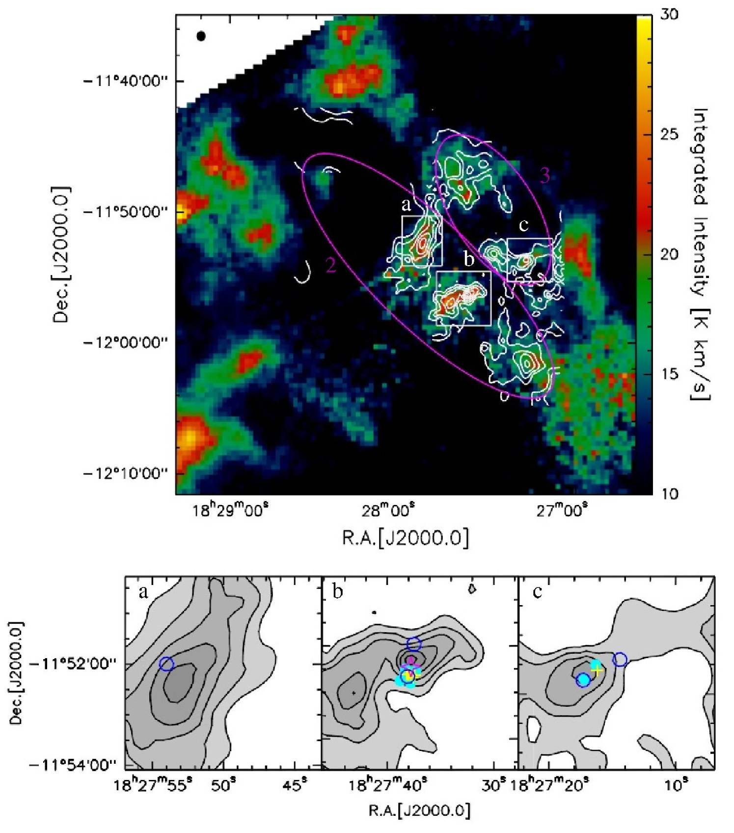
Figure 1: FCRAO velocity-integrated ¹³CO(1-0) emission in white contours from our data, overlaid on the ¹³CO(1-0) emission from the BU-FCRAO GRS (color). Both maps are integrated between 25 and 77 km s^-1. The contour levels range from 10 $\sigma$ in steps of 3 $\sigma$ ($\sigma$= 2 K km s^-1). The magenta ellipses represent: 1) the Giant Molecular Cloud (GMC) surrounding G19.61-0.23, which is the 32-50 km s^-1 molecular gas (cloud 2) discussed in Sect. 3.2; and 2) the 54-63 km s^-1 molecular gas (cloud 3) discussed in Sect. 3.2. The three white boxes, labelled as “a”, “b” and “c”, highlight the three regions displayed in the bottom part of the figure. The cyan filled circles represent the HII regions, the yellow crosses are the water masers, the magenta open stars are the OH masers and the blue open circles are the methanol masers (see Table 9).

This main cloud is also seen in the central region of the C¹⁸O(1-0) velocity-integrated map (available in Fig. 12 in the Online material Sect.), as well as in all other tracers of star formation, such as masers, HII regions and IR emission (see Table 9). A good correlation between the ¹³CO(1-0) and C¹⁸O(1-0) emission is seen also in the other two regions sampled in the C¹⁸O(1-0) line, which present the same morphology as the ¹³CO(1-0) emission.

3.1 A closer view of the molecular line emission

Observations of both transitions of all three CO isotopologues were performed only in the central region of about $4.\!\!^{\prime}7\times 3.\!\!^{\prime}6$ (17 pc $\times$ 13 pc), containing the main complex of the molecular emission. Figure 2 shows in the top panel the FCRAO ¹³CO(1-0), C¹⁸O(1-0) and C¹⁷O(1-0) maps, integrated between 32 and 50 km s^-1, in the central region covering the main cloud of the complex. The bottom panels of Fig. 2 give the IRAM-30m ¹³CO(2-1), C¹⁸O(2-1) and C¹⁷O(2-1) maps, integrated over the same velocity range.

Figure 2: Top: FCRAO emission maps, integrated between 32 and 50 km s^-1, of the central $4.\!\!^{\prime}7\times 3.\!\!^{\prime}6$ region. Left: ¹³CO(1-0) emission; the contour levels range from 10 $\sigma$ ($\sigma=1$ K km s^-1) in steps of 5 $\sigma$. The white crosses are the positions of the emission peaks of the two central clumps, which are labelled as “co1” and “co2” (see Table 3). Middle: C¹⁸O(1-0) emission; the contour levels range from 10 $\sigma$ ($\sigma=0.2$ K km s^-1) in steps of 5 $\sigma$. Right: C¹⁷O(1-0) emission; the contour levels range from 10 $\sigma$ ($\sigma=0.05$ K km s^-1) in steps of 5 $\sigma$. Bottom: IRAM-30m emission maps, integrated between 32 and 50 km s^-1, of the central 5$.\!\!^{\prime}$5$\times$5$.\!\!^{\prime}$5 region. Left: ¹³CO(2-1) emission; the contour levels range from 10 $\sigma$ ($\sigma=4$ K km s^-1) in steps of 5 $\sigma$. The white crosses are the same as before. Middle: C¹⁸O(2-1) emission; the contour levels range from 10 $\sigma$ ($\sigma=2$ K km s^-1) in steps of 5 $\sigma$. Right: C¹⁷O(2-1) emission; the contour levels range from 10 $\sigma$ ($\sigma=2.7$ K km s^-1) in steps of 5 $\sigma$.

In the ¹³CO(1-0) and C¹⁸O(1-0) emission maps, the molecular gas is concentrated within two main clumps (clump co1 and clump co2, see Sect. 4.1). This is not confirmed in the C¹⁷O(1-0) emission map, where the two peaks are not clearly distinguished. This is maybe affected by the low sampling of the region in the C¹⁷O(1-0) line. The same morphological characteristics are confirmed in the ¹³CO(2-1) line, where the two clumps can be clearly distinguished, and partially in the C¹⁸O(2-1) line, where clump co2 is still visible, although very faint. In the C¹⁷O(2-1) emission, clump co2 is even fainter and, due to the lower signal to noise radio, it is hard to be distinguished.

3.2 Kinematics of the emission and cloud definition

Figure 13, in the Online Material Sect., shows the large-scale channel maps of the ¹³CO(1-0) emission (i.e., the emission in 2 km s^-1 wide velocity intervals), which reveals the complex spatial and velocity structure of the molecular gas. The contours of the emission are from 10 $\sigma$ ($\sigma$ = 0.2 K per channel) in steps of 5 $\sigma$. The numbered crosses represent the molecular features (clumps), which we identified in the emission (see Sect. 4.1).

Throughout this paper we will use the word “cloud” for the four main molecular complexes described below and identified in the ¹³CO(1-0) emission and “clump” for the smaller scale structures resolved within the four main clouds (see Sect. 4.1).

We distinguish four velocity intervals, corresponding to the main features (clouds) that can be identified in the molecular gas. These are four molecular clouds, well separated in velocity and/or spatial distribution. The main parameters of these four molecular clouds are given in Table 2 and Fig. 3 shows the integrated emission from each of them.

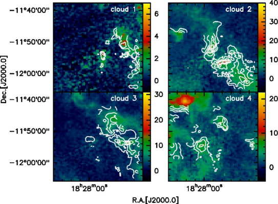
Figure 3: Maps of the four molecular clouds identified in ¹³CO(1-0) emission, integrated over the velocity channels of emission of each cloud (see col. 2 of Table 2). The FCRAO ¹³CO(1-0) emission from our data is represented by the white contours and is overlaid on the ¹³CO(1-0) emission from the BU-FCRAO GRS.

In particular, we identify:

Cloud 1

(28–32 km s^-1): the lowest velocity channels show no significant emission, with the exception of one narrow feature (clump co4, see Table 3), which is clearly visible above the 10 $\sigma$ level in the 29 km s^-1 velocity channel. In order to analyze this feature, we created a ¹³CO(1-0) data cube with a velocity resolution of 0.5 km s^-1.

Cloud 2

(32–50 km s^-1): this is the velocity range of the main complex of the emission, which is the GMC surrounding G19.61-0.23. It is represented by the larger magenta ellipse in Fig. 1, with linear semi-axes of 49 pc and 15 pc. All the emission is spatially concentrated in the same area, with an elliptical shape. This suggests that the emission is all at the same distance, i.e. at the distance of the main central region at 12.6 kpc. Several molecular features can be distinguished in the emission, both in the spatial and velocity distributions. The identification of the single clumps is discussed in Sect. 4; in particular, one of them, clump co5 (see Table 3) has been identified using the BU-FCRAO GRS, because it is at the edge of our observed region.

Cloud 3

(54–63 km s^-1): these velocity channels show several features in the emission as well, spread over 10 km s^-1. Also, in this case the emission is all concentrated in the same area, in the north-west of the sampled area, which suggests that it is all at the same distance. The smaller ellipse in Fig. 1 delineates the approximate outline of this GMC. It is worth noting that the narrow feature, seen only in the 60 km s^-1 velocity channel (clump co19, see Table 3), has been analyzed with the higher velocity resolution of 0.5 km s^-1.

Cloud 4

(64–73 km s^-1): the highest velocity channels show four main features in the emission and two of them (clump co14 and clump co17) have been identified using the BU-FCRAO GRS. The emission at the east edge of the map has not been included in the further analysis.

Both the near and far distances of each one of the four clouds have been computed, using the rotation curve of Brand & Blitz (1993). The derived distances as well as the galactocentric distances ($D_{\rm GC}$) are given in Table 2 for the four clouds identified in the FCRAO ¹³CO(1-0) emission, with the respective velocity interval of the emission.

Table 2: Summary of the parameters of the four molecular clouds identified in the FCRAO ¹³CO(1-0) emission.

Cloud	$\Delta$v	$d_{\rm FAR}$	$d_{\rm NEAR}$	$D_{\rm GC}$
	(km s-1)	(kpc)	(kpc)	(kpc)
(1)	(2)	(3)	(4)	(5)
1	28-32	13.4	2.6	6.1
2	33-48	12.6	3.4	5.4
3	54-63	11.7	4.3	4.7
4	64-73	11.3	4.7	4.3

• NOTES. – Col.(1): the cloud. Col.(2): the velocity interval of the emission. Col.(3): the far distance. Col.(4): the near distance. Col.(5): the galactocentric distance.

Finally, we point out that the association of the emission, which is close in velocity and position, as part of the same GMC is fairly arbitrary and has consequences for the distance estimates of the different clouds.

4 Identification of the clumps

4.1 The ¹³CO emission

Source identification was based on the visual inspection of all velocity channels of the FCRAO ¹³CO(1-0) map of the large-scale emission and of the BU-FCRAO GRS. The detection threshold used for the identification of the different clumps in the ¹³CO(1-0) emission was set to 10 $\sigma$ ($\sigma=0.2$ K). We identified 19 clumps in the FCRAO ¹³CO(1-0) emission, which are indicated in Fig. 13 (in the Online Material Sect.), in the channel corresponding to their peak emission (see also Table 3). The clumps co5, co10, co12, co11, co14 and co17, as shown in Fig. 13, are at the edges of the sampled region and we thus used the BU-FCRAO GRS data to derive their physical parameters for the analysis.

The angular extent of each identified clump was determined by finding the area, A_1/2, within the 50% intensity contour in the FCRAO ¹³CO(1-0) maps, integrated over the channels of the emission, and computing the equivalent radius of a circle with the same area. The angular diameter of each clump was derived by deconvolving the diameter, assuming source and beam to be Gaussian: thus $\Theta_{\rm S}=\sqrt{4A_{1/2}/\pi-\Theta_{\rm beam}^{2}}$. The derived angular sizes are given in Table 3. All the identified clumps have deconvolved sizes which are larger than the beam size of the observations, indicating that they are well resolved.

Table 3: Physical parameters of the clumps identified in the FCRAO ¹³CO(1-0) emission.

Clump	Peak Position		Velocity Range	$\Theta_{\rm S}$a	Tpeak	vpeak	FWHMb	$\int$T${}_{\rm B}{\rm dv}$	$d_{\rm FAR}$	$d_{\rm NEAR}$	$D_{\rm GC}$	${\frac{{}^{12}{\rm C}}{{}^{13}{\rm C}}}^{{\textsuperscript{e}}}$	${\frac{{}^{16}{\rm O}}{{}^{18}{\rm O}}}^{{\textsuperscript{e}}}$
	R.A.[J2000.0]	Dec.[J2000.0]	(km s${-1}$)	(arcsec)	(K)	(km/s)	(km/s)	(K km/s)	(kpc)	(kpc)	(kpc)
(1)	(2)	(3)	(4)	(5)	(6)	(7)	(8)	(9)	(10)	(11)	(12)	(13)	(14)
co1	18:27:37.63	-11:56:15.7	38–48	48.9	4.8	42.9	7.3	37.3	12.6	3.4	5.4	48.1	354.6
co2	18:27:43.21	-11:56:52.7	38–48	67.4	5.0	42.8	5.5	29.8	12.6	3.4	5.4	48.1	354.6
co3	18:27:51.73	-11:51:57.7	38–44	135.2	4.8	41.0	5.2	27.1	12.6	3.4	5.4	48.1	354.6
co4c	18:27:45.22	-11:53:18.7	28.5–29.5	75.6	3.9	28.8	0.8	3.9	13.4	2.6	6.1	53.4	395.8
co5d	18:28:25.15	-11:47:12.6	44–46	123.4	9.8	44.7	1.6	19.9	12.6	3.4	5.4	48.1	354.6
co6	18:27:17.01	-12:02:03.0	35–44	87.5	2.4	38.7	8.2	21.5	12.6	3.4	5.4	48.1	354.6
co7	18:27:17.03	-11:53:41.4	56–62	60.9	4.4	59.0	4.8	22.8	11.7	4.3	4.7	42.9	313.5
co8	18:27:29.61	-11:53:12.0	34–39	51.0	3.0	37.0	5.2	16.8	12.6	3.4	5.4	48.1	354.6
co9	18:27:22.07	-11:54:47.6	34–39	53.0	2.7	35.2	3.5	10.4	12.6	3.4	5.4	48.1	354.6
co10d	18:27:34.05	-11:45:26.1	54–62	135.9	2.5	57.4	6.5	17.2	11.7	4.3	4.7	42.9	313.5
co11d	18:27:24.62	-11:46:40.3	59–63	172.2	3.0	59.8	5.0	16.3	11.7	4.3	4.7	42.9	313.5
co12d	18:27:23.49	-11:49:08.2	56–59	49.6	2.7	58.2	5.7	16.9	11.7	4.3	4.7	42.9	313.5
co13	18:27:27.60	-11:53:19.2	56–60	90.3	3.7	57.6	4.1	16.3	11.7	4.3	4.7	42.9	313.5
co14d	18:28:18.23	-11:39:54.2	63–67	179.5	5.9	65.4	4.1	26.3	11.3	4.7	4.3	39.9	289.9
co15	18:27:35.66	-11:50:22.0	57–59	83.1	3.6	57.9	2.4	9.7	11.7	4.3	4.7	42.9	313.5
co16	18:27:41.68	-11:47:39.9	65–67	142.2	4.4	65.8	1.7	9.1	11.3	4.7	4.3	39.9	289.9
co17d	18:28:30.14	-11:41:02.6	69–72	217.2	4.1	69.1	3.4	15.5	11.3	4.7	4.3	39.9	289.9
co18	18:28:02.29	-11:54:25.9	69–73	99.4	2.5	71.0	4.5	12.3	11.3	4.7	4.3	39.9	289.9
co19c	18:27:28.11	-12:02:32.0	59.5–61	61.5	2.6	60.2	1.4	4.2	11.7	4.3	4.7	42.9	313.5

• NOTES. – Col.(1): Clump. Col.(2)-(3): Peak position of the emission. Col.(4): Velocity range of the clump emission. Col.(5): Deconvolved angular diameter of the clump. Col.(6): Peak T_mb of the spectrum. Col.(7): Peak velocity of the spectrum. Col.(8): Deconvolved FWHM line-width of the spectrum. Col.(9): Integrated intensity emission from the FWHM contour of the clump. Col.(10): Far distance of the clump. Col.(11): Near distance of the clump. Col.(12): Galactocentric distance of the clump. Col.(13): Carbon isotope ratio. Col.(14): Oxygen isotope ratio.

• Deconvolved for the beam size.

• Deconvolved for the velocity resolution.

• The parameters are derived from a high velocity resolution resample (0.5 km/s).

• The physical parameters are derived from the BU-FCRAO GRS data, because the clump is at the edge of our map.

• The carbon and oxygen isotope ratios have been obtained using: ${{}^{12}\rm C}/{{}^{13}\rm C}=7.5\,D_{\rm GC}+7.6$ and ${{}^{16}\rm O}/{{}^{18}\rm O}=58.8\,D_{\rm GC}+37.1$ (Wilson & Rood 1994), where $D_{\rm GC}$ is the galactocentric distance (col. 11).

As explained above, we computed both the near and far distances for each of the four velocity intervals of the emission, corresponding to the four main molecular clouds in the whole region. Therefore, assuming that each of the four molecular clouds is made from material at the same distance, which is reasonable given the localized morphology of the emission, each clump is assumed to be at the same distance as the cloud it belongs to (see Table 3). This leaves the question of the “near-far ambiguity”, which we discuss in Sect. 5.

The spectrum of the emission of each identified clump was obtained by integrating the ¹³CO(1-0) data cube in the channels of the emission of the clump, over the area enclosed by the deconvolved 50% contour level of the ¹³CO(1-0) emission. The spectra of clump co4 and clump co19 have been derived from the higher velocity resolution (0.5 km s^-1) data-cube, as discussed in the previous section. The parameters of each clump were determined by fitting a Gaussian profile to each produced spectrum. Line profiles showing more than one velocity component were analyzed by fitting more than one Gaussian component, in order to remove the contribution to the emission by other clumps along the line of sight from the emission coming from the clump of interest. The results of this analysis are reported in Table 3.

4.2 The continuum emission

Figure 4 shows the APEX 870 $\mu$m continuum emission from the same region we observed in the ¹³CO(1-0) emission line (see Fig. 1). The data are part of the ATLASGAL project (Schuller et al. 2009). The white ellipses represent: 1) the GMC surrounding G19.61-0.23, which is the 33–48 km s^-1 molecular gas (cloud 2) discussed in Sect. 3.2; and 2) the 54–63 km s^-1 molecular gas (cloud 3) discussed in Sect. 3.2 (see also Fig. 1).

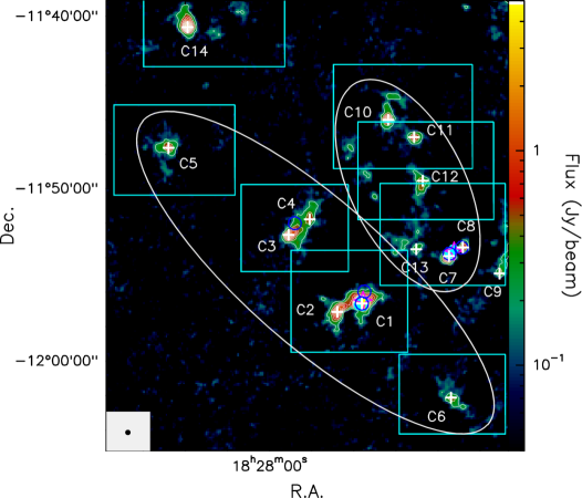
Figure 4: APEX 870 $\mu$m continuum emission. The contour levels are from 5 $\sigma$ ($\sigma=40$ mJy beam^-1) in steps of 5 $\sigma$. The label of each identified source is indicated and the positions of each emission peak is marked with a white cross. Symbols are as in Fig. 1 (see Table 9). The cyan boxes highlight the fields of Fig. 14. The white ellipses represent: 1) the GMC surrounding G19.61-0.23, which is the 33–48 km s^-1 molecular gas (cloud 2) discussed in Sect. 3.2; and 2) the 54–63 km s^-1 molecular gas (cloud 3) discussed in Sect. 3.2 (see also Fig. 1).

We decided to use a threshold of 10 $\sigma$ to identify the different sources in the continuum emission. In this way, we identified in the APEX continuum emission 14 sources, which are shown in Fig. 4 with their respective labels.

Most of the APEX continuum sources have counterparts in one of the FCRAO ¹³CO(1-0) clumps (see also Fig. 14 in the Online Material Sect.), with the exception of sources C8 and C9. Source C8 is associated with significant emission in the ¹³CO(1-0) line, but over a region slightly to the south of C8 (see Fig. 14). The ¹³CO(1-0) emission in this case corresponds to ¹³CO clump co7, which “contains” the APEX sources C8 and C7. We thus assume for both C8 and C7 the distance corresponding to ¹³CO 8. C9 is associated with ¹³CO emission at 62 km s^-1 and hence probably to cloud 3.

Table 4: Physical parameters of the sources identified in the APEX 870 $\mu$m continuum emission.

Source	Peak Position		$\Theta_{\rm C}$a	Fpeak	v${}_{{}^{13}{\rm CO}}$	Flux	Counterpart	$d_{\rm FAR}$	$d_{\rm NEAR}$	$M_{\rm cont}$b
	R.A.[J2000.0]	Dec.[J2000.0]	(arcsec)	(Jy/beam)	(km s-1)	(Jy)		(kpc)	(kpc)	($\times 10^{2}\,M_{\odot}$)
(1)	(2)	(3)	(4)	(5)	(6)	(7)	(8)	(9)	(10)	(11)
C1	18:27:38.05	-11:56:38.3	15.2	16.3	42.9	14.1	co1	12.6	3.4	203.4
C2	18:27:43.88	-11:57:07.9	36.9	1.4	42.8	3.6	co2	12.6	3.4	52.5
C3	18:27:55.43	-11:52:39.7	30.6	1.6	41.0	2.9	co3	12.6	3.4	42.1
C4	18:27:50.42	-11:51:45.7	38.1	0.7	41.0	1.7	co3	12.6	3.4	23.8
C5	18:28:23.88	-11:47:36.8	24.7	0.9	44.7	1.2	co5	12.6	3.4	17.1
C6	18:27:16.91	-12:02:06.3	32.8	0.5	38.7	1.1	co6	12.6	3.4	15.2
C7	18:27:17.36	-11:53:53.7	21.6	2.2	59.0	2.5	co7	11.7	4.3	31.5
C8	18:27:14.08	-11:53:23.5	20.5	0.8	57.7	0.9	-	11.7	4.3	11.1
C9	18:27:05.36	-11:54:54.3	29.0	0.4	62.5	0.8	-	11.6	4.4	9.5
C10	18:27:31.77	-11:45:59.5	20.5	1.5	57.7	1.7	co10	11.7	4.3	21.2
C11	18:27:25.62	-11:46:59.9	22.7	0.9	59.8	1.1	co11	11.7	4.3	13.5
C12	18:27:23.58	-11:49:31.7	45.4	0.5	58.2	1.9	co12	11.7	4.3	24.1
C13	18:27:25.13	-11:53:29.9	25.6	0.4	57.6	0.6	co13	11.7	4.3	7.3
C14	18:28:19.32	-11:40:37.2	27.4	2.4	65.4	3.8	co14	11.3	4.7	7.6

• NOTES. – Col.(1): Sources. Col.(2)-(3): Peak positions of the emission. Col.(4): Deconvolved angular diameters of the sources. Col.(5): Peak flux densities of the sources. Col.(6): Velocity of the sources from the association with the FCRAO ¹³CO(1-0) emission. Col.(7): Integrated emission from the FWHM contour of the sources. Col.(8): FCRAO ¹³CO(1-0) counterpart. Col.(9): Far distance of the source from the ¹³CO(1-0) emission (see Table 3). Col.(10): Near distance of the source from the ¹³CO(1-0) emission (see Table 3). Col.(11): Mass from the continuum emission of the sources, assuming $T=20$ K.

• Deconvolved.

• All the sources are assumed to be at the far kinematic distances, except C14 (see text).

Moreover, given the lower resolution of the ¹³CO data, the continuum sources C3 and C4 correspond both to clump co3 in the FCRAO ¹³CO(1-0) emission. Column 8 of Table 4 indicates the counterpart, if any, of each APEX continuum source, as identified from the comparison between the ¹³CO emission and the APEX continuum emission. It is worth noting that the two maps (¹³CO map and APEX continuum maps) have significantly different resolutions, with the APEX resolution being $18.\!\!^{\prime\prime}2$ at 870 $\mu$m and the FCRAO resolution being 46^′′ at the frequency of the ¹³CO(1-0) line. Therefore it is not surprising that the sources identified in the APEX continuum emission are more compact than the ¹³CO clumps (as seen also in Fig. 14). Moreover, the 870 $\mu$m continuum emission probably traces dense cores embedded in the ¹³CO(1-0) clumps.

For the APEX continuum sources that have a counterpart in the FCRAO ¹³CO(1-0) emission, we assume as distance the one of the corresponding ¹³CO(1-0) clump. The obtained distances are reported in col. 9-10 of Table 4 (see Sect. 4.1 and Table 3).

5 Association with infrared emission

One of our aims is to compare the properties of the molecular clumps with and without star formation within them. With this in mind, we have compared images from the GLIMPSE (Benjamin et al. 2003) and MIPSGAL mid infrared surveys (Carey et al. 2005) with both ATLASGAL maps and our FCRAO ¹³CO data (supplemented by the BU-FCRAO GRS). It is worth recalling that the MIPSGAL 70 $\mu$m survey has a “beam” of $18^{\prime\prime}$, which is comparable to that of ATLASGAL. Moreover, the GLIMPSE 8 $\mu$m data traces PAH emission excited by UV from OB stars close to GMCs whereas the 24 $\mu$m MIPSGAL radiation often traces dust heated by embedded proto-stellar objects. Also, the 4.5 $\mu$m GLIMPSE data has been found often to trace molecular hydrogen emission associated with outflows. In Fig. 14 (online version), we superpose FCRAO ¹³CO and ATLASGAL maps to Spitzer images at 3.6, 8 and 24 $\mu$m.

One sees here that there are several ATLASGAL sources associated with strong continuum emission in the Spitzer bands. Table 5 summarizes these associations (within 1^′) as well as the information about maser emission and HII regions close to the positions of continuum emission.

Table 5: Association (within 1^′) of the APEX 870 $\mu$m sources with active star-formation tracers, such as Spitzer 3.6 $\mu$m, 8 $\mu$m and 24 $\mu$m; water, methanol and OH masers; HII regions; and IRAS sources.

APEX	Spitzer			Masers			HII	IRAS
	3.6	8	24	H2O	OH	CH3OH
(1)	(2)	(3)	(4)	(5)	(6)	(7)	(8)	(9)
C1	+	+	+	+	+	+	+	+
C2	+	+	+	–	–	–	–	–
C3	+	+	+	–	–	+	–	+
C4	+	+	+	–	–	+	–	–
C5	+	+	+	–	–	–	–	–
C6	+	+	+	–	–	–	–	+
C7	+	+	+	–	+	+	+	+
C8	+	+	+	–	–	+	–	–
C9	+	+	+	–	–	–	–	–
C10	+	+	+	–	–	–	–	+
C11	+	+	+	–	–	–	–	–
C12	+	+	+	–	–	–	+	+
C13	+	+	+	–	–	–	–	–
C14	+	+	+	–	–	–	–	+

• NOTES. – The “+” symbol indicates that the association with the tracer has been observed; while the “–” symbol indicates that it has not been observed.

Not surprisingly, there is strong mid infrared emission from the vicinity of clumps C1 and C2 which are associated with the HII region complex G19.61-0.23 but one also notes strong emission associated with the C7/C8 complex and with C12. In all of these cases, it is reasonable to assume that there is an embedded cluster of young stars producing ultra–violet radiation responsible for exciting the PAH and small grain emission observed at 8 and 24 $\mu$m. Less obvious in Fig. 14 is the fact that in many cases there are point-like ($<$ 6 arc sec.) continuum sources at 24 $\mu$m close to the ATLASGAL 870 micron peaks. It is noticeable that there are 3 ATLASGAL sources without clear 24 $\mu$m counterparts and we presume this implies a relatively low dust temperature (below 25 K). These are perhaps similar to the infrared dark clouds (IRDCs) observed associated with star-forming regions closer to the sun but lacking a strong infrared background. We note also that we have searched without success for extended emission in the 4.5 $\mu$m IRAC band of the type often found associated with outflows in nearby star-forming regions. Finally, all the ATLASGAL sources show association with extended Spitzer 8 $\mu$m emission, except source C14, which corresponds to the ¹³CO clump co14, and the ¹³CO clump co17 (see Table 3). Both clumps correspond to IRDCs seen against the 8 $\mu$m emission and identified by Simon et al. (2006a, b).

The above information suggests to us that all the ATLASGAL clumps but C14 are at the “far” (around 12 kpc) distance rather than the near (around 4 kpc). This is likely to be true for the clumps with velocity around 42 km s^-1 (cloud 2 in the nomenclature of Table 2), as shown by Kolpak et al. (2003) and confirmed by Anderson & Bania (2009). We therefore use the far distance as a working hypothesis in what follows for all clumps, with the exception of continuum emission clump C14 and clumps co14 and co17, seen in ¹³CO(1-0) emission, for which we used the near distance.

We demonstrate the association between ATLASGAL sources and 24 $\mu$m MIPSGAL sources in Fig. 5 where we plot a histogram (upper panel) of the angular separations between the 870 $\mu$m peak and the nearest 24 $\mu$m source.

Figure 5: Top: Histogram of the distances of the APEX 870 $\mu$m continuum sources from the closest Spitzer 24$\mu$m sources. Bottom: Histogram of the average distribution of the distance from the closest Spitzer 24 $\mu$m source for ten random samples of positions within the whole $23^{\prime}\times 23^{\prime}$ region (see Fig. 1).

To estimate the reliability of the associations of the infrared sources with the millimeter continuum cores, we have simulated randomly located samples of 14 cores and associated them with the closest infrared source. The bottom panel of Fig. 5 shows the distribution of the average separation between the infrared sources and the random sample of millimeter cores. One sees that the histogram for the real millimeter cores has a strong peak for separations of less than 10^′′ (roughly half the APEX beam) which is not present for the random samples. A statistical test on the two histograms shows that there is only a $\sim$0.1% probability that they are drawn from the same parent distribution. Indeed, the simulation shows that one roughly expects 2 chance coincidence within 15^′′ whereas there are 11 APEX sources within 15^′′ of the nearest Spitzer 24 $\mu$m source. We thus conclude that, with the exception of the three sources with separations larger than 30^′′, the associations of the ATLASGAL 870 $\mu$m cores with their neighboring Spitzer 24 $\mu$m sources are real.

6 Physical parameters of the clumps

6.1 The ¹³CO(1-0) emission

The central $5.\!\!^{\prime}2\times 5.\!\!^{\prime}2$ is the only region where we have observations of the $J=1-0$ and the $J=2-1$ transitions of the three isotopologues and therefore the only region where we can derive the optical depth of the ¹³CO(1-0) line. The optical depth, $\tau_{\rm{}^{13}CO}$, of the ¹³CO(1-0) transition can be estimated from the line ratio of the two isotopes, ¹³CO(1-0) and C¹⁸O(1-0). We derive values for the mean line optical depth of $\leq 0.5$ suggesting that while the line peak may be moderately optically thick ($\tau_{\rm{}^{13}CO}\sim 1.4-1.6$ at most), the integrated ¹³CO(1-0) emission is optically thin over the central region. This is also consistent with the observed lack of variation of the integrated (2-1)/(1-0) line ratios, as a function of the integrated line intensities (Fig. 6). The points in the plots correspond to the values of the line ratios taken over 46^′′ beams.

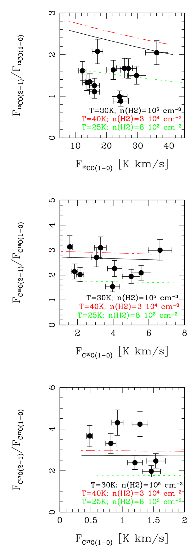
Figure 6: Integrated (2-1)/(1-0) line ratios over the central $4.\!\!^{\prime}7\times 3.\!\!^{\prime}6$ region as a function of the integrated line intensities, after smoothing the 30-m maps to the angular resolution of the FCRAO maps (46^′′). The points in the plots correspond to the values of the line ratios taken over 46^′′ beams. The curves are the theoretical curves from LVG models, correspondent to: $T=30$ K and n(H₂)=$10^{5}$ cm^-3 (black solid curve); $T=40$ K and n(H₂)=$3\,10^{4}$ cm^-3 (red dot-dashed curve); and $T=25$ K and n(H₂)=$8\,10^{3}$ cm^-3 (green dashed curve). Top: ratio between IRAM ¹³CO(2-1) emission and FCRAO ¹³CO(1-0) emission against the FCRAO ¹³CO(1-0) emission. Middle: ratio between C¹⁸O(2-1) emission and C¹⁸O(1-0) emission against the C¹⁸O(1-0) emission. Bottom: ratio between C¹⁷O(2-1) emission and C¹⁷O(1-0) emission against the C¹⁷O(1-0) emission.

Given that the ¹³CO emission at the peak of the line is close to be optically thick, as an estimate of the excitation temperature of the molecular gas we assumed 20 K, the peak line brightness temperature as measured in the clump with the highest optical depth. In the following we have assumed this excitation temperature for all the clumps.

The total column density of the ¹³CO molecule for each identified clump was derived using the $J=1-0$ transition, under the assumption of local thermodynamic equilibrium (LTE) at an excitation temperature $T_{ex}$. The column density of this molecule, in the optically thin limit, is given by

$$N_{{}^{13}{\rm CO}}=A\,\frac{T_{ex}+(h\,B_{\rm{}^{13}CO}/3\,k)}{e^{-h\nu_{\rm{}^{13}CO}/k\,T_{ex}}}\,\int T_{\rm B}{\rm dv}\,\,\,\,\,\,\,\,\,\,\,\,\,\,\,\,\,\,\,\,\mathrm{[cm^{-2}]}\\$$ (1)

where:

$$A=10^{5}\,\frac{3\,k^{2}}{8\,h\,\pi^{3}\,B_{\rm{}^{13}CO}\,\mu_{\rm{}^{13}CO}^{2}\,\nu_{\rm{}^{13}CO}}$$ (2)

(see Eq. [A1] and [A4] of Scoville et al. 1986). $\int T_{\rm B}{\rm dv}$ is the integrated line brightness temperature in K km s^-1 of the transition with frequency $\nu_{\rm{}^{13}CO}$ (Hz), $B_{\rm{}^{13}CO}$ is the rotational constant of the molecule and $\mu_{\rm{}^{13}CO}$ is ¹³CO’s permanent electric dipole moment, which is taken to be 0.1101 Debye. Assuming $T_{ex}=20$ K for every clump, we computed the total column density of each clump identified in the FCRAO ¹³CO(1-0) emission. The results are shown in col. 2 of Table 6.

The total LTE mass of gas in the identified clumps, $M_{\rm LTE}$, can be computed from the ¹³CO column density as follows:

$$M_{\rm LTE}=N_{\rm{}^{13}CO}\,\frac{[\rm H_{2}]}{[\rm^{13}CO]}\,\mu_{\rm G}\,m_{\rm H}\,\frac{\pi\,\Theta_{\rm S}^{2}}{4}\,d^{2}$$ (3)

(Scoville et al. 1986), where [H₂]/[¹³CO] is the abundance ratio of molecular hydrogen to ¹³CO, $\mu_{\rm G}=2.72$ is the mean molecular weight of the gas, $m_{\rm H}$ is the mass of the hydrogen atom, $\Theta_{\rm S}$ is the angular diameter of each clump (deconvolved FWHM, see col. 5 of Table 3) and $d$ is the distance of the source. Adopting an abundance ratio [H₂]/[¹²CO$]=10^{4}$ (e.g. Scoville et al. 1986), [H₂]/[¹³CO]=([H₂]/[¹²CO])$\times$([¹²C]/[¹³C]) can be computed for each clump, using the values of [¹²C]/[¹³C] presented in col. 13 of Table 3. We can thus derive the gas mass of each clump (col. 3 of Table 6).

Table 6: Masses and surface densities of the clumps identified in the FCRAO ¹³CO(1-0) emission.

Clump	$N_{{}^{13}{\rm CO}}$	$M_{\rm LTE}$c	$\Sigma_{\rm LTE}$	nLTEc	$M_{\rm VIR}$c	$\Sigma_{\rm VIR}$c	nVIRc
	($\times 10^{15}$ cm-2)	($\times 10^{2}\,M_{\odot}$)	(g cm-2)	($\times 10^{2}$ cm-3)	($\times 10^{2}\,M_{\odot}$)	(g cm-2)	($\times 10^{2}$ cm-3)
(1)	(2)	(3)	(4)	(5)	(6)	(7)	(8)
co1	47.5	34.6	0.10	37.2	164.9	0.49	177.1
co2	37.9	52.4	0.08	21.5	128.9	0.20	52.9
co3	34.5	192.3	0.08	9.8	230.9	0.09	11.7
co4a	4.9	10.8	0.01	2.6	3.2	0.003	0.8
co5b	25.4	117.6	0.06	7.9	20.3	0.01	1.4
co6	27.3	63.8	0.06	11.9	381.0	0.35	71.4
co7	29.1	25.2	0.06	17.5	83.5	0.19	58.0
co8	21.3	16.9	0.05	16.0	89.9	0.25	85.2
co9	13.2	11.3	0.03	9.5	41.1	0.10	34.7
co10b	22.0	94.9	0.04	5.9	342.7	0.15	21.4
co11b	20.8	144.3	0.04	4.4	251.6	0.07	7.7
co12b	21.5	12.4	0.04	15.9	96.0	0.32	123.4
co13	20.7	39.5	0.04	8.4	88.4	0.09	18.9
co14b	33.6	38.0	0.06	15.9	71.6	0.11	30.0
co15	12.3	19.9	0.02	5.5	27.6	0.03	7.5
co16	11.6	47.7	0.02	2.9	22.4	0.01	1.4
co17b	19.7	32.6	0.04	7.7	59.5	0.06	14.0
co18	15.7	31.5	0.03	5.6	117.2	0.11	20.8
co19a	5.3	4.7	0.01	3.2	7.6	0.02	5.1

• NOTES. – Col.(1): Clump. Col.(2)-(4): Column density, LTE mass and surface density for T${}_{ex}=20$ K. Col.(5) Density from the LTE mass. Col.(6)-(7): Virial mass and surface density. Col.(8) Density from the virial mass.

• The parameters are derived from a high velocity resolution resample (0.5 km/s).

• The values are derived from the BU-FCRAO GRS data, because the clump is at the edge of our map.

• All the clumps are assumed to be at the far kinematic distances, except clump co14 and clump co17.

The estimated gas masses can be compared with the masses computed under the assumption of virial equilibrium for an homogeneous sphere, neglecting contributions from the magnetic field and surface pressure:

$$M_{\rm VIR}=0.509\,d(\rm kpc)\,\Theta_{\rm S}(\rm arcsec)\,\Delta{\rm v_{1/2}}^{2}(\rm km\,s^{-1})$$ (4)

(e.g. MacLaren et al. 1988), where $\Delta{\rm v_{1/2}}$ is the ¹³CO(1-0) line width in kilometers per second and $\Theta_{\rm S}$ is the angular diameter of each clump in arcsec within the 50% intensity contour of the integrated ¹³CO(1-0) emission (see col. 5 of Table 3). The derived virial masses are presented in col. 6 of Table 6.

We also computed the surface density, $\Sigma$=M/($\pi$R²), of each clump, using both the LTE masses and the virial masses and they are given in col. 4 and col. 7 of Table 6, respectively. The surface density is a measure of pressure for virialized clouds, since the gas pressure needed to support a virialized cloud against gravity in the absence of other forces is of the order $G\,\Sigma^{2}$, independent of the shape of the cloud (e.g. McKee et al., 1993; Bertoldi & McKee, 1992). From Table 6, one sees that the surface densities derived from ¹³CO ($\Sigma_{\rm LTE}$), which are essentially distance independent, vary in the range 0.01 to 0.1 g cm^-2, which is roughly equivalent to a range of visual extinction 2.5 to 25 magnitudes for a local ISM dust-to-gas ratio. This is comparable to the surface density averaged over the whole cloud 2 GMC (see Table 8 and Sect. 9) and so these clumps are mostly at pressures of the order typically experienced in the GMC. The masses range from $3\,10^{2}$ to $2\,10^{4}\,M_{\odot}$ and thus overlap with the range studied by Williams & Blitz (1998) in the Rosette cloud and in G216-2.5.

For each clump we also derived an average density, using the deconvolved half power sizes we determined from the ¹³CO(1-0) emission (see col. 5 of Table 3). The values we obtained are reported in col. 5 and 8 of Table 6, respectively from the LTE masses and the virial masses, and are in the range $10^{2}$-$10^{4}$ cm^-3. These values can be compared with the results from LVG models, based on the approach of de Jong et al. (1975, spherically symmetric homogeneous model with linear dependence of $v$ upon $r$, collisional rates from ). Trapping has been accounted for using $N({\rm CO})/\Delta v$ as an independent variable where $N({\rm CO})$ can stand for any of the CO isotopologues of interest and we scale between them using the ratios given in Table 3 (line-width assumed to be the observed value of 5 km s^-1). In practice, trapping corrections are only of importance for ¹³CO and we find that the observed excitation, from the integrated (2-1)/(1-0) line ratios (see Fig. 6), is compatible with $T=30-40$ K and n(H₂)$=3\,10^{4}-10^{5}$ cm^-3 for the C¹⁸O and C¹⁷O lines and with $T=25-30$ K and n(H₂)$\lesssim 10^{4}$ cm^-3 for the ¹³CO line. The expected densities from LVG models are thus slightly larger than the average densities reported in Table 6. However, this can be explained with a moderate amount of clumping in the region.

6.1.1 The [¹⁸O]/[¹⁷O] ratio in G19.61-0.23

Using the FCRAO $J=1-0$ and IRAM $J=2-1$ data of C¹⁸O and C¹⁷O, we can derive the ¹⁸O/¹⁷O isotopic ratio in the central $5.\!\!^{\prime}2\times 5.\!\!^{\prime}2$ region centered on G19.61-0.23. Assuming that the two isotopologues have the same excitation temperature and that C¹⁸O is optically thin, we derive an average ¹⁸O/¹⁷O isotopic ratio of $4.2\pm 0.9$ for clump co1 and $3.9\pm 0.9$ for clump co2, from the line integrated intensity ratio between the FCRAO $J=1-0$ transitions of C¹⁸O and C¹⁷O, and of $3.0\pm 0.7$ for clump co1 and $3.0\pm 0.8$ for clump co2, from the line ratio between the IRAM $J=2-1$ transitions of C¹⁸O and C¹⁷O.

The values that we find are marginally consistent with the value discussed by Wilson & Rood (1994), $3.2\pm 0.2$. Moreover, we find a quite constant isotope ratio over the central region, including clump co1 and clump co2, in both transitions.

6.1.2 CO selective photodissociation

Figure 7 shows the line ratios for the CO isotopes for the central region of our map, as a function of the inferred H₂ column density. The points in the plots correspond to the values of the line ratios taken over every beam. At high values of line intensity (high column density), we do not see a variation of the line ratios. This is consistent with the fact that the integrated line intensities are mostly optically thin. At low column densities, there is a tendency of an increase of the ¹³CO(1-0)/C¹⁸O(1-0) ratio, which is also seen in the ratio of the (2-1) lines. This trend is consistent with the expectations for selective photodissociation at the edges of the clouds (see e.g. van Dishoeck & Black 1988).

Figure 7: The points in the plots correspond to the values of the line ratios taken over every beam, in regions of the map with high enough S/N ratio (larger than 5). Top left: ratio between FCRAO ¹³CO(1-0) emission and C¹⁸O(1-0) against H₂ column density derived from the C¹⁸O(1-0) line intensity. Top right: ratio between IRAM ¹³CO(2-1) emission and C¹⁸O(2-1) against H₂ column density derived from the C¹⁸O(2-1) line. Bottom left: ratio between FCRAO C¹⁸O(1-0) emission and C¹⁷O(1-0), against H₂ column density derived from the C¹⁸O(1-0) line intensity. Bottom right: ratio between IRAM C¹⁸O(2-1) emission and C¹⁷O(2-1) against H₂ column density derived from the C¹⁸O(2-1) line.

The enhancement in the ¹³CO/C¹⁸O ratio which we find is roughly a factor 1.5 in the FCRAO $J=1-0$ data, for A${}_{\rm V}\sim 6$ and N(H${}_{2})\sim 10^{21}$ cm^-2. This can be compared with the results of van Dishoeck & Black (1988) (see Table 7) for A${}_{\rm V}=9$, $T=30$ K, n${}_{\rm H}=2000$ cm^-3 and high UV field, which predict an enhancement of 1.7. We thus find that it is reasonable to assume that the trend that we find in the ¹³CO(1-0)/C¹⁸O(1-0) ratio at low column densities is due to selective photodissociation.

6.2 The continuum emission

To derive the angular extent of each identified source, we used the same method as described in Sect. 4.1 for the FCRAO ¹³CO(1-0) emission. The derived angular sizes, $\Theta_{\rm C}$, are shown in Table 4 (col. 4). As already pointed out in Sect. 4.2, all the continuum sources that have a ¹³CO counterpart (see column 8 of Table 4) have smaller sizes than the respective ¹³CO clumps. This is possibly indicating that the continuum sources trace the densest cores within the CO clumps. The integrated flux densities of the continuum sources are given in column 7 of Table 4.

Dust emission is generally optically thin in the sub-millimeter continuum. Therefore, following Hildebrand (1983) and assuming constant gas-to-dust mass ratio equal to 100, optically thin emission and isothermal conditions, the total gas+dust mass of each source is directly proportional to the continuum flux density integrated over the source:

$$M_{\rm cont}=\frac{F_{\nu}\,d^{2}}{\kappa_{\nu}\,B_{\nu}({\rm T})}$$ (5)

where $F_{\nu}$ is the integrated flux, $\kappa_{\nu}$ is the dust absorption coefficient per gram of gas, $B_{\nu}({\rm T})$ is the Planck function calculated at the dust temperature $T$ and $d$ is the distance of each source. Adopting a dust absorption coefficient $\kappa_{\nu}=\kappa_{0}\,(\nu/\nu_{0})^{\beta}$, with $\kappa_{0}=0.005$ cm² g^-1 at $\nu_{0}=230$ GHz (e.g. Hildebrand 1983; André et al. 2000) and $\beta=2$ (Hildebrand 1983), we derive $\kappa_{\nu}=0.0112$ cm² g^-1 at $\nu=870$ $\mu$m. For a dust temperature $T=20$ K, the derived masses for each continuum source are given in Table 4, col. 11. The masses range from 700 to $2\,10^{4}\,M_{\odot}$ and are similar to results for the ¹³CO, though the continuum sources are more compact.

7 Stability of the clumps

Figure 8 shows the ratio between the virial mass and the ¹³CO LTE mass for each of the 19 clumps identified in the FCRAO ¹³CO(1-0) emission, assuming the far distance for all clumps but clump co14.

Figure 8: Plot of the ratio between the mass derived assuming virial equilibrium ($M_{\rm VIR}$) and the LTE mass for the each clump ($M_{\rm LTE}$). The numbers on the x-axis correspond to the CO clumps, according to col. 1 of Table 3. Filled triangles indicate clumps associated with active star-formation tracers (see Table 5) and empty squares represent clumps which are not associated with star-formation tracers. The straight line corresponds to $M_{\rm VIR}=M_{\rm LTE}$.

The filled triangles indicate the clumps associated with active star-formation tracers (see Table 5) and the empty squares represent the clumps without star-formation tracers. The ratio is larger than 1 for all the sources but 3 (clumps co4, co5 and co16), which indicates that the clumps range from gravitational unbound to unstable in few cases, with an average value for the ratio of about 3. Most of the clumps thus seem to be transient molecular structures, as highlighted from the ¹³CO(1-0) analysis. This result does not seem to depend on whether the clumps are associated with star formation (see however Williams & Blitz 1998; Williams et al. 1995).

We can compare this result with the study of Fontani et al. (2002), who observed the molecular clumps associated with 12 ultracompact (UC) HII regions in CH₃C₂H and found that the clumps are unstable against gravitational collapse (see also Cesaroni et al. 1991 and Hofner et al. 2000 for the C³⁴S and the C¹⁷O lines). However, G19.61-0.23, also studied by Fontani et al. (2002), is one of only two sources with $M_{\rm VIR}/M_{\rm gas}$ ratio very close to one. Therefore, in order to investigate the discrepancy between Fontani et al. (2002) and us, we repeated the analysis using the C¹⁷O(2-1) from our IRAM-30m observations, for the two central clumps co1 and co2. We find for both clumps a much smaller $M_{\rm VIR}/M_{\rm LTE}$ ratio, which is $<1$ for clump co2. We thus find evidence that the $M_{\rm VIR}/M_{\rm LTE}$ ratio changes with the tracer: the gas traced by the ¹³CO seems to be more virialized than the gas traced by the C¹⁷O. Since C¹⁷O (as well as C³⁴S and CH₃C₂H) traces higher density gas than ¹³CO, our result seems to indicate that the clumps are globally in equilibrium but locally unstable. New observations of all the identified clumps in high density tracers are needed to further investigate this point.

It is worth to further discuss clump co5, which corresponds to continuum emission source C5, an interesting case because of its small virial mass compared with its LTE mass. From Fig. 8, the clump seems not to be in virial equilibrium against gravitational collapse. Moreover, it appears also to be associated with active star formation (see Fig. 14 and Table 5), which excludes the possibility that we overestimated the temperature in computing the LTE mass of the clump, from Eq.(3). A possible explanation for the small ratio $M_{\rm VIR}/M_{\rm LTE}$ of clump co5 is that the magnetic field might be playing an important role in stabilizing the clump.

It is also interesting to compare the continuum masses (column 10 of Table 4) of all the continuum sources that have a ¹³CO counterpart with the LTE masses of the respective ¹³CO clumps (column 4 of Table 6). All the continuum sources with a ¹³CO counterpart have $M_{\rm LTE}\succsim M_{\rm cont}$, which is probably due to the fact that the ¹³CO clumps have larger sizes than the respective continuum counterparts. However, there are three exceptions: the continuum source C1, which is associated with ¹³CO clump co1; the continuum source C7, which is associated with ¹³CO clump co7; and the continuum source C12, which is associated with ¹³CO clump co12. A possible explanation might be that we underestimated the temperature for these three sources, therefore we overestimated the continuum mass and we underestimated the LTE mass. This explanation is consistent with the association of the three sources with active star-formation tracers, in particular with Spitzer emission at 3.6 $\mu$m, 8 $\mu$m and 24 $\mu$m. Therefore we obtain the same result on the gravitational stability of the clumps also from the continuum masses.

8 SED and luminosities

In Sect. 5 we demonstrated that associations between the ATLASGAL sources and the 24 $\mu$m MIPSGAL emission exist. In the following we assume that these associations indeed are real and combine the Spitzer and APEX results in order to derive crude spectral energy distributions from the 24 and 70 $\mu$m MIPSGAL data and ATLASGAL 870 $\mu$m observations.

We have integrated the MIPSGAL 24 and 70 $\mu$m images over the area of ATLASGAL sub-mm continuum emission in order to derive the spectral energy distributions shown in Fig. 9.

Figure 9: Spectral energy distributions (SEDs) of the APEX 870 $\mu$m continuum sources that are associated with Spitzer 24 $\mu$m emission (see Sect. 5). The SEDs, shown as solid lines, are derived from fitting the 870 and 70 $\mu$m points with a modified black body of given density, dust temperature, and radius (see text for the details). The continuum sources C6, C9 and C12 are not presented in the plot because they do not seem to be directly associated with Spitzer 24 $\mu$m emission and the continuum source C1 has been excluded as well because its emission at 24 $\mu$m and 70 $\mu$m is saturated.

The Spitzer counterparts of ATLASGAL sources are mostly close to point-like (6^′′ at 24 $\mu$m and 18^′′ at 70 $\mu$m), thus more compact than the ATLASGAL sources, as one would expect for dust heated by a central object. We clearly do not have sufficient frequency coverage to get a precise estimate of the luminosity but we have derived crude estimates by fitting the 870 and 70 $\mu$m points with a modified black body of given density, dust temperature, and radius. This is not unique and always underestimates the 24 $\mu$m flux. However, it gives a reasonable first guess to the dust temperature appropriate for the ATLASGAL data and hence for the determination of the mass associated with the 870 $\mu$m emission. Results for the 10 sources fitted in this way are given in Table 7 and are shown in Fig. 9.

Table 7: Properties of the ATLASGAL sources with a counterpart in the mid-infrared emission, derived by fitting the 870 and 70 $\mu$m points with a modified black body.

Source	Radius	$d$a	F24μm	F70μm	Td	L	M	$\Sigma$
	(pc)	(kpc)	(Jy)	(Jy)	(K)	($\times 10^{4}\,L_{\odot}$)	($\times 10^{2}\,M_{\odot}$)	(g cm-2)
(1)	(2)	(3)	(4)	(5)	(6)	(7)	(8)	(9)
C2	0.7	12.6	7.6$\pm$1.5	119.8$\pm$24.0	25	5	60	0.81
C3	0.7	12.6	4.0$\pm$0.8	68.8$\pm$13.8	25	3	30	0.41
C4	0.7	12.6	2.1$\pm$0.4	42.8$\pm$8.6	27	2	10	0.14
C5	0.7	12.6	3.8$\pm$0.8	29.0$\pm$5.8	26	1	10	0.14
C7	0.7	11.7	9.1$\pm$1.8	107.3$\pm$21.5	28	3	20	0.27
C8	0.7	11.7	7.2$\pm$1.4	94.2$\pm$18.8	33	2	6	0.08
C10	0.7	11.7	–	100.6$\pm$20.1	29	3	10	0.14
C11	0.7	11.7	6.8$\pm$1.4	51.4$\pm$10.3	28	2	9	0.12
C13	0.6	11.7	2.6$\pm$0.5	72.0$\pm$14.4	32	1	4	0.07
C14	0.5	4.7	5.1$\pm$1.0	17.8$\pm$3.6	20	0.3	9	0.24

• NOTES. – Col.(1): ATLASGAL continuum source. Col.(2): radius of the APEX continuum source. Col.(3): distance of the source. Col(4): flux density at 24 $\mu$m of the IR source associated with the ATLASGAL 870 $\mu$m source. Col.(5): flux density at 70 $\mu$m of the IR source associated with the ATLASGAL 870 $\mu$m source. Col.(6)-(8): output of the modified black body fit. In particular: the dust temperature; the luminosity; the mass; and the surface density.

• All the sources are assumed to be at the far kinematic distances, except C14.

For the grey body fits we derive dust temperatures of 20–33 K and luminosities of 3000–50000 $L_{\odot}$, with corresponding gas masses of 10²–10⁴ $M_{\odot}$ and typical surface densities of 0.07–0.8 g cm^-2. So the results are in the range of values expected for young high mass (proto-)stars (e.g. Molinari et al. 2008).

One useful application of these results is to consider the inferred luminosity to gas mass ratio, $L/M$, for the ATLASGAL sources. This is a distance independent parameter and hence useful for comparison with extragalactic star-formation indicators (see Plume et al. 1992, 1997). Since bolometric luminosity is a rough measure of star formation rate (for a given initial mass function, IMF), $L/M$ is a measure of the gas exhaustion timescale of the clumps, which is typically much larger than the free fall time (see Krumholz & McKee 2005); hence, an indicator of the clump evolutionary timescale. One might expect $L/M$ to correlate with the surface density $\Sigma$ (also a distance independent quantity roughly speaking and a measure of pressure for virialized clumps) and we thus show in Fig. 10 a plot of $L/M$ against $\Sigma$  for our sample.

Figure 10: Luminosity to mass ratio, $L/M$, for the 870 $\mu$m continuum sources associated with the Spitzer emission at 24 $\mu$m (see Table 7), as a function of (1) the surface density, $\Sigma$ (left panel); (2) the mass (middle panel); and the luminosity (right panel). We note that source C14 is the only source at the “near” kinematic distance (see Table 7).

One expects $L/M$ to increase with time as molecular gas is converted into stars as star formation proceeds. One might also expect star formation rates to increase in regions of high pressure or surface density. It is interesting in this context that Sridharan et al. (2002) find evidence of an increase of $L/M$ going from regions without 3.6 cm radio emission (at the mJy level with the VLA) and clumps associated with UC HII regions. It would be useful to test this result for more homogeneous samples similar to the present one. We note, however, that Faúndez et al. (2004) find such result marginal and offer an alternative interpretation of $L/M$ as an indicator of the luminosity of the most massive star embedded within the clump. However, these results are based on much less sensitive radio continuum measurements, using a highly inhomogeneous sample of objects with distances varying over an order of magnitude. It is clear that larger samples with both high angular resolution far-infrared measurements and sensitive radio observations are needed to make further progress in this area.

A surprising feature of our results (see Fig. 10) is that low column density sources (below 0.5 g cm^-2) appear to have higher $L/M$ than high column density sources, which is hard to understand theoretically. However, this finding is marginal given the poor statistics.

These estimates for $L/M$ can be compared with the results of Wu et al. (2005) who used HCN as a dense gas tracer in order to estimate the star forming efficiency both in Galactic cores and extragalactic star-forming regions. From a survey of 31 Galactic cores, one can derive a median $L/M$ ratio of 63 L_⊙/M_⊙ for regions with luminosities above $3\,10^{4}\,L_{\odot}$; the ratio for extragalactic star-forming regions is similar. Below $3\,10^{4}\,L_{\odot}$, the ratio drops rapidly. Our median value of $L/M$ from the black body fit is roughly a factor of 4 lower but our sample is small and straddles the $3\,10^{4}\,L_{\odot}$ limiting value for the Wu et al. (2005) relation. However, given both the dispersion in the Wu et al. (2005) result and the uncertainties in our determinations of both L and M, we conclude that one needs both more complete SEDs and more reliable mass determinations to make further progress. The former will be undertaken by future surveys with HERSCHEL (such as HI-GAL; Molinari et al. 2010) but the latter will require careful calibration and intercomparison of the various approaches to determining clump masses.

9 Comparison with extragalactic observations

G19.61-0.23 is one of the most luminous ($\sim$2$\times 10^{6}\,L_{\odot}$, see Sect. 1) known Galactic massive star-forming regions and therefore one of the best templates to study locally the starburst phenomenon. Several high resolution studies have been carried out in this region as well as in other well known Galactic high mass star-forming regions. However, the aim of this work is to analyze the large-scale properties and physical conditions of the molecular gas in the region and the implications for extragalactic studies of nearby starburst galaxies.

Of particular interest are the youngest extragalactic embedded super star clusters (SSCs), which have been seen in merging systems (e.g. Whitmore 2002) and in some dwarf irregular galaxies (e.g. Elmegreen 2002; Johnson & Kobulnicky 2003) and have been identified by the free-free radio emission from their associated HII regions (e.g. Johnson & Kobulnicky 2003). One can see that the molecular clouds associated with the SSCs show lower surface densities than their end product (the star clusters). Since extragalactic studies are mostly done with single-dish telescopes and in low J transitions of CO, this result may be due to: (1) the limited linear resolution reached with current facilities; and/or (2) the molecular tracers used in the extragalactic studies, which are not tracing the real active sites of cluster formation, but rather lower density associated material.

In order to analyze the effect of low angular resolution in extragalactic studies, we compared the results from our ¹³CO low resolution observations of the Galactic region G19.61-0.23 with the physical parameters that have been found for some nearby extragalactic starbursts, in particular with CO(2-1) high angular resolution observations of Henize 2-10, a dwarf irregular starburst galaxy at the distance of 9 Mpc ($H_{0}$=75 km s^-1 Mpc^-1, Vacca & Conti 1992; Kobulnicky & Johnson 1999). We observed Henize 2-10 (Santangelo et al. 2009) at high angular resolution (1$.\!\!^{\prime\prime}9\times 1.\!\!^{\prime\prime}3$, which corresponds to a linear resolution of $80\times 60$ pc at the distance of Henize 2-10), revealing a rich population of molecular clouds with estimated masses and surface densities systematically larger than those measured in our Galaxy and we found possible evidence that the super star clusters are associated with very massive and dense molecular cores. We also compared our results with studies of M31 and M33 from Sheth et al. (2008) and Rosolowsky et al. (2003). They present CO(1-0) observations of the two spiral galaxies made with the BIMA array at a linear resolution of $\sim 20$ pc.

9.1 The total ¹³CO(1-0) emission

The total region of G19.61-0.23 that we sampled in ¹³CO(1-0) with FCRAO is about $27^{\prime}\times 27^{\prime}$ large (using the data from the BU-FCRAO GRS to cover the regions which were not sampled by our observations), which corresponds approximately to a size of 98 pc at the distance of the main complex of G19.61-0.23 (12.6 kpc). This value corresponds approximately to the size of each cloud identified in the SMA CO(2-1) emission of Henize 2-10 (see Table 8 and Table 3 of Santangelo et al. 2009). We can thus compare the properties of the total FCRAO ¹³CO(1-0) emission from the main cloud of the complex, containing G19.61-0.23 (cloud 2; see Sect. 3.2 and Table 2), with the physical parameters of the 14 clouds resolved in the SMA CO(2-1) emission from Henize 2-10.

With this aim, we analyzed the total FCRAO ¹³CO(1-0) emission from cloud 2 as if we were observing a single molecular cloud at the same linear resolution with which we observed Henize 2-10 ($\sim 80\times 60$ pc). In particular, we integrated all the ¹³CO(1-0) emission from the BU-FCRAO GRS data of cloud 2, between 32 and 50 km s^-1 and smoothed the derived spectrum to the same velocity resolution obtained in the SMA observations of Henize 2-10 (5 km s^-1). The physical parameters of cloud 2 “observed” in this fashion are given in Table 8, where the FWHM line width is listed in col. 1. We list, for comparison, in Table 8 also the parameters of one of the clouds resolved in the SMA emission from Henize 2-10.

Table 8: Summary of the parameters of the total integrated ¹³CO(1-0) emission of the GMC surrounding G19.61-0.23 and of a typical cloud in Henize 2-10, from SMA observations.

FWHM	$M_{\rm VIR}$	$M_{\rm LTE}$	$\Sigma_{\rm VIR}$	$\Sigma_{\rm LTE}$
(km/s)	($\times 10^{5}\,M_{\odot}$)	($\times 10^{5}\,M_{\odot}$)	(g/cm2)	(g/cm2)
(1)	(2)	(3)	(4)	(5)
G19.61-0.23
8	5	4	0.02	0.02
Henize 2-10
20	39	30	0.13	0.10

• NOTES. – Col.(1): FWHM line-width of the emission. Col.(2): Virial mass. Col.(3): LTE mass, assuming T_ex=20 K. Col.(4): Surface density from the virial mass. Col.(5): Surface density from the LTE mass.

We note that the line-widths (col. 1) are computed from the original total integrated ¹³CO(1-0) spectrum, before smoothing to the resolution of 5 km s^-1, and that the total emission is computed by integrating the emission from the channels relative to the emission from cloud 2 (between 32 and 50 km s^-1). From the comparison with the typical line widths of the clouds identified in Henize 2-10 (see Table 8), cloud 2 has a line width a factor of 2-3 smaller than the extragalactic clouds.

Following the same approach described in Sect. 6.1, we computed the virial mass and the LTE mass of cloud 2, assuming that: (1) the ¹³CO(1-0) emission is optically thin, as for the extragalactic clouds; (2) the cloud is at a distance of 12.6 kpc; and (3) T${}_{ex}=20$ K. We also computed the surface density of the cloud, using both the virial mass and the LTE mass. A summary of the derived masses and surface densities of cloud 2 is given in Table 8. The derived masses are smaller than the masses derived for the CO clouds in Henize 2-10, which are of the order of a few 10${}^{6}\,M_{\odot}$.

In Fig. 11 we show our results from Table 6 and Table 8 on a mass-surface density plot similar to that discussed by Tan (2007).

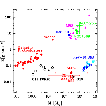
Figure 11: Surface density, $\Sigma=M/(\pi R^{2}$), versus mass, $M$, for star clusters and interstellar clouds. Several massive clusters are indicated: the pink triangles represent the SSCs in M82 (McCrady & Graham, 2007); the green circles are the SSCs in NGC 1569 (de Marchi et al., 1997; Larsen et al., 2008; Grocholski et al., 2008); and the green pentagon represents the cluster in NGC 5253 (McKee & Tan, 2003). Filled circles are star-forming clumps (Mueller et al. 2002). The typical GMC parameters are shown (Solomon et al. 1987). The values for M31 (Sheth et al. 2008) and M33 (Rosolowsky et al. 2003) are shown in red asterisks in the bottom right part of the diagram. The points labelled as He2-10 SMA are the clouds in Henize 2-10 from Santangelo et al. (2009), where the cyan points are computed from the virial masses and the blue points are computed from the molecular gas masses. The points labelled as G19 FCRAO are the clumps in G19.61-0.23 from this work, computed from the LTE masses. Finally, the point labelled as G19 represents the total emission from cloud 2 (see Table 8), computed from the LTE mass.

The blue and cyan squares are the values for the clouds in Henize 2-10, respectively, from the molecular and virial masses, which are in the same general area of the diagram as Galactic GMCs, though with somewhat higher masses and surface densities. Moreover, due to our limited angular resolution, the surface density may well be considerably underestimated. The black star represents the position of cloud 2 from the LTE mass (see Table 8). This cloud appears in the same area as the Galactic GMCs and the GMCs in M31 and M33, which confirms that there are no significant differences in the cloud properties of the two nearby spiral galaxies and the Milky Way (e.g. Rosolowsky et al. 2003; Sheth et al. 2008). However, cloud 2 shows lower surface density than the clouds in Henize 2-10, which suggests that the clouds in Henize 2-10 might be different from the GMCs in the Galaxy as well as from those in M31 and M33. Finally, the black circles represent the position in the plot for the clumps resolved in cloud 2 (clumps co1, co2, co3, co6, co8, co9 and co5), from the LTE masses. It is evident from the plot that the clumps resolved in cloud 2 have higher pressure than the whole molecular cloud 2, seen at low angular resolution. In particular, from the whole mass and surface of cloud 2 and the masses and surface of the clumps resolved in the ¹³CO(1-0) emission from cloud 2, we can derive a filling factor in area and in mass for the dense molecular gas in the GMC of G19.61-0.23, computed respectively as: $\sum_{i}\,A_{i}/A_{TOT}$ and $\sum_{i}\,M_{i}/M_{TOT}$, where $A_{i}$ and $M_{i}$ are the area and mass of every clump resolved in cloud 2 (i.e. clumps co1, co2, co3, co6, co8, co9 and co5; see Table 6) and $A_{TOT}$ and $M_{TOT}$ are the area and mass of cloud 2 (see Table 8). We find that the fraction of dense molecular gas in cloud 2 is about 10-20% (respectively from the LTE and the virial masses). Extrapolating those results to the extragalactic context, assuming that the fraction of the area and the mass of a GMC which is in the form of dense gas is the same as in the Galactic context, we would expect each cloud identified in Henize 2-10 to be resolved in several molecular clumps which account for a total dense molecular gas mass up to 10${}^{6}\,M_{\odot}$, each having a surface density up to 1.5 g cm^-2. It seems thus reasonable to assume that the clusters in Henize 2-10 form from small parsec sized clumps at much higher surface density and pressure than the rest of the GMC and than the typical Galactic clumps.

Therefore, we suggest that finding molecular clouds in Henize 2-10 with lower surface densities than their end product, the SSCs, might be due to the low linear resolution which is currently available. High sensitivity observations at higher resolution are needed to confirm this scenario, as well as observations of higher density tracers.

10 Summary and conclusions

In this paper we have presented single dish observations of the molecular gas and the sub-mm continuum of the high-mass star-forming region G19.61-0.23. Our observations, with a spatial resolution of about 2.8 pc at the adopted distance of 12.6 kpc, reveal a population of molecular clumps. The physical parameters of the identified clumps show a spread of virial parameters $M_{VIR}/M$, ranging from gravitationally unstable to unbound. These results seem to be independent of the presence or otherwise of star-formation indicators in the cloud, which is in slight contrast to results for less distant GMCs (e.g. Williams et al. 1995; Williams & Blitz 1998). One needs however more precise mass determinations for the clumps in G19.61-0.23, using high density molecular tracers, such as CS. Analogously, it would be very useful to obtain molecular line data for the ATLASGAL continuum sources.

Towards the ATLASGAL continuum sources, we have studied the association with mid-infrared emission and found that most ATLASGAL sources have counterparts in the mid-infrared emission at the peaks of the sub-millimeter continuum emission. For those sources we derived crude spectral energy distributions and estimated the luminosities and dust temperatures. We find that the majority of the continuum sources are associated with star-forming regions of luminosity 1–5 $10^{4}\,L_{\odot}$ and gas masses 400–6000 $M_{\odot}$. The luminosity to gas mass ratio, $L/M$, is in the range 10–100 $L_{\odot}/M_{\odot}$ with some evidence for a fall off for high mass clumps. The ATLASGAL sources are clearly good tracers of star formation.

We compared our results for the Galactic luminous high-mass star-forming region G19.61-0.23 with a previous extragalactic study of a dwarf starburst galaxy Henize 2-10. We find that the main cloud in G19.61-0.23 has physical properties comparable with the typical galactic GMCs and with the GMCs in M31 and M33. However this cloud shows less extreme properties than the clouds identified in Henize 2-10, in particular smaller surface densities and masses.

The new generation of telescopes is needed to address these questions. They will also allow to observe with higher sensitivity higher density tracers, to see the real sites of active star formation.

Appendix A Online material

In this appendix we present additional material, which may be useful. In particular, we show the list of all the sources in the sampled field, from the SIMBAD Astronomical Database (Table 9); the integrated intensity map of the C¹⁸O(1-0) emission from our FCRAO observations (Fig. 12); the channel map of our FCRAO ¹³CO(1-0) data (Fig. 13); and finally the overlay between the ¹³CO(1-0) clumps and the APEX continuum clumps with the Spitzer emission at 3.6, 8 and 24 $\mu$m (Fig. 14).

Table 9: List of the sources in the sampled field, from the SIMBAD Astronomical Database. Col.(1)-(2): Coordinates (J2000.0). Col(3): Distance from the peak emission of the associated clump (see Sect. 4.1). Col.(4): References.

Position		Distance	Ref.	Position		Distance	Ref.
R.A[J2000.0]	Dec.[J2000.0]	(arcsec)		R.A[J2000.0]	Dec.[J2000.0]	(arcsec)
(1)	(2)	(3)	(4)	(1)	(2)	(3)	(4)
HII Regions				H2O Masers
18:27:38.29	-11:56:29.4	16.8	1	18:27:38.00	-11:56:36.0	21.0	13
18:27:37.34	-11:56:32.4	17.2	2,3,7	18:27:37.80	-11:56:37.0	21.5	13
18:27:37.30	-11:56:32.3	17.3	1	18:27:38.00	-11:56:37.0	22.0	13
18:27:38.20	-11:56:31.4	17.8	2,3	18:27:37.40	-11:56:38.0	22.6	13
18:27:38.02	-11:56:32.9	18.1	1	18:27:38.20	-11:56:37.0	22.9	13
18:27:38.01	-11:56:34.9	20.0	3	18:27:37.60	-11:56:41.0	25.3	13
18:27:38.08	-11:56:35.5	20.9	4	OH Masers
18:27:37.70	-11:56:37.0	21.3	10	18:27:37.80	-11:56:27.0	11.6	16
18:27:38.18	-11:56:36.0	21.9	5	18:27:16.20	-11:53:36.0	13.3	17
18:27:38.30	-11:56:35.4	22.0	6	Methanol Masers
18:27:38.09	-11:56:39.6	24.8	1	18:27:37.50	-11:55:58.0	17.8	12
18:27:38.14	-11:56:39.7	25.1	2,3	18:27:38.09	-11:56:39.5	24.7	14
18:27:38.16	-11:56:40.2	25.7	7	18:27:54.00	-11:52:00.0	33.4	15
18:27:38.00	-11:56:42.0	26.9	8,10,11	18:27:17.30	-11:53:46.0	6.1	12
18:27:37.80	-11:56:48.0	32.4	9	18:27:14.40	-11:53:25.0	41.9	12,15
18:27:38.71	-11:56:44.0	32.4	1
18:27:38.79	-11:56:44.7	33.6	2,3
18:27:17.20	-11:53:45.0	4.4	10
18:27:16.30	-11:53:30.0	15.7	8

• REFERENCES. – (1) Ho & Haschick (1981); (2) De Buizer et al. (2003); (3) Furuya et al. (2005); (4) Kurtz et al. (2004); (5) Becker et al. (1994); (6) Kolpak et al. (2003); (7) Forster & Caswell (2000); (8) Lockman (1989); (9) Chini et al. (1987); (10) Walsh et al. (1998); (11) Testi et al. (1998); (12) Caswell et al. (1995); (13) Hofner & Churchwell (1996); (14) Val’tts et al. (2000); (15) Szymczak et al. (2000); (16) Caswell & Haynes (1983); (17) Forster & Caswell (1989).

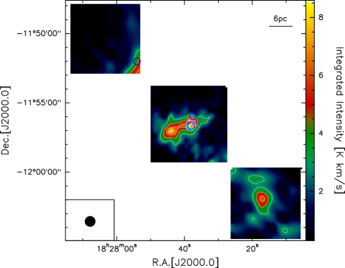
Figure 12: FCRAO intensity map of the C¹⁸O(1-0) emission, integrated between 25 and 57 km s^-1. The contour levels are from 10 $\sigma$ in steps of 5 $\sigma$ ($\sigma$= 0.3 K km s^-1). Symbols are as in Fig. 1 (see Table 9).

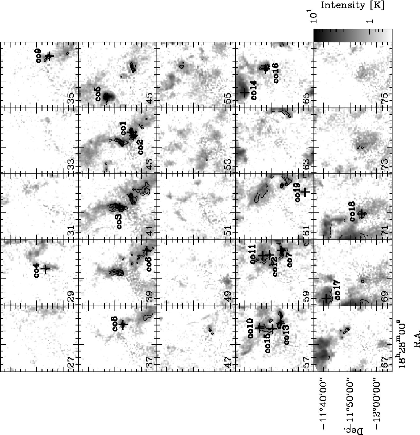
Figure 13: Channel map of the BU-FCRAO GRS ¹³CO(1-0) data in grey scale and our FCRAO ¹³CO(1-0) emission in black contours. Center velocities of the channels are indicated in the bottom left corner of each panel and increase in steps of 2 km s^-1. Contour levels are drawn from 10 $\sigma$ ($\sigma$ = 0.2 K) in steps of 5 $\sigma$. The black numbered crosses indicate the peak positions (in the channel corresponding to the peak velocity) of the emission of the 19 molecular clumps identified in the FCRAO ¹³CO(1-0) emission.

FCRAO ¹³CO(1-0)                                            APEX 870 $\mu$m

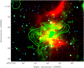
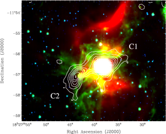
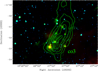
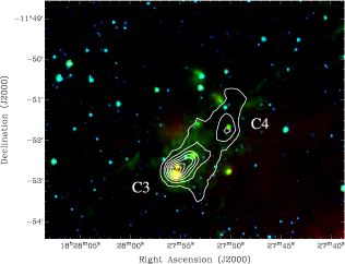
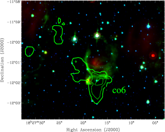
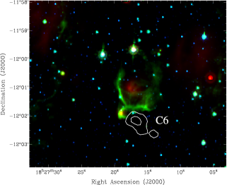
Figure 14: Composite image of the 24 $\mu$m (red), the 8 $\mu$m (green) and 3.6 $\mu$m (blue) emissions from Spitzer, covering several regions of the large-scale map, corresponding to the single clumps associated with the APEX continuum emission at 870 $\mu$m. The green contours are the ¹³CO(1-0) emission of the single clumps, integrated over the velocity range of every clump (see col. 4 of Table 3), and the white contours are the APEX continuum emission at 870 $\mu$m (from 5 $\sigma$ in steps of 5 $\sigma$, where $\sigma=40$ mJy beam^-1). The ¹³CO clumps and the correspondent continuum sources are labelled in the single diagrams. Note that some of the panels are similar because for each clump we integrated on the velocity channels of emission of the clump (see col. 4 of Table 3).

FCRAO ¹³CO(1-0)                                            APEX 870 $\mu$m

Fig. 14 – Continued.

FCRAO ¹³CO(1-0)                            APEX 870 $\mu$m                  

Fig. 14 – Continued.