Magnetic helicity flux in the presence of shear

Abstract

Magnetic helicity has risen to be a major player in dynamo theory, with the helicity of the small-scale field being linked to the dynamo saturation process for the large-scale field. It is a nearly conserved quantity, which allows its evolution equation to be written in terms of production and flux terms. The flux term can be decomposed in a variety of fashions. One particular contribution that has been expected to play a significant role in dynamos in the presence of mean shear was isolated by Vishniac & Cho (2001, ApJ 550, 752). Magnetic helicity fluxes are explicitly gauge dependent however, and the correlations that have come to be called the Vishniac–Cho flux were determined in the Coulomb gauge, which turns out to be fraught with complications in shearing systems. While the fluxes of small-scale helicity are explicitly gauge dependent, their divergences can be gauge independent. We use this property to investigate magnetic helicity fluxes of small-scale field through direct numerical simulations in a shearing-box system and find that in a numerically usable gauge the divergence of the small-scale helicity flux vanishes, while the divergence of the Vishniac–Cho flux remains finite. We attribute this seeming contradiction to the existence of horizontal fluxes of small-scale magnetic helicity with finite divergences.

1. Introduction

The large-scale magnetic field of the Sun and other stars is often modeled using mean-field theory (Rüdiger & Hollerbach, 2004). Important ingredients in this theory are the $\alpha$ effect responsible for field amplification and an enhanced (turbulent) magnetic diffusivity Moffatt (1978); Krause & Rädler (1980). Once the field has reached appreciable field strength, these effects become modified through the backreaction of the Lorentz force. Often a simple algebraic quenching formula is being assumed, but such a simple prescription is unable to model correctly the quenching under more general conditions with shear (Brandenburg et al., 2001) or boundaries (Brandenburg & Dobler, 2001).

Over the past decade, significant progress has been made in modeling the dynamo saturation process in mean-field models through the development and use of the dynamical $\alpha$ quenching methodology. This methodology (originally due to Kleeorin & Ruzmaikin, 1982) has explained several puzzling features of MHD dynamos, such as the slow saturation phase of a homogeneous $\alpha^{2}$ dynamo (Field & Blackman, 2002; Blackman & Brandenburg, 2002), and has reposed the crucial question of catastrophic $\alpha$ quenching (see Brandenburg & Subramanian, 2005a, for a review). In this picture, the saturation of the dynamo is caused by the build-up of magnetic helicity, which is nearly conserved in the high conductivity limit in the absence of fluxes. This raises the possibility of speeding up the saturation process and reaching significant saturation field strength through mechanisms that export or destroy magnetic helicity.

Making general use of the dynamical $\alpha$ quenching methodology in open systems then requires an understanding of magnetic helicity fluxes, more significantly an understanding of the fluxes of magnetic helicity of the small-scale field. In the following we often refer to such fluxes as small-scale magnetic helicity fluxes, although this is not quite accurate, because it is itself a mean quantity and not a fluctuation. Recent work has shown that in inhomogeneous systems there is a turbulent diffusive flux of small-scale helicity, at least in the absence of shear, although the diffusion coefficient is in some cases smaller than expected (Mitra et al., 2010; Hubbard & Brandenburg, 2010). Consideration of that flux term has allowed mean-field models to capture the saturation behavior of some non-triply periodic, non-homogeneous dynamos without shear. Unfortunately, the fluxes of small-scale magnetic helicity are explicitly gauge dependent, and in the presence of turbulence, can be decomposed in different fashions.

In Vishniac & Cho (2001), an interesting component of the flux of small-scale helicity was isolated. This component has been named the Vishniac–Cho flux, henceforth the VC flux. In later work (Subramanian & Brandenburg, 2004; Brandenburg & Subramanian, 2005b), the form of this flux in the presence of uniform shear was calculated, and found to be both simple and of significant magnitude. Shear drives an $\Omega$ effect and is an important and nearly omni-present player in astrophysical dynamos, so the VC flux has seen significant interest, both in mean-field modeling (Brandenburg & Subramanian, 2005b) and in the interpretation of the differences between similar direct numerical simulations with differing boundary conditions (Brandenburg, 2005; Käpylä et al., 2008). It is important to realize however that shear poses unique difficulties in the formulation, and importantly, interpretation, of magnetic helicity fluxes. It is the goal of this paper to explore those difficulties and determine the significance of the VC flux. We use the perhaps surprising result that while magnetic helicity fluxes are gauge dependent, their divergences may not be across broad gauge-families (Mitra et al., 2010) to allow us to compare the VC flux with the small-scale magnetic helicity flux in a gauge where the mean shear is easy to treat. Our investigations will bear weight on the interpretation and use of the VC flux, but we will not and indeed cannot extract the VC flux from the simulations we perform.

In Section 2 we discuss the various contributions to the magnetic helicity flux and define our mean-field decomposition. Further, we explain the broad gauge independence of small-scale magnetic helicity flux divergences. In Section 3 we sketch the difficulties inherent in uniform shear, define the shearing-advective gauge and derive the small-scale magnetic helicity flux in that gauge. In Section 4 we discuss the VC flux as calculated in Subramanian & Brandenburg (2004) and Brandenburg & Subramanian (2005b). In Section 5 we present the results of our direct numerical simulations and compare the results with the VC flux. We discuss the significance of our results in Section 6 and conclude in Section 7.

2. Magnetic helicity flux and formalism

We begin by deriving the formula for magnetic helicity fluxes in general. The MHD equations for the magnetic field are:

$$\mbox{\boldmath$B$}{}=\mbox{\boldmath$\nabla$}{}\times\mbox{\boldmath$A$}{},$$ (1)

$$\mbox{\boldmath$J$}{}=\mbox{\boldmath$\nabla$}{}\times\mbox{\boldmath$B$}{}/\mu_{0},$$ (2)

$$\mbox{\boldmath$E$}{}=-\mbox{\boldmath$U$}{}\times\mbox{\boldmath$B$}{}+\eta\mu_{0}\mbox{\boldmath$J$}{},$$ (3)

$$\frac{\partial\mbox{\boldmath$A$}{}}{\partial t}=-\mbox{\boldmath$E$}{}-\mbox{\boldmath$\nabla$}{}\Phi,$$ (4)

where $\eta$ is the molecular resistivity, $\mu_{0}$ is the vacuum permeability, and $\Phi$ is the electrostatic or scalar potential that determines our gauge. For example, setting $\Phi=0$ results in the Weyl gauge, of interest numerically because it simplifies Equation (4), while a solution of Equation (4) with $\mbox{\boldmath$\nabla$}{}^{2}\Phi=-\mbox{\boldmath$\nabla$}{}\cdot\mbox{\boldmath$E$}{}$ will have constant $\mbox{\boldmath$\nabla$}{}\cdot\mbox{\boldmath$A$}{}$ and with an appropriate initial condition on $A$ results in the Coulomb gauge.

The time evolution of the magnetic helicity density $h\equiv\mbox{\boldmath$A$}{}\cdot\mbox{\boldmath$B$}{}$ is then given by

$$\frac{\partial h}{\partial t} = \frac{\partial\mbox{\boldmath$A$}{}}{\partial t}\cdot\mbox{\boldmath$B$}{}+\mbox{\boldmath$A$}{}\cdot\frac{\partial\mbox{\boldmath$B$}{}}{\partial t}$$ (5)

$$= -2\eta\mu_{0}\mbox{\boldmath$J$}{}\cdot\mbox{\boldmath$B$}{}-\mbox{\boldmath$\nabla$}{}\cdot\left(\mbox{\boldmath$E$}{}\times\mbox{\boldmath$A$}{}+\Phi\mbox{\boldmath$B$}{}\right).$$

The flux $\mbox{\boldmath$F$}{}_{\Phi}$ of magnetic helicity in a given gauge with a corresponding $\Phi$ can be read out of Equation (5):

$$\mbox{\boldmath$F$}{}_{\Phi} = \mbox{\boldmath$E$}{}\times\mbox{\boldmath$A$}{}+\Phi\mbox{\boldmath$B$}{}=-\left(\mbox{\boldmath$U$}{}\times\mbox{\boldmath$B$}{}\right)\times\mbox{\boldmath$A$}{}+\Phi\mbox{\boldmath$B$}{}+\eta\mu_{0}\mbox{\boldmath$J$}{}\times\mbox{\boldmath$A$}{}$$ (6)

$$= h\mbox{\boldmath$U$}{}+(\Phi-\mbox{\boldmath$U$}{}\cdot\mbox{\boldmath$A$}{})\mbox{\boldmath$B$}{}+\eta\mu_{0}\mbox{\boldmath$J$}{}\times\mbox{\boldmath$A$}{}.$$

In Equation (6) we recognize the advective flux $\mbox{\boldmath$F$}{}_{\text{adv}}\equiv h\mbox{\boldmath$U$}{}$, a resistive flux $\mbox{\boldmath$F$}{}_{\text{res}}\equiv\eta\mu_{0}\mbox{\boldmath$J$}{}\times\mbox{\boldmath$A$}{}$, and finally a dynamical flux,

$$\mbox{\boldmath$F$}{}_{\text{dyn}}\equiv(\Phi-\mbox{\boldmath$U$}{}\cdot\mbox{\boldmath$A$}{})\mbox{\boldmath$B$}{}.$$ (7)

The formula for $\mbox{\boldmath$F$}{}_{\text{dyn}}$ leads us to consider “advective” gauges of the form $\Phi\equiv\mbox{\boldmath$U$}{}^{\prime}\cdot\mbox{\boldmath$A$}{}$, where $\mbox{\boldmath$U$}{}^{\prime}$ is one component of the velocity field, see Section 3.1.

2.1. Mean-field decomposition

We proceed to a mean-field decomposition of the magnetic helicity flux. We denote general averaging schemes by overbars. Fluctuating terms will be denoted by lower cases or primes:

$$\mbox{\boldmath$A$}{}=\overline{\mbox{\boldmath$A$}{}}+\mbox{\boldmath$a$}{},\quad\mbox{\boldmath$A$}{}\cdot\mbox{\boldmath$B$}{}=\overline{\mbox{\boldmath$A$}{}\cdot\mbox{\boldmath$B$}{}}+\left(\mbox{\boldmath$A$}{}\cdot\mbox{\boldmath$B$}{}\right)^{\prime}.$$ (8)

The mean-field decomposition of Equations (4) and (5) yields

$$\frac{\partial\overline{\mbox{\boldmath$A$}{}}}{\partial t}=\overline{\mbox{\boldmath$U$}{}}\times\overline{\mbox{\boldmath$B$}{}}+\overline{\mbox{\boldmath${\cal E}$}{}}-\eta\mu_{0}\overline{\mbox{\boldmath$J$}{}}-\mbox{\boldmath$\nabla$}{}\overline{\Phi},$$ (9)

where $\overline{\mbox{\boldmath${\cal E}$}{}}\equiv\overline{\mbox{\boldmath$u$}{}\times\bm{b}}$ and

$$\frac{\partial\overline{h}}{\partial t}=-2\eta\mu_{0}\overline{\mbox{\boldmath$J$}{}\cdot\mbox{\boldmath$B$}{}}-\mbox{\boldmath$\nabla$}{}\cdot\overline{\mbox{\boldmath$E$}{}\times\mbox{\boldmath$A$}{}}-\mbox{\boldmath$\nabla$}{}\cdot\overline{\Phi\mbox{\boldmath$B$}{}}.$$ (10)

The latter can be written as

$$\frac{\partial\overline{h}}{\partial t}=\frac{\partial\overline{h}_{\text{m}}}{\partial t}+\frac{\partial\overline{h}_{\text{f}}}{\partial t},$$ (11)

where $\overline{h}=\overline{h}_{\text{m}}+\overline{h}_{\text{f}}$, with $\overline{h}_{\text{m}}\equiv\overline{\mbox{\boldmath$A$}{}}\cdot\overline{\mbox{\boldmath$B$}{}}$ being the helicity in the large-scale fields and $\overline{h}_{\text{f}}\equiv\overline{\mbox{\boldmath$a$}{}\cdot\bm{b}}$ the helicity in the small-scale fields.

The evolution equations for these helicities are

$$\frac{\partial\overline{h}_{\text{m}}}{\partial t}= + 2\overline{\mbox{\boldmath${\cal E}$}{}}\cdot\overline{\mbox{\boldmath$B$}{}}-2\eta\mu_{0}\overline{\mbox{\boldmath$J$}{}}\cdot\overline{\mbox{\boldmath$B$}{}}-\mbox{\boldmath$\nabla$}{}\cdot\left(\overline{\mbox{\boldmath$E$}{}}\times\overline{\mbox{\boldmath$A$}{}}+\overline{\Phi}\overline{\mbox{\boldmath$B$}{}}\right),$$ (12)

$$\frac{\partial\overline{h}_{\text{f}}}{\partial t}= - 2\overline{\mbox{\boldmath${\cal E}$}{}}\cdot\overline{\mbox{\boldmath$B$}{}}-2\eta\mu_{0}\overline{\mbox{\boldmath$j$}{}\cdot\bm{b}}-\mbox{\boldmath$\nabla$}{}\cdot\left(\overline{\mbox{\boldmath$e$}{}\times\mbox{\boldmath$a$}{}}+\overline{\phi\bm{b}}\right),$$ (13)

where $\phi=\Phi-\overline{\Phi}$ is the fluctuating scalar potential and

$$\overline{\mbox{\boldmath${\cal E}$}{}}=\alpha\overline{\mbox{\boldmath$B$}{}}-\eta_{\rm t}\mu_{0}\overline{\mbox{\boldmath$J$}{}}$$ (14)

is the mean turbulent electromotive force, where $\alpha$ is the $\alpha$ effect and $\eta_{\rm t}$ is the turbulent magnetic diffusivity. From Equations (12) and (13) we find the fluxes of the large-scale and small-scale fields:

$$\overline{\bm{F}}_{\text{m}} = \overline{\mbox{\boldmath$E$}{}}\times\overline{\mbox{\boldmath$A$}{}}+\overline{\Phi}\overline{\mbox{\boldmath$B$}{}},$$ (15)

$$\overline{\bm{F}}_{\text{f}} = \overline{\mbox{\boldmath$e$}{}\times\mbox{\boldmath$a$}{}}+\overline{\phi\bm{b}}.$$ (16)

2.2. The significance of gauges for magnetic helicity fluxes

It is clear from the form of $\mbox{\boldmath$F$}{}_{\text{dyn}}$ in Equation (7) that any consideration of helicity fluxes must also take into account the gauge choice, as at any point where $\mbox{\boldmath$F$}{}_{\text{dyn}}\neq 0$, the value of $\mbox{\boldmath$F$}{}_{\text{dyn}}$ can be arbitrarily set by the gauge or, equivalently, the condition for $\mbox{\boldmath$F$}{}_{\text{dyn}}$ being independent of $\Phi$ is that $\mbox{\boldmath$F$}{}_{\text{dyn}}=0$ for all gauges. A gauge choice that generates a desired flux along $\bm{\hat{x}}$ is always possible provided $\mbox{\boldmath$B$}{}\cdot\hat{\bm{x}}\neq 0$. Such a gauge takes the form $\Phi(\bm{x},t)=f(\bm{x},t)B_{x}$. Recall also that boundary or symmetry conditions on the physical system do not apply to the vector potential or the gauge (although numerical simulations may require gauge choices where they do). The ability to add an arbitrary flux of magnetic helicity to the system via the addition of a new gauge makes the isolation of differing components of the flux a risky business.

There are effects that mitigate this gauge dependence however. The divergence of $\mbox{\boldmath$F$}{}_{\text{f}}$ and the term $\partial\overline{h}/\partial t$ are the only gauge-dependent terms in Equation (13). If $\overline{h}_{\text{f}}$ is indeed gauge independent then the divergence of $\mbox{\boldmath$F$}{}_{\text{f}}$ must be gauge independent as well, even though the flux itself is explicit gauge dependent. Clearly the divergence of $\mbox{\boldmath$F$}{}_{\text{f}}$ is the same for all gauges for which $\partial_{t}\overline{h}_{\text{f}}$ is the same. As long as our shearing-box has a time-constant $\overline{h}_{\text{f}}$ in the saturated regime, we can make statements about the divergence of $\mbox{\boldmath$F$}{}_{\text{f}}$ for all gauges which would have a time-constant saturated $\overline{h}_{\text{f}}$.

The dynamical $\alpha$ quenching methodology, one of the primary consumers of magnetic helicity information, assumes that the small-scale magnetic helicity $\overline{h}_{\text{f}}$ and the small-scale current helicity $\overline{\mbox{\boldmath$j$}{}\cdot\bm{b}}$ are proportional. This requirement is often used as an argument in favor of the Coulomb gauge (Kleeorin & Rogachevskii, 1999). Even if the saturated current helicity is not time-independent (as might be the case for an oscillating solution), as the current helicity is gauge independent, the validity of the dynamic $\alpha$ quenching methodology assumes therefore that the former is as well. Recent studies have supported this hypothesis (Mitra et al., 2010; Hubbard & Brandenburg, 2010), at least in the limits of numerical simulations, which disallow extreme levels of gauge pathology by forcing the vector potential to be numerically resolved. (This will be discussed in more detail in a separate paper where we solve an evolution equation for the gauge transformation.) Alternatively, one could restrict oneself to families of gauges where the relation holds. We note that, in that regard, both the magnetic and current helicities are shearing-periodic in our system in the shearing-advective gauge that will be described later, while in the Weyl gauge the magnetic helicity is not .

3. Shear

The presence of shear poses further difficulties when considering magnetic helicity fluxes. To see this, consider a shearing periodic box with an imposed flow, $\mbox{\boldmath$U$}{}_{S}=(0,Sx,0)$, and sides of length $L$ centered on the origin. We will use the Weyl gauge ($\Phi=0)$ and a planar averaging scheme:

$$\overline{\mbox{\boldmath$B$}{}}(x,y,z,t)\equiv L^{-2}\int_{-L/2}^{L/2}\int_{-L/2}^{L/2}dx^{\prime}dy^{\prime}\mbox{\boldmath$B$}{}(x^{\prime},y^{\prime},z,t).$$ (17)

In what follows, we will assume that the shear flow is the only large-scale velocity, and note that it averages to $0$ and so technically is a fluctuating field. This could in principle be avoided under a local planar average over a square centered on $(x,y)$ for example (Brandenburg et al., 2008). However, such an average is problematic too, because it does not obey one of the Reynolds rules: the average of a product of an average and a fluctuation does not vanish. Nevertheless, even though uniform shear can complicate averaging schemes, it is easier to treat than non-uniform shear with the resulting non-uniform $\Omega$ effect. We therefore proceed with our standard (non-sliding) averaging scheme. We will also assume that, at the single instant in time that we consider, the vector potential $A$ is shearing periodic as well. Note that in the Weyl gauge, the vector potential will not remain shearing periodic. Numerical simulations in the shearing box approximation use therefore a different gauge (Brandenburg et al., 1995), as will be discussed below.

The difficulty in treating the helicity flux can be seen from Equation (6) which, in the Weyl gauge, becomes

$$\mbox{\boldmath$F$}{}=h\mbox{\boldmath$U$}{}_{S}-(\mbox{\boldmath$U$}{}_{S}\cdot\mbox{\boldmath$A$}{})\mbox{\boldmath$B$}{}+h\mbox{\boldmath$u$}{}-(\mbox{\boldmath$u$}{}\cdot\mbox{\boldmath$A$}{})\mbox{\boldmath$B$}{}+\eta\mu_{0}\mbox{\boldmath$J$}{}\times\mbox{\boldmath$A$}{}.$$ (18)

If $A$ were shearing periodic, the last four terms of Equation (18) would be likewise shearing periodic and hence would not contribute a net divergence to the system. However, the first two terms on the right-hand side of Equation (18) violate shearing-periodicity. In particular, the $x$ component of the second term on the right-hand side of Equation (18) reduces to

$$F_{x}=-(\mbox{\boldmath$U$}{}_{S}\cdot\mbox{\boldmath$A$}{})B_{x}+...=-SxA_{y}B_{x}+...,$$ (19)

where the dropped terms cannot contribute a net divergence. Recall that, at first, $A_{y}B_{x}$ would here still be shearing periodic. Systems with shearing-periodic magnetic vector potentials would then allow for a horizontal flux of magnetic helicity.

3.1. Helicity fluxes in advective gauges

To examine the VC flux numerically, we adopt a homogeneous shearing-periodic setup. (The resulting magnetic field will however become inhomogeneous and could produce finite magnetic helicity fluxes and flux divergences.) As discussed above, to keep the magnetic vector potential itself shearing-periodic we must use an appropriate gauge, namely $\Phi=\mbox{\boldmath$U$}{}_{S}\cdot\mbox{\boldmath$A$}{}$, which we term “shearing-advective”. This is also the gauge used by Brandenburg et al. (1995). More generally, we can define a family of “advective gauges” with $\Phi_{A}=\mbox{\boldmath$U$}{}_{A}\cdot\mbox{\boldmath$A$}{}$, for a component of the velocity $\mbox{\boldmath$U$}{}_{A}$, with the corresponding $\mbox{\boldmath$U$}{}_{NA}=\mbox{\boldmath$U$}{}-\mbox{\boldmath$U$}{}_{A}$. The name “advective” is chosen because in this gauge the effect of $\mbox{\boldmath$U$}{}_{A}$ on the helicity flux is advective as can be seen from Equation (6), which becomes:

$$\mbox{\boldmath$E$}{}_{A} = -\mbox{\boldmath$U$}{}_{NA}\times\mbox{\boldmath$B$}{}+\eta\mu_{0}\mbox{\boldmath$J$}{},$$ (20)

$$\mbox{\boldmath$F$}{}_{\Phi} = h\mbox{\boldmath$U$}{}_{A}+(\mbox{\boldmath$E$}{}_{A}\times\mbox{\boldmath$A$}{}).$$ (21)

If $\mbox{\boldmath$U$}{}_{A}$ is a mean flow ($\overline{\mbox{\boldmath$U$}{}}_{A}=\mbox{\boldmath$U$}{}_{A}$), then the mean flux of the small-scale helicity becomes

$$\overline{\bm{F}}_{\text{f}}=\overline{h}_{\text{f}}\overline{\mbox{\boldmath$U$}{}}_{A}+\overline{\mbox{\boldmath$e$}{}_{A}\times\mbox{\boldmath$a$}{}}.$$ (22)

Alternatively, if $\mbox{\boldmath$U$}{}_{A}$ is not a mean flow ($\overline{\mbox{\boldmath$U$}{}}_{A}=0$), then we have

$$\overline{\bm{F}}_{\text{f}}=\overline{h_{\rm f}^{\prime}\mbox{\boldmath$U$}{}_{A}^{\prime}}+\overline{\mbox{\boldmath$e$}{}_{A}\times\mbox{\boldmath$a$}{}}.$$ (23)

For our system, with $\mbox{\boldmath$U$}{}_{A}=\mbox{\boldmath$U$}{}_{S}$, $\mbox{\boldmath$e$}{}_{A}$, $a$ and $\bm{b}$ are all shearing-periodic, and so their mean values, as well as all other mean values, are functions of $z$ alone. Correspondingly, only the $z$ component of $\mbox{\boldmath$F$}{}_{\text{f}}$ can have a finite divergence, and we have eliminated the worry of horizontal magnetic helicity fluxes. Further, to the extent that the system is homogeneous, and invariant under a $180$ degree rotation about the $z$ axis, the horizontal fluxes vanish entirely except for the advective flux due to the shear flow.

4. The Vishniac–Cho flux with mean shear

The VC flux, $\overline{\bm{F}}_{\text{VC}}$, has been calculated in several places using the first order smoothing approximation and later the $\tau$ approximation. Their applicability to highly turbulent systems with large magnetic Reynolds numbers cannot be guaranteed and is subject to verification by numerical simulations, although it should work in cases of small magnetic Reynolds numbers considered in this paper. This flux was originally calculated in the Coulomb gauge, but it can be calculated in a related gauge in which the magnetic helicity density corresponds to a density of magnetic linkages (Subramanian & Brandenburg, 2006). It is most interesting in the case of shear, and we will restrict ourselves to the consideration of uniform shear which, as noted above, raises concerns about horizontal fluxes with finite divergence. In this system, $\overline{\bm{F}}_{\text{VC}}$ was calculated in the appendix of Brandenburg & Subramanian (2005b) to be

$$\overline{\bm{F}}_{\text{VC}}=C_{\text{VC}}\,{S\hat{\bm{z}}\over 2k_{\rm f}^{2}}\,(\overline{B}_{x}^{2}-\overline{B}_{y}^{2}),$$ (24)

where $C_{\text{VC}}$ is a coefficient expected to be of order unity and $k_{\rm f}$ is the wavenumber of the energy-carrying eddies. As eluded to in Section 2.2, we assume here that the current helicity is proportional to $k_{\rm f}^{2}$ times the magnetic helicity density. There are other components of the magnetic helicity flux known, for example the term in Equation (19) can be found in the $\mbox{\boldmath$F$}{}^{\rm bulk}$ of Subramanian & Brandenburg (2006), and, as noted in Section 2.2, the interesting value is the divergence of the total of all fluxes, which might pick up contributions from the $x$ component of the flux.

While the VC flux is of pressing interest to mean-field dynamo theory and it has been invoked in the interpretation of numerical simulations (Käpylä et al., 2008), the work on its implications in mean-field theory is not well developed. In Section 5.2 we present a brief mean-field analysis of the effects of a VC flux in our shearing-sheet system using (24), and compare those results to the work of Guerrero et al. (2010) in spherical shells.

5. Model calculations

5.1. Preliminary considerations

In order to quantify shear-driven magnetic helicity fluxes, we consider the shearing box approximation (Wisdom & Tremaine, 1988) with periodic boundary conditions in the $y$ and $z$ directions and shearing-periodic boundary conditions in the $x$ direction. According to Equation (24) we expect a magnetic helicity flux in the $z$ direction. However, because our system is periodic in the $z$ direction, there will be no net magnetic helicity flux in or out of the domain. Nevertheless, the local divergence of $\overline{\bm{F}}_{\text{VC}}$ should be finite because, contrary to homogeneous $\alpha^{2}$ dynamos without shear, $\overline{B}_{x}^{2}-\overline{B}_{y}^{2}$ is in general $z$-dependent for $\alpha\Omega$ dynamos. Indeed, the mean field that develops is a reasonable approximation to an $\alpha\Omega$ dynamo, where $|S|>|\alpha k_{z}|$. The marginally excited kinematic solution of a mean-field $\alpha\Omega$ dynamo is a traveling wave (see, e.g., Brandenburg & Sokoloff, 2002), i.e.

$$\overline{\mbox{\boldmath$B$}{}}=B_{0}\left(\sin\theta,\sqrt{2}\left|\frac{c}{\alpha}\right|\sin(\theta+\chi),0\right)$$ (25)

with

$$c=\pm\left|\frac{\alpha S}{2k_{z}}\right|^{1/2}\!\!=\pm\eta_{T}k_{z},\quad\theta=k_{z}(z-ct),\quad\chi=\mp{3\over 4}\pi,$$ (26)

where the sign in front of $c$ is given by the sign of the product $\alpha S$ and $B_{0}$ is an undetermined amplitude factor. Note that the magnetic helicity of this large-scale field, $\overline{h}_{\text{m}}=|c/\alpha|k_{z}^{-1}B_{0}^{2}$, is independent of $z$ for the “natural” vector potential

$$\overline{\mbox{\boldmath$A$}{}}=k_{z}^{-1}B_{0}\left(-\sqrt{2}\left|\frac{c}{\alpha}\right|\cos(\theta+\chi),\cos\theta,0\right).$$ (27)

The point of this discussion is to emphasize that even for an initially homogeneous system, Equation (4) would predict the appearance of a magnetic helicity flux. This flux would lead to the annihilation of magnetic helicity fluctuations of opposite sign — even if such fluctuations were not present initially. The effect of such fluxes can be predicted by mean-field models with catastrophic quenching included (Brandenburg et al., 2009). As we will show in the next section, the VC flux has actually an adverse effect on the saturation behavior, and that only fluxes with the opposite sign are able to accelerate the saturation of the mean field.

5.2. Mean-field model with diffusive and VC fluxes

To demonstrate the difference between mean-field predictions with and without the presence of a VC flux that is not compensated for by other fluxes we use a mean-field dynamical $\alpha$ quenching model (Kleeorin & Ruzmaikin, 1982; Blackman & Brandenburg, 2002; Brandenburg et al., 2009). This methodology combines the dynamical $\alpha$ quenching equations

$$\alpha(z,t)=\alpha_{K}+\alpha_{M},\quad\alpha_{M}=\eta_{\rm t}k_{\rm f}^{2}\frac{\overline{h}_{\text{f}}}{B_{\rm eq}^{2}},$$ (28)

$$\frac{\partial\alpha_{M}}{\partial t}=-2\eta_{\rm t}k_{\rm f}^{2}\left(\frac{\overline{\mbox{\boldmath${\cal E}$}{}}\cdot\overline{\mbox{\boldmath$B$}{}}}{B_{\rm eq}^{2}}+\frac{\alpha_{M}}{\mbox{\rm Re}_{M}}\right)-\mbox{\boldmath$\nabla$}{}\cdot\overline{\mbox{\boldmath$F$}{}}_{\alpha},$$ (29)

with the standard mean-field equation (in the shearing-advective gauge with $\overline{\mbox{\boldmath$U$}{}}=0$):

$$\frac{\partial\overline{\mbox{\boldmath$A$}{}}}{\partial t}=-S\overline{A}_{y}\hat{\mbox{\boldmath$x$}}{}+\overline{\mbox{\boldmath${\cal E}$}{}}-\eta\mu_{0}\overline{\mbox{\boldmath$J$}{}},$$ (30)

where the $\overline{\mbox{\boldmath${\cal E}$}{}}$ is given by Equation (14).

We test diffusive and VC fluxes, setting

$$\overline{\mbox{\boldmath$F$}{}}_{\alpha}=\frac{\eta_{\rm t}k_{\rm f}^{2}}{B_{\rm eq}^{2}}\left(\overline{\bm{F}}_{\text{VC}}-\kappa_{\alpha}\mbox{\boldmath$\nabla$}{}\overline{h}_{\text{f}}\right).$$ (31)

We measure the strength of the kinetic $\alpha$ effect $\alpha_{K}$ and the shear $S$ with the dynamo numbers

$$C_{\alpha}\equiv\frac{\alpha_{K}}{\eta_{\rm t}k_{1}}\simeq\frac{k_{\rm f}}{k_{1}},\quad C_{S}\equiv\frac{S}{\eta_{\rm t}k_{1}^{2}},$$ (32)

where $k_{1}=2\pi/L_{z}$ is the minimal wavenumber of the domain in the $z$ direction. Note that $\alpha_{K}$ is assumed independent of $\overline{\mbox{\boldmath$B$}}{}$, so the kinetic $\alpha$ effect is therefore also a kinematic one.

The results are shown in Figure 1, where we plot the saturation behavior of models with $\eta_{\rm t}/\eta=10^{3}$, and dynamo numbers $C_{\alpha}=-0.2$ and $C_{S}=-20$. The left panel covers four values of $\kappa_{\alpha}/\eta_{\rm t}$ the turbulent diffusion coefficient for $\overline{h}_{\text{f}}$, with the VC flux turned off ($C_{\text{VC}}=0$). The right panel displays the dynamo behavior for three values of $C_{\rm VC}$ with $\kappa_{\alpha}/\eta_{\rm t}=0.2$. Note that in all calculations an early intermediate saturation level of $\approx 0.15B_{\rm eq}$ is reached. This is followed by a resistively slow saturation phase, as was expected from models without shear (Brandenburg, 2001; Blackman & Brandenburg, 2002). In agreement with earlier work, the saturation behavior is accelerated by diffusive fluxes (Brandenburg et al., 2009). In the absence of a diffusive flux, $\kappa_{\alpha}=0$, the field drops suddenly back to lower values and continues to oscillate. These oscillations are eliminated by small values of $\kappa_{\alpha}$ while not significantly affecting the intermediate saturation behavior if $\kappa_{\alpha}=0.2\eta_{\rm t}$. Note that for positive values of $C_{\text{VC}}$, the VC flux actually has an adverse effect on the saturation behavior and only negative values are able to accelerate the saturation. This is similar to results for mean-field dynamo action in spherical shells (Guerrero et al., 2010).

Figure 1.— Left: Saturation behavior of models with $\eta_{\rm t}/\eta=10^{3}$, $C_{\text{VC}}=0$, $C_{\alpha}=-0.2$, and $C_{S}=-20$, and for $\kappa_{\alpha}/\eta_{\rm t}$ ranging from 0 to 1. Right: Same, but for $C_{\rm VC}$ ranging from $-0.2$ to $+0.2$ and $\kappa_{\alpha}/\eta_{\rm t}=0.2$.

5.3. Simulations of shear flow turbulence

We turn to the computation of magnetic helicity fluxes through direct numerical simulations. We solve the stochastically forced isothermal hydromagnetic equations in a generally cubical domain of size $(2\pi)^{3}$ in the presence of a uniform shear flow, $\mbox{\boldmath$U$}{}_{S}=(0,Sx,0)$, with $S={\rm const}{}$,

$${{\cal D}{}\mbox{\boldmath$A$}{}\over{\cal D}{}t}=-SA_{y}\hat{\mbox{\boldmath$x$}}{}+\mbox{\boldmath$U$}{}\times\mbox{\boldmath$B$}{}+\eta\nabla^{2}\mbox{\boldmath$A$}{},$$ (33)

$${{\cal D}{}\mbox{\boldmath$U$}{}\over{\cal D}{}t}=-SU_{x}\hat{\mbox{\boldmath$y$}}{}-c_{\rm s}^{2}\mbox{\boldmath$\nabla$}{}\ln\rho+{1\over\rho}\mbox{\boldmath$J$}{}\times\mbox{\boldmath$B$}{}+\mbox{\boldmath$F$}{}_{\rm visc}+\mbox{\boldmath$f$}{},$$ (34)

$${{\cal D}{}\ln\rho\over{\cal D}{}t}=-\mbox{\boldmath$\nabla$}{}\cdot\mbox{\boldmath$U$}{},$$ (35)

where ${\cal D}{}/{\cal D}{}t=\partial/\partial t+(\mbox{\boldmath$U$}{}+\mbox{\boldmath$U$}{}_{S})\cdot\mbox{\boldmath$\nabla$}{}$ is the advective derivative with respect to the total flow velocity that also includes the shear flow, $c_{\rm s}={\rm const}{}$ is the isothermal sound speed, $\mbox{\boldmath$F$}{}_{\rm visc}=\rho^{-1}\mbox{\boldmath$\nabla$}{}\cdot(2\rho\nu\mbox{\boldmath${\sf S}$}{})$ is the viscous force, ${\mathsf{S}}_{ij}={\textstyle{1\over 2}}(U_{i,j}+U_{j,i})-{\textstyle{1\over 3}}\delta_{ij}\mbox{\boldmath$\nabla$}{}\cdot\mbox{\boldmath$U$}{}$ is the traceless rate-of-strain tensor, commas denote partial differentiation, and $f$ is the forcing term. As in earlier work (Brandenburg, 2001) the forcing function consists of plane polarized waves whose direction and phase change randomly from one time step to the next. The modulus of its wavevectors is taken from a band of wavenumbers around a given average wavenumber that is referred to as $k_{\rm f}$.

The main control parameters in our simulations are the magnetic Reynolds and Prandtl numbers, as well as the shear parameter,

$$\mbox{\rm Re}_{M}={u_{\rm rms}\over\eta k_{\rm f}},\quad\mbox{\rm Pr}_{M}={\nu\over\eta},\quad\mbox{\rm Sh}={S\over u_{\rm rms}k_{\rm f}}.$$ (36)

We adopt periodic boundary conditions in the $y$ and $z$ directions and shearing-periodic boundary conditions in the $x$ direction. Our initial velocity, in addition to $\mbox{\boldmath$U$}{}_{S}$, is $\mbox{\boldmath$U$}{}=\bm{0}$ and the initial density is $\rho=\rho_{0}\equiv{\rm const}{}$, while for the magnetic field we take a Beltrami field of negative magnetic helicity and low amplitude ($10^{-7}$ times the equipartition value). The magnetic field grows then exponentially owing to dynamo action and saturates when the field reaches a certain multiple of the equipartition value. We solve the governing equations using the Pencil Code which is a high-order finite-difference code (sixth order in space and third order in time) for solving partial differential equations on massively parallel machines. Our model setup is identical to that used by Käpylä & Brandenburg (2009), who studied the frequency of dynamo waves in the saturated regime as a function of the fractional helicity and thereby the effective dynamo number and, more importantly, different magnetic field strengths.

5.4. The VC flux in simulations

We focus here on the results of four simulations, with parameters given in Table LABEL:pars. Standard estimates suggest that the two dynamo parameters given in Equation (32) suffice for large-scale dynamo action ($C_{\alpha}C_{S}>2$), and also their ratio, $C_{S}/C_{\alpha}\approx 3\mbox{\rm Sh}\ k_{\rm f}/k_{1}$, is large enough for oscillatory dynamo action with significant dynamo wave speeds – even for Run D, with a ratio of unity (note the finite wavespeed $c=0.24\eta_{t0}k_{z}$). Recall that the vertical elongation of Run D suppresses non-vertical mean field structures by increasing the minimum horizontal wavenumber to $4$, suppressing any potential $x$-varying $\alpha^{2}$ field.

Table 1 Summary of the runs discussed in this paper. The wave speed $c$ is described in Equation (26).

Run Fig. $\mbox{\rm Re}_{M}$ Re Sh $C_{\alpha}=k_{\rm f}/k_{1}$ $C_{S}$ Resolution $c/\eta_{t0}k_{z}$ A 2 $9$ $0.4$ $0.95$ $5$ $71$ $64^{3}$ $0.6$ B 3 $90$ $9$ $0.5$ $3$ $14$ $64^{3}$ $1$ C 4 $280$ $19$ $0.4$ $3$ $11$ $128^{3}$ $0.5$ D 5 $7.9$ $1.6$ $0.016$ $20$ $19$ $64^{2}\times 256$ $0.24$

The magnetic field is normalized to the equipartition value

$$B_{\rm eq}=(\mu_{0}\rho_{0})^{1/2}u_{\rm rms},$$ (37)

while, as suggested by Equation (24) and Section 5.1, $\overline{h}_{\text{f}}$ and $\overline{\bm{F}}_{\text{f}}$ are normalized to

$$h_{0}\equiv k_{\rm f}^{-2}\Big{(}\langle\overline{B}_{x}^{2}\rangle\langle\overline{B}_{y}^{2}\rangle\Big{)}^{1/2},\quad F_{0}\equiv k_{\rm f}^{-2}S\langle\overline{\mbox{\boldmath$B$}}{}^{2}\rangle.$$ (38)

The brackets represent full volume averaging, here of already planar averaged values.

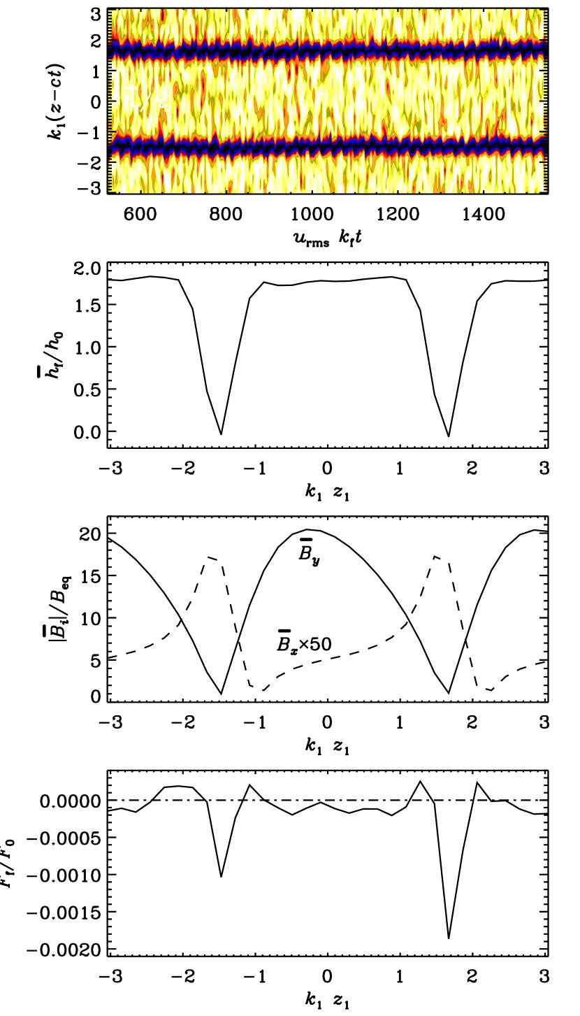
Figure 2.— Panel 1: visualization of $h_{\rm f}$ as a function of normalized $t$ and $z-ct$ for Run A: $k_{\rm f}/k_{1}=5$, $\mbox{\rm Re}=0.4$, $\mbox{\rm Re}_{M}=9$, and $\mbox{\rm Sh}=0.95$. Here $c=0.6\eta_{\rm t0}k_{1}$ is the actual speed of the dynamo wave. Panels 2–4 give the $z$ dependence of $h_{\rm f}$, $\overline{B}_{i}$ for $i=x$, $y$, and $\overline{F}$, averaged in the comoving frame over the time of the first panel.

The simulations developed the expected dynamo wave, so we analyze the data in a comoving frame in which the wave is standing, allowing us to average in time. In agreement with earlier work (Mitra et al., 2010; Hubbard & Brandenburg, 2010), the magnetic helicity of the small-scale magnetic field is then statistically steady and therefore the divergence of the magnetic helicity flux must be independent of the gauge chosen. Note that for Run A (Figure 2) the flux is generally quite small (less than $10^{-3}$ times the value expected based on equation 24), except when $\overline{B}_{y}=0$ where it shows a small peak. The situation is different in Runs B and C (Figures 3 and 4), where the flux is larger but uncorrelated compared to the spatial dependence expected to be dominated by $\overline{B}_{y}^{2}\gg\overline{B}_{x}^{2}$. Finally note that for a mean-field wavenumber $k=k_{1}$ the expected VC flux would be of wavenumber $2k_{1}$, not much smaller than forcing wavenumbers of $3k_{1}$ or $5k_{1}$. In Figure 5 we therefore present the results of Run D with $k_{\rm f}=20k_{1}$ in a non-cubic domain with $L_{z}=4L$. The results are qualitatively similar to Run A which has a similar $\mbox{\rm Re}_{M}$.

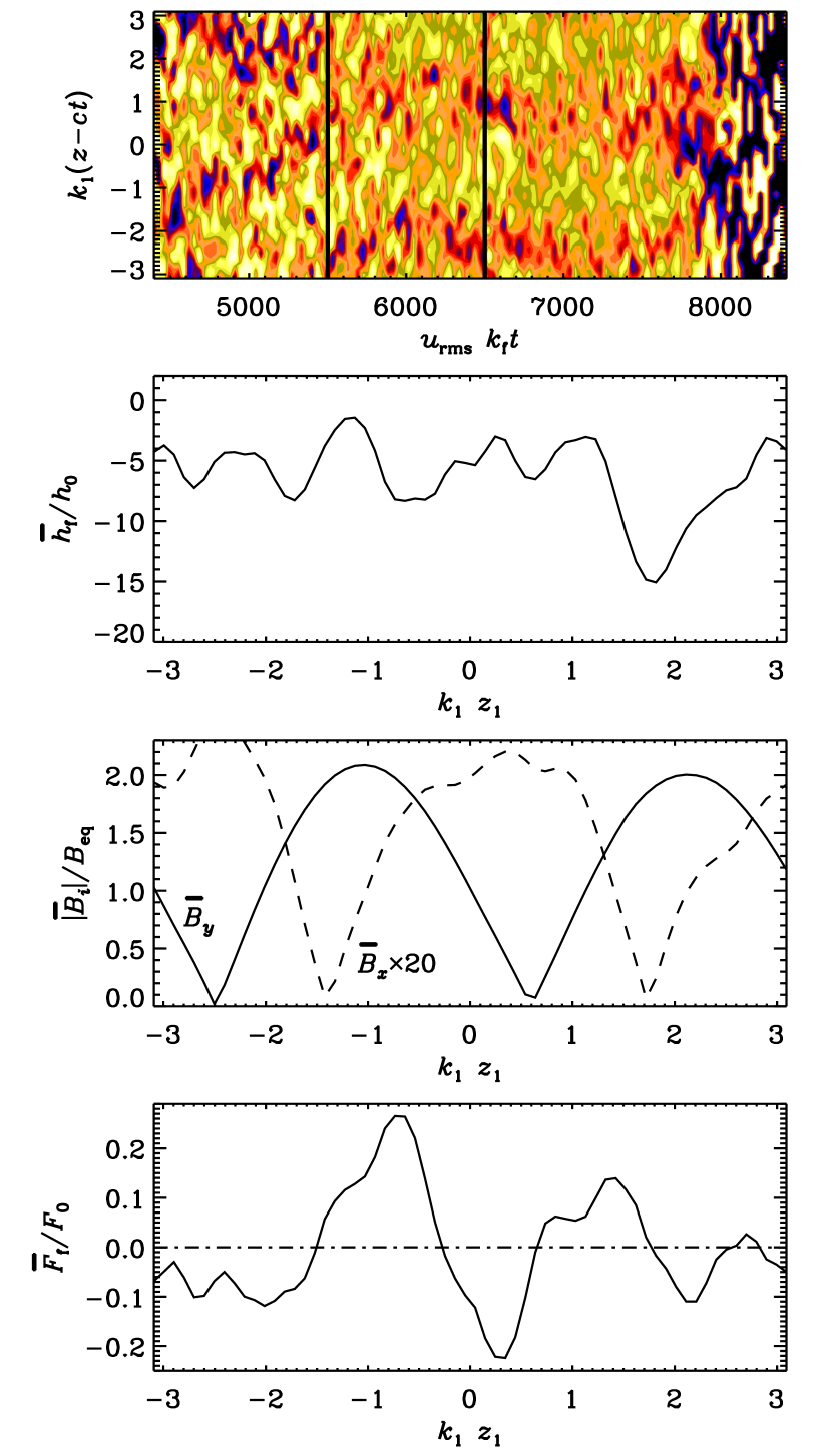
Figure 3.— Same as Figure 3, but for Run B: $k_{\rm f}/k_{1}=3$, $\mbox{\rm Re}=9$, $\mbox{\rm Re}_{M}=90$, and $\mbox{\rm Sh}=0.5$. In this case, $c=1.04\eta_{\rm t0}k_{1}$. The vertical bars in the first panel denote the time interval over which the functions in the other 3 panels are averaged. Note also that after $u_{\rm rms}k_{\rm f}t\approx 7800$ the dominant dynamo mode changes and the field becomes $x$ dependent.

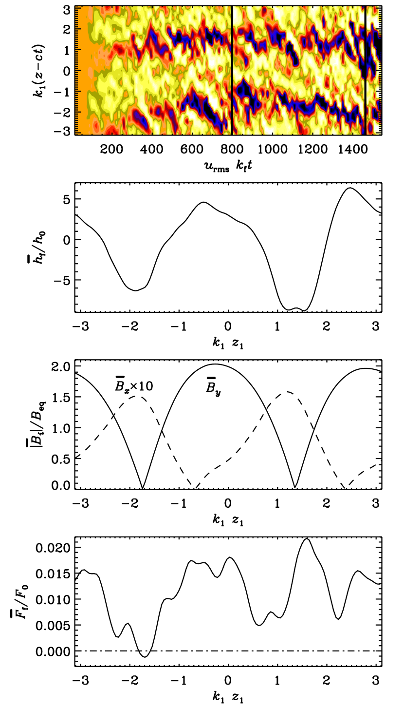
Figure 4.— Same as Figure 3, but for Run C: $k_{\rm f}/k_{1}=3$, $\mbox{\rm Re}=19$, $\mbox{\rm Re}_{M}=280$, and $\mbox{\rm Sh}=0.4$. The vertical bars in the first panel denote the time interval over which the functions in the other 3 panels are averaged.

The significant result to draw from the figures is that the small-scale flux is both smaller than the expected $\overline{\bm{F}}_{\text{VC}}$ and uncorrelated with it. Note that as the $y$-directed field is much greater than the $x$-directed field, as expected, and that the VC flux is approximately proportional to the square of the $\overline{B}_{y}$. Thus, according to our present results we must conclude that there is no support for the validity of Equation (24).

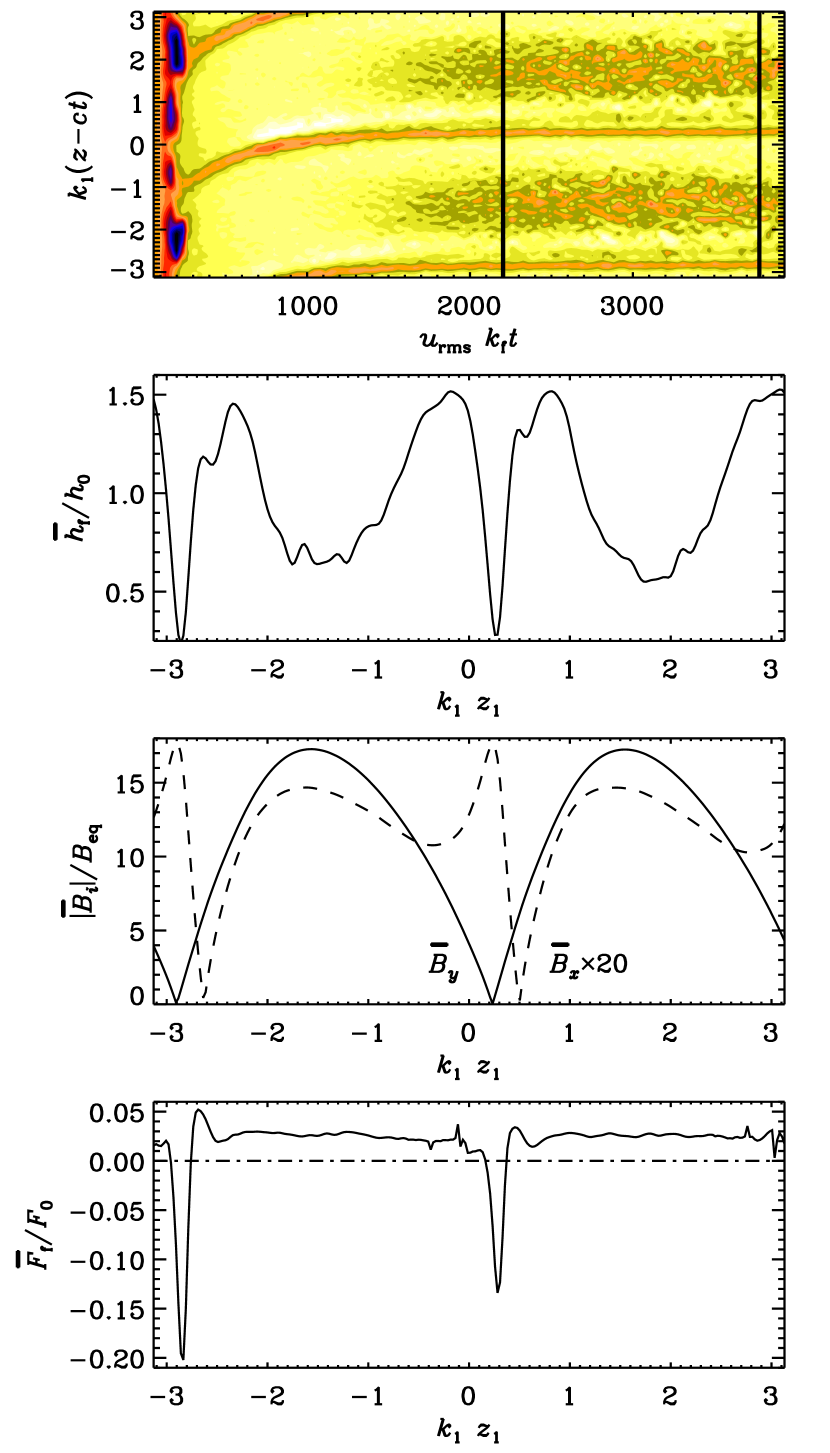
Figure 5.— Same as Figure 3, but for Run D: $k_{\rm f}/k_{1}=20$, $\mbox{\rm Re}=9$, $\mbox{\rm Re}_{M}=7.9$, and $\mbox{\rm Sh}=0.016$. The domain for this run is $\pi/2\times\pi/2\times 2\pi$, and the helicity in the top panel has been multiplied by 10 to achieve dynamic color range. The vertical bars in the first panel denote the time interval over which the functions in the other 3 panels are averaged.

6. Comparison with previous work

We would like to emphasize that our results are not in contradiction with previous calculations: we are not working in a gauge where one would expect the VC flux to exist. Disentangling the differing components (there are four in Subramanian & Brandenburg 2006, including an unexplored triple correlator) is not straightforward. In this work we are using the gauge independence of the divergence of the flux of small-scale magnetic helicity, as described in Section 2.2, to relate the observations in the shearing-advective gauge to the expected divergence of $\overline{\bm{F}}_{\text{VC}}$.

To date, the only numerical evidence for the VC flux comes from interpretations of the differing dynamo behavior in shearing systems with vertical field boundary conditions (that allow a flux) as compared with those systems with perfect conductor boundary conditions that disallow a flux; see Equation (6). Examples of such indirect evidence include the papers by Brandenburg (2005) and Käpylä et al. (2008). An alternative interpretation might simply be that the excitation condition for the onset of large-scale dynamo action are simply delayed sufficiently when changing the boundary condition from a vertical field to a perfect conductor condition, as was discussed also by Käpylä et al. (2010). It should also be noted that the use of $\overline{\bm{F}}_{\text{VC}}$ in various dynamical quenching models has not alleviated catastrophic quenching unless $C_{\text{VC}}$ is increased beyond a certain limit where the flux divergence leads to a magnetic $\alpha$ effect that is more important than the kinematic $\alpha$ effect (Brandenburg & Subramanian, 2005b; Guerrero et al., 2010); see also Appendix 5.2.

7. Conclusions

We conclude that there is at present no evidence for a shear-driven vertical flux of small-scale magnetic helicity in a gauge where the only significant flux must be vertical. We speculate that the finite divergence of the VC flux found earlier in analytic studies using Coulomb and related gauges might be a consequence of the gauge choice, which can generate unexpected horizontal helicity fluxes that are not normally considered. When the gauge choice is such that those horizontal fluxes are transformed out, there is no remaining vertical flux. It appears therefore that the VC flux does either not operate, or it at least does not follow the expected functional form. We note that diffusive fluxes have been found to exist, so there do remain mechanisms that can export small-scale magnetic helicity from a dynamo.

The simultaneous export of large- and small-scale helicity at some relative level is inevitable (Blackman & Brandenburg, 2003) and in fact necessary, because otherwise simple considerations (Brandenburg et al., 2002; Brandenburg & Subramanian, 2005a) have long suggested that the magnetic energy would reach unrealistically large values. The VC flux was a particularly promising mechanism to export small-scale magnetic helicity because it could do so while allowing the system to retain much of the large-scale dynamo generated field, resulting in rapid growth to strong mean fields. Turbulent diffusion of magnetic helicity is now the most promising escape from catastrophic $\alpha$ quenching – even for shearing systems. Simulation and theory suggest that this will be significant starting near $\mbox{\rm Re}_{M}=10^{4}$ (Mitra et al., 2010; Hubbard & Brandenburg, 2010), which, while astrophysically significant eludes numerical verification at present. However, diffusive fluxes must inevitably export scales of helicity at comparable fractional rates, reducing expected final field strengths below those that might have been hoped for with the VC flux.

References

- Blackman & Brandenburg (2002) Blackman, E. G., & Brandenburg, A., 2002, ApJ, 579, 359
- Blackman & Brandenburg (2003) Blackman, E. G., & Brandenburg, A., 2003, ApJ, 584, L99
- Brandenburg (2001) Brandenburg, A. 2001, ApJ, 550, 824
- Brandenburg (2005) Brandenburg, A. 2005, ApJ, 625, 539
- Brandenburg & Dobler (2001) Brandenburg, A., & Dobler, W. 2001, A&A, 369, 329
- Brandenburg & Sokoloff (2002) Brandenburg, A., & Sokoloff, D., 2002, Geophys. Astrophys. Fluid Dyn., 96, 319
- Brandenburg & Subramanian (2005a) Brandenburg, A., & Subramanian, K. 2005a, Phys. Rep., 417, 1
- Brandenburg & Subramanian (2005b) Brandenburg, A., & Subramanian, K. 2005b, Astron. Nachr., 326, 400
- Brandenburg et al. (2009) Brandenburg, A., Candelaresi, S., & Chatterjee, P. 2009, MNRAS, 398, 1414
- Brandenburg et al. (2002) Brandenburg, A., Dobler, W., & Subramanian, K. 2002, Astron. Nachr., 323, 99
- Brandenburg et al. (1995) Brandenburg, A., Nordlund, Å., Stein, R. F., & Torkelsson, U. 1995, ApJ, 446, 741
- Brandenburg et al. (2001) Brandenburg, A., Bigazzi, A., & Subramanian, K. 2001, MNRAS, 325, 685
- Brandenburg et al. (2008) Brandenburg, A., Rädler, K.-H., Rheinhardt, M., & Käpylä, P. J. 2008, ApJ, 676, 740
- Field & Blackman (2002) Field, G. B., & Blackman, E. G. 2002, ApJ, 572, 685
- Guerrero et al. (2010) Guerrero, G., Chatterjee, P., & Brandenburg, A., 2010, MNRAS, submitted arXiv:1005.4818
- Hubbard & Brandenburg (2010) Hubbard, A., & Brandenburg, A., 2010, Geophys. Astrophys. Fluid Dyn., in press, arXiv:1004.4591
- Käpylä & Brandenburg (2009) Käpylä, P. J., & Brandenburg, A. 2009, ApJ, 699, 1059
- Käpylä et al. (2008) Käpylä, P. J., Korpi, M. J., & Brandenburg, A. 2008, A&A, 491, 353
- Käpylä et al. (2010) Käpylä, P. J., Korpi, M. J., & Brandenburg, A. 2010, MNRAS, in press, arXiv:0911.4120
- Kleeorin & Ruzmaikin (1982) Kleeorin, N. I., & Ruzmaikin, A. A. 1982, Magnetohydrodynamics, 18, 116
- Kleeorin & Rogachevskii (1999) Kleeorin, N., & Rogachevskii, I. 1999, Phys. Rev. E, 59, 6724
- Krause & Rädler (1980) Krause, F., & Rädler, K.-H. 1980, Mean-field magnetohydrodynamics and dynamo theory (Pergamon Press, Oxford)
- Mitra et al. (2010) Mitra, D., Candelaresi, S., Chatterjee, P., Tavakol, R., & Brandenburg, A. 2010, Astron. Nachr., 331, 130
- Moffatt (1978) Moffatt, H. K. 1978, Magnetic field generation in electrically conducting fluids (Cambridge University Press, Cambridge)
- Rüdiger & Hollerbach (2004) Rüdiger, G., & Hollerbach, R. 2004, The magnetic universe (Wiley-VCH, Weinheim)
- Subramanian & Brandenburg (2004) Subramanian, K., & Brandenburg, A. 2004, Phys. Rev. Lett., 93, 205001
- Subramanian & Brandenburg (2006) Subramanian, K., & Brandenburg, A. 2006, ApJ, 648, L71
- Vishniac & Cho (2001) Vishniac, E. T., & Cho, J. 2001, ApJ, 550, 752
- Wisdom & Tremaine (1988) Wisdom, J., & Tremaine, S. 1988, AJ, 95, 925