Phase coexistence in congested states of pedestrian dynamics

Abstract

Experimental results for congested pedestrian traffic are presented. For data analysis we apply a method providing measurements on an individual scale. The resulting velocity-density relation shows a coexistence of moving and stopping states revealing the complex structure of pedestrian fundamental diagrams and supporting new insights into the characteristics of pedestrian congestions. Furthermore we introduce a model similar to event driven approaches. The velocity-density relation as well as the phase separation is reproduced. Variation of the parameter distribution indicates that the diversity of pedestrians is crucial for phase separation.

1 Introduction

The velocity-density relation is one of the most important characteristics for the transport properties of any traffic system. For pedestrian traffic there is currently no consensus even about the principle shape of this relation which is reflected e.g. in conflicting recommendations in various handbooks and guidelines [1]. Discrepancies occur in particular in the high-density regime which is also the most relevant for applications in safety analysis like evacuations or mass events. At high densities stop-and-go waves occur indicating overcrowding and potentially initiating dangerous situations due to stumbling etc. However, the densities where the flow breaks down due to congestion ranges from densities of $\rho_{\rm max}=3.8$ m^-2 to $\rho_{\rm max}=10$ m^-2 [1]. This large variation in values for $\rho_{\rm max}$ reported in the literature is partly due to insufficient methods of data capturing and data analysis. In previous experimental studies, different kinds of measurement methods are used and often a mixture of time and space averages are realized. Especially in the case of spatial and temporal inhomogeneities the choice of the measurement method and the type of averaging have a substantial influence on the results [2].

Up to now, congested states in pedestrian dynamics have not been analyzed in much detail. This is in contrast to vehicular traffic where the congested phase is well-investigated, both empirically and theoretically [3, 4].

In this contribution we show that even improved classical measurement methods using high precision trajectories but basing on mean values of density and velocity fail to resolve important characteristics of congested states. For a thorough analysis of pedestrian congestion we apply a new method enabling measurements on the scale of single pedestrians.

2 Experimental data

For our investigation we use data from experiments performed in 2006 in the wardroom of Bergische Kaserne Düsseldorf with a test group of up to $N=70$ soldiers. The length of the circular system was about 26 m, with a $l=4$ m long measurement section. Detailed information about the experimental setup and data capturing providing trajectories of high accuracy ($|x_{\rm err}|\leq 0.02$ m) is given in [2, 5].

Figure 1: Trajectories for the runs with $N=39,56,62$ and $70$ (left to right, top to bottom). With increasing density the occurrence of stop-and-go waves accumulate.

In Fig. 1 the $x$-component of trajectories is plotted against time. For the extraction of the trajectories, the pedestrians’ heads were marked and tracked. Backward movement leading to negative velocities is caused by head movement of the pedestrians during a standstill. Inhomogeneities in the trajectories increase with increasing density. As in vehicular traffic, jam waves propagating opposite to the movement direction (upstream) occur at higher densities.

Stopping is first observed during the runs with $N=45$ pedestrians, at $70$ pedestrians they can hardly move forward. Macroscopically one observes separation into a stopping area and an area where pedestrians walk slowly. In the following we analyze how macroscopic measurements blur this phase separation and apply a technique introduced in [6] enabling a measurement of the fundamental diagram on a ‘microscopic’ scale.

2.1 Macroscopic measurement

Speed $v_{i}$ of pedestrian $i$ and the associated density $\rho_{i}$ are calculated using the entrance and exit times $t_{i}^{\rm in}$ and $t_{i}^{\rm out}$ into and out of a measurement section of length $l_{m}=2$ m,

$$v_{i}=\frac{l_{m}}{t_{i}^{\rm out}-t_{i}^{\rm in}},\qquad\rho_{i}=\frac{1}{t_{i}^{\rm out}-t_{i}^{\rm in}}\int_{t_{i}^{\rm in}}^{t_{i}^{\rm out}}\rho(t)\,dt\quad\mbox{with}\quad\rho(t)=\frac{\sum{\Theta_{i}(t)}}{l_{m}}\,.$$ (1)

Figure 2: Velocity-density relation using an improved macroscopic measurement method. There is no indication of phase separation since stopping states ($v\approx 0$) occur only at large densities where no moving states ($v>0$) are observable.

The speed $v_{i}$ is a mean value over the space-time interval $\Delta t_{i}=t_{i}^{\rm out}-t_{i}^{\rm in}$ and $\Delta x=l_{m}$. By integration over the instantaneous density $\rho(t)$ the density is assigned to the same space-time interval. To reduce the fluctuations of $\rho(t)$ we use the quantity $\Theta_{i}(t)$, introduced in [7], which measures the fraction of space between pedestrians $i$ and $i+1$ that is inside the measurement area.

Results of the macroscopic measurement method are shown in Fig. 2. In comparison to method B introduced in [2] (see Fig. 6 of [2] which uses data based on the same trajectories as this study) the scatter of the data is reduced due to an improved density definition and a better assignment of density and velocity. However the resulting velocity-density relation does not allow to identify phase-separated states although these are clearly visible in the trajectories.

2.2 Microscopic measurement

To identify phase separated states we determine the velocity-density relation on the scale of single pedestrians. This can be achieved by the Voronoi density method [6]. In one dimension a Voronoi cell is bounded by the midpoints $z_{i}=({x_{i+1}+x_{i}})/{2}$ of the pedestrian positions $x_{i}$ and $x_{i+1}$. With the length $L_{i}=z_{i}-z_{i-1}$ of the Voronoi cell corresponding to pedestrian $i$ and $\Delta t=0.5$ s we define the instantaneous velocity and density by

$$v^{\prime}_{i}(t)=\frac{x_{i}(t+\Delta t/2)-x_{i}(t-\Delta t/2)}{\Delta t},\;\rho^{\prime}_{i}(x)=\left\{\begin{array}[]{r@{\quad:\quad}l}{1}/{L_{i}}&x\in[z_{i},z_{i+1}[\\ 0&\mbox{otherwise}\end{array}\right.\,.$$ (2)

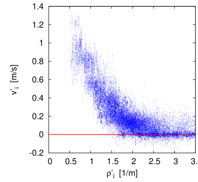
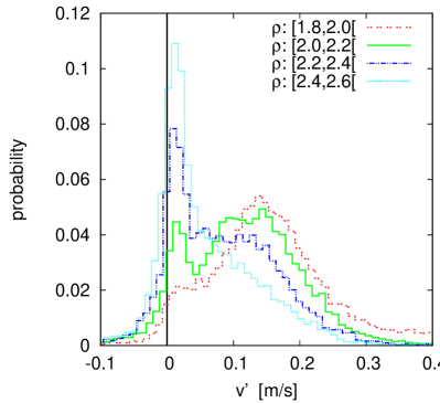
Figure 3: Left: Velocity-density relation on an individual scale. At each density $\rho^{\prime}>1.5~{}$m^-1 both stopping and moving states are observable. Right: Probability distribution of the velocities for different density intervals. The double peak structure indicates the coexistence of moving and stopping states. The height of the stopping peak increases with increasing density.

The fundamental diagram based on the Voronoi method is shown on the left side of Fig. 3. Regular stops occur at densities higher than 1.5 m^-1. On the right side of Fig. 3 the distribution of the velocities for fixed densities from 1.8 m^-1 to 2.6 m^-1 are shown. There is a continuous change from a single peak near $v=0.15~{}$m/s, to two peaks, to a single peak near $v=0~{}$m/s. The right peak represents the moving phase, whereas the left peak represents the stopping phase. At densities around 2.2 m^-1 these peaks coexist, indicating phase separation into a flowing and a jammed phase.

2.3 Phase separation in vehicular traffic

In highway traffic, phase separation into moving and stopping phases typically occurs when the outflow from a jam is reduced compared to maximal possible flow in the system. Related phenomena are hysteresis and a non-unique fundamental diagram. At intermediate densities two different flow values can be realized. The larger flow, corresponding to a homogeneous state, is metastable and breaks down due to fluctuations or perturbations (capacity drop). The origin of the reduced jam outflow is usually ascribed to the so-called slow-to-start behaviour (see [3, 4] and references therein), i.e. an delayed acceleration of stopped vehicles due to the loss of attention of the drivers etc.

The structure of the phase-separated states in vehicular traffic is different from the ones observed here. For vehicle traffic the stopping phase corresponds to a jam of maximal density whereas in the moving phase the flow corresponds to the maximal stable flow, i.e. all vehicles in the moving phase move at their desired speed. This scenario is density-independent as increasing the global density will only increase the length of the stopping region without reducing the average velocity in the free flow regime. The probability distribution of the velocities (in a periodic system) shows a similar behaviour to that observed in Fig. 3. The position of the free flow peak in the case of vehicular traffic is independent of the density.

The behaviour observed here for pedestrian dynamics differs slightly from that described above. The main difference concerns the properties of the moving regime. Here the observed average velocities are much smaller than the free walking speeds. Therefore the two regimes observed in the phase separated state are better characterized as “stopping” and “slow moving” regimes.

Further empirical studies are necessary to clarify the origin of these differences. One possible reason are the different acceleration properties of vehicles and pedestrians as well as anticipation effects. It also remains to be seen whether in pedestrian systems phenomena like hysteresis can be observed.

3 Modeling

3.1 Adaptive Velocity Model

In this section we introduce the adaptive velocity model, which is based on an event driven approach [9]. A pedestrian can be in different states which determine the velocity. A change between these states is called event. The model was derived from force-based models, where the dynamics of pedestrians are given by the following system of coupled differential equations

$$m_{i}\frac{dv_{i}}{dt}=F_{i}\quad\quad\mbox{with}\quad F_{i}=F_{i}^{\rm drv}+F_{i}^{\rm rep}\quad\mbox{and}\quad\frac{dx_{i}}{dt}=v_{i},$$ (3)

where $F_{i}$ is the force acting on pedestrian $i$. The mass is denoted by $m_{i}$, the velocity by $v_{i}$ and the current position by $x_{i}$. $F_{i}$ is split into a repulsive force $F_{i}^{\rm rep}$ and a driving force $F_{i}^{\rm drv}$. The dynamics is regulated by the interrelation between driving and repulsive forces. In our approach the role of repulsive forces are replaced by events. The driving force is defined as

$$F_{i}^{\rm drv}=\frac{v_{i}^{0}-v_{i}}{\tau_{i}},$$ (4)

where $v_{i}^{0}$ is the desired speed of a pedestrian and $\tau$ the relaxation time of the velocity. By solving the differential equation

$$\frac{dv_{i}}{dt}=F_{i}^{\rm drv}\quad\Rightarrow\quad v_{i}(t)=v_{i}^{0}+c\exp\left(-\frac{t}{\tau_{i}}\right),\quad\mbox{with }c\in\mathbb{R},$$ (5)

the velocity function is obtained. This is shown in Fig. 4 together with the parameters governing the pedestrians’ movement.

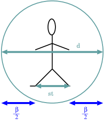
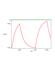
Figure 4: Left: Connection between the required space $d$, the step length $st$ and the safety distance $\beta$. Right: The adaptive velocity: acceleration until $t_{\rm dec1}$ than deceleration until $t_{\rm acc1}$, again acceleration until $t_{\rm dec2}$ and so on.

In this model pedestrians are treated as bodies with diameter $d$ [9]. The diameter depends linearly on the current velocity and is equal to the step length $st$ in addition to the safety distance $\beta$

$$d_{i}(t)=st_{i}(t)+\beta_{i}(t)$$ (6)

Step length and safety distance are introduced to define the rules for the dynamics of the system. We determine the model parameters from empirical data which allows to judge the adequacy of the rules. Based on [10] the step length is a linear function of the current velocity with following parameters:

$$st_{i}(t)=0.235m+0.302[s]\;v_{i}(t).$$ (7)

The required quantities for the safety distance can be specified through empirical data of the fundamental diagram $\bar{d}_{i}=1/\rho=0.36+1.06\;v$, see [7]. With these experimental results the previous equations can be summarized to

$$\beta_{i}(t)=d_{i}(t)-st_{i}(t)=a_{i}+b_{i}\;v_{i}(t)$$ (8)

with $a_{i}=0.125$ m and $b_{i}=0.758$ s. No free model parameter remain with these specifications. In the following we describe the rules for the movement. A pedestrian accelerates to the desired velocity $v_{i}^{0}$ until the distance $\Delta x_{i,i+1}$ to the pedestrian in front is smaller than the safety distance. From this time on, he/she decelerates until the distance is larger than the safety distance. To guarantee a minimal volume exclusion, case “collision” is included, in which the pedestrians are too close to each other and have to stop. Via $\Delta x_{i,i+1}$, $d_{i}$ and $\beta_{i}$ the velocity function for the states deceleration (dec.), acceleration (acc.) and collision (coll.) can be defined, see Eq. 9:

$$v_{i}(t)=\left\{\begin{array}[]{ccll}v_{\rm dec}\,\exp\left(-\frac{t-t_{\rm dec}}{\tau}\right)&\quad\mbox{for}&\Delta x_{i,i+1}-\delta_{i}(t)\leq 0&\quad\mbox{(dec.)}\\ \\ v_{i}^{0}(1-\exp\left(-\frac{t-t_{0}}{\tau}\right)&\quad\mbox{for}&\Delta x_{i,i+1}-\delta_{i}(t)>0&\quad\mbox{(acc.)}\\ \\ 0&\quad\mbox{for}&\Delta x_{i,i+1}-\delta_{i}(t)\leq-\beta_{i}(t)/2&\quad\mbox{(coll.)}\\ \end{array}\right.$$ (9)

where $\delta_{i}(t)=(d_{i}(t)+d_{i+1}(t))/2$ is the distance between the centers of both pedestrians. The current velocity $v_{i}(t)$ of an pedestrian $i$ depends on his/her state. $t_{\rm dec}$ denominates the point in time where a change from acceleration to deceleration takes place. Conversely $t_{\rm acc}$ is the change from deceleration to acceleration. $v_{\rm dec}=v(t_{\rm dec})$ and $v_{\rm acc}=v(t_{\rm acc})$ are defined accordingly. At the beginning $t_{0}=0$ s with a change from acceleration to deceleration a new calculation of $t_{0}$ is necessary:

$$t_{0}=t_{acc}+\ln\left(1-\frac{v_{\rm acc}}{v_{0}}\exp\left(\frac{-t_{\rm acc}-t_{\rm dec}}{\tau}\right)\right)$$ (10)

The discreteness of the time step could lead to configurations where overlapping occurs. To ensure good computational performance for high densities, no events are explicitly calculated. Instead in each time step, it is checked whether an event has taken place and $t_{\rm dec}$, $t_{\rm acc}$ or $t_{\rm coll}$ are set to $t$ accordingly. To avoid too large interpenetration of pedestrians and to implement a reaction time in a realistic size we choose $\Delta t=0.05$ s. To guarantee a parallel update a recursive procedure is necessary: Each person is advanced one time step according to Eq. 9. If after this step a pedestrian is in a different state because of the new distance to the pedestrian in front, the velocity is set according to this state. Then the state of the next following person is reexamined. If the state is still valid the update is completed. Otherwise, the velocity is calculated again.

3.2 Model validation and influence of individual differences

In the following we face model results with experimental data and study how the distribution of individual parameter influences the phase separation. For all simulations the desired velocity is normal distributed $v_{i}^{0}\sim\mathcal{N}(\mu,\sigma^{2})$ with average $\mu=1.24$ m/s and variance $\sigma^{2}=0.05$. Fig. 5 and Fig. 6 show the simulation results for two different choices of parameter distributions.

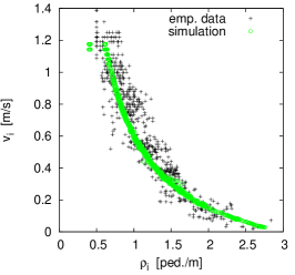
Figure 5: Validation of the modeled fundamental diagram and trajectories with same parameter $a_{i}$, $b_{i}$ and $\tau_{i}$ for all pedestrians Left: Comparison of fundamental diagrams of modeled and empirical data. Middle: Trajectories for $N=62$ (model). Right: Trajectories for $N=70$ (model).

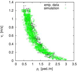
Figure 6: Validation of the modeled fundamental diagram and trajectories, with normal distributed individual parameter. Left: Comparison of fundamental diagrams of modeled and empirical data. Middle: Trajectories for $N=62$ (model). Right: Trajectories for $N=70$ (model).

The model yields the right macroscopic relation between velocity and density even if $a_{i},b_{i},st_{i}$ and $\tau_{i}$ are the same for all pedestrians, see Fig. 5 (left). The trajectories display that phase separation does not appear. Even at high densities the movement is ordered and no stops occur. For further simulations we incorporate a certain disorder by choosing the following individual parameter normal distributed: $a_{i}\sim\mathcal{N}(0.125,0.1)$, $b_{i}\sim\mathcal{N}(0.758,0.5)$ and $\tau_{i}\sim\mathcal{N}(1.0,0.1)$.

Variation of the personal parameters affects the scatter of the fundamental diagram, see Fig. 6, left. Phase separation appears in the modeled trajectories as in the experiment, see Fig. 6 middle and right. It is clearly visible that long stop phases occur by introducing distributed individual parameters. Then the pattern as well as the change of the pattern from $N=62$ to $N=70$ are in good agreement with the experimental results, see Fig. 1. Even the phase separated regimes match qualitatively. However, the regimes appear more regular in the modeled trajectories.

In Fig. 7 microscopic measurements of fundamental diagram and the related velocity distributions are shown. Separation of phases is reproduced well. But the position of the peak attributed to the moving phase is not in conformance with the experimental data, compare Fig. 3 (right). The experimental data show that the peak position is independent from the density at $v$ around $0.15$ m/s. At the model data the position of the peak changes with increasing density. Measurements with different time steps show that the size of the time step influences the length and shape of the stop phase at high densities. But the density where first stops occur seems independent from the size of the time step. Further model analysis is necessary to study the role of the reaction time implemented by discrete time steps in this special type of update. Furthermore we will study how the change of the peak could be influenced by including a distribution for the step length and other variations of the distribution for the safety distance.

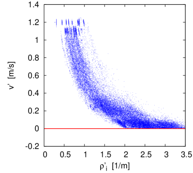
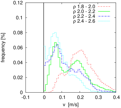
Figure 7: Left: Microscopic fundamental diagram of the modeled data with normal distributed individual parameters. Right: Distribution of $v$ at fixed densities.

4 Conclusion

We have investigated the congested regime of pedestrian traffic using high-quality empirical data based on individual trajectories. Strong evidence for phase separation into standing and slow moving regimes is found. The corresponding velocity distributions show a typical two-peak structure. The structure of the trajectories is well reproduced by an adaptive velocity model which is a variant of force-based models in continuous space.

Future studies should clarify the origin of the differences to the phase separated states observed in vehicular traffic. Here phase separation into a stopping and a moving phase occurs such that the average velocity in the moving regime is independent of the total density.

Acknowledgments.

This work is supported by the Federal Ministry of Education and Research - BMBF (FKZ 13N9952 and 13N9960) and by the German Research Foundation - DFG (KL 1873/1-1 and SE 1789/1-1).

References

- [1] Schadschneider, A., Klingsch, W., Klüpfel, H., Kretz, T., Rogsch, C., Seyfried, A.: Evacuation Dynamics: Empirical Results, Modeling and Applications, In: Meyers R. A. (Ed.), Encyclopedia of Complexity and System Science, pp. 3142-3176. Springer (2009)
- [2] Seyfried, A., Boltes, M., Kähler, J., Klingsch, W., Portz, A., Schadschneider A., Steffen, B., Winkens, A.: Enhanced empirical data for the fundamental diagram and the flow through bottlenecks. In: Klingsch, W.W.F., Rogsch, C., Schadschneider, A. and M. Schreckenberg (Eds.), Pedestrian and Evacuation Dynamics 2008, pp. 145-156, Springer (2010)
- [3] Chowdhury, D., Santen, L., Schadschneider, A.: Statistical physics of vehicular traffic and some related systems. Phys. Rep. 329, 199 (2000)
- [4] Schadschneider, A., Chowdhury, D., Nishinari, K.: Stochastic Transport in Complex Systems. Elsevier (2010)
- [5] Boltes, M., Seyfried, A., Steffen, B. and Schadschneider, A.: Automatic Extraction of Pedestrian Trajectories from Video Recordings. In: Klingsch, W.W.F., Rogsch C., Schadschneider A. and M. Schreckenberg (Eds.), Pedestrian and Evacuation Dynamics 2008, pp. 43-54, Springer (2010)
- [6] Steffen, B. and Seyfried, A.: Methods for measuring pedestrians density, flow, speed and direction with minimal scatter. Physica A 389, 1902-1910 (2010)
- [7] Seyfried, A., Steffen, B., Klingsch, W. and Boltes, M.: The fundamental diagram of pedestrian movement revisited. J. Stat. Mech., P10002 (2005)
- [8] Portz, A. and Seyfried, A.: Analyzing Stop-and-Go Waves by Experiment and Modeling. Pedestrian and Evacuation Dynamics 2010, to appear. Preprint arxiv:1003.5446v1 (2010)
- [9] Chraibi, M. and Seyfried, A.: Pedestrian Dynamics With Event-driven Simulation. In: Pedestrian and Evacuation Dynamics 2008, pp. 713-718, Springer (2010)
- [10] Weidmann, U.: Transporttechnik der Fussgänger. Schriftenreihe des IVT Nr. 90, Institut für Verkehrsplanung, Transporttechnik, Strassen- und Eisenbahnbau, ETH, Zürich (1993)