Anomalous Andreev bound state in non-centrosymmetric superconductors

Abstract

We study edge states of non-centrosymmetric superconductors where spin-singlet $d$-wave pairing mixes with spin-triplet $p$ (or $f)$-wave one by spin-orbit coupling. For $d_{xy}$-wave pairing, the obtained Andreev bound state has an anomalous dispersion as compared to conventional helical edge modes. A unique topologically protected time-reversal invariant Majorana bound state appears at the edge. The charge conductance in the non-centrosymmetric superconductor junctions reflects the anomalous structures of the dispersions, particularly the time-reversal invariant Majorana bound state is manifested as a zero bias conductance peak.

Recently, physics of non-centrosymmetric (NCS) superconductors is one of the important issues in condensed matter physics Bauer ; Zheng ; Frigeri ; Interface . One of the remarkable features in NCS superconductors is that due to the broken inversion symmetry, superconducting pair potential becomes a mixture of spin-singlet even-parity and spin-triplet odd-parity Gorkov . Due to the mixture of spin-singlet and spin-triplet pairings, several novel properties such as the large upper critical field are expected Frigeri ; Fujimoto1 .

Up to now, there have been several studies about superconducting profiles of NCS superconductors Frigeri ; Fujimoto1 ; Yanase ; Linder ; Iniotakis ; Eschrig ; Tanaka ; Sato2009 ; Yip . In these works, pairing symmetry of NCS superconductors has been mainly assumed to be $s+p$-wave. However, in a strongly correlated system, this assumption is not valid anymore. Microscopic calculations have shown that $d_{x^{2}-y^{2}}$-wave spin-singlet pairing mixes with $f$-wave pairing based on the Hubbard model near half filling NCS-theory . Also, a possible pairing symmetry of superconductivity generated at heterointerface LaAlO₃/SrTiO₃ Interface has been studied based on a similar model Yada . It has been found that the gap function consists of spin-singlet $d_{xy}$-wave component and spin-triplet $p$-wave one Yada . Therefore, now, it is a challenging issue to reveal novel properties specific to $d_{xy}+p$ or $d_{x^{2}-y^{2}}+f$-wave pairing.

The generation of Andreev bound state(ABS) at the surface or interface is a significantly important feature specific to unconventional pairing since ABS directly manifests itself in the tunneling spectroscopy. Actually, for $d_{xy}$-wave pairing, zero energy dispersionless ABS appears ABS . The presence of ABS has been verified by tunneling experiments of high-T_c cuprate TK95 as a zero bias conductance peak (ZBCP). For NCS superconductors, when $p$-wave pair potential is larger than $s$-wave one, it has been shown that ABS is generated at its edge as helical edge modes similar to those in quantum spin Hall systemIniotakis ; Eschrig ; Tanaka ; Sato2009 . Several new features of spin transport stemming from these helical edge modes have been also predicted Eschrig ; Tanaka ; Sato2009 ; Yip . However, there has been no theory about ABS in $d_{xy}+p$- or $d_{x^{2}-y^{2}}+f$-wave pairing in NCS superconductors. Since tunneling spectroscopy via ABS ABS is a powerful method to identify pairing symmetry and mechanism of unconventional superconductors TK95 , it is quite important and interesting to clarify ABS and resulting tunneling conductance for $d_{xy}+p$-wave and $d_{x^{2}-y^{2}}+f$-wave pairings.

In this Letter, we investigate ABS and tunneling conductance $\sigma_{C}$ in normal metal / NCS superconductor junctions. For both $d_{xy}+p$-wave and $d_{x^{2}-y^{2}}+f$-wave cases, new types of ABS are obtained. In particular, for $d_{xy}+p$-wave case, due to the Fermi surface splitting by spin-orbit coupling, a single branch of topologically stable Majorana bound state appears. Recently, to search for Majorana fermions is one of the hottest issues in condensed matter physicsWilczek ; Majorana1 . In stark contrast to the other Majorana fermions, the present one preserves time-reversal symmetry. From this difference, the “time-reversal invariant (TRI) Majorana bound state” has a peculiar flat dispersion. It shows a unique ZBCP in $\sigma_{C}$ depending on the spin-orbit coupling. Therefore, the experimental identification is feasible.

We start with the Hamiltonian of NCS superconductor

$$\check{H}_{S}=\left({\begin{array}[]{*{20}c}{\hat{H}\left({\bf k}\right)}&{\hat{\Delta}\left({\bf k}\right)}\\ {-\hat{\Delta}^{*}\left({-{\bf k}}\right)}&{-\hat{H}^{*}\left({-{\bf k}}\right)}\\ \end{array}}\right)$$ (3)

with $\hat{H}({\bm{k}})=\xi_{{\bm{k}}}+\bm{V}(\bm{k})\cdot\hat{\bm{\sigma}}$, $\bm{V}({\bm{k}})=\lambda(\hat{\bm{x}}k_{y}-\hat{\bm{y}}k_{x})$, $\xi_{\bm{k}}=\hbar^{2}{\bm{k}}^{2}/(2m)-\mu$. Here, $\mu$, $m$, $\hat{\bm{\sigma}}$ and $\lambda$ denote chemical potential, effective mass, Pauli matrices and coupling constant of Rashba spin-orbit interaction, respectively Frigeri . The pair potential $\hat{\Delta}(\bm{k})$ is given by $\hat{\Delta}(\bm{k})=[\bm{d}(\bm{k})\cdot\hat{{\bm{\sigma}}}]i\hat{\sigma}_{y}+i\psi(\bm{k})\hat{\sigma}_{y}.$ Due to the spin-orbit coupling, the spin-triplet component $\bm{d}(\bm{k})$ is aligned with the polarization vector of the Rashba spin orbit coupling, $\bm{d}(\bm{k})||\bm{V}(\bm{k})$Frigeri . Then, the triplet component is $\bm{d}(\bm{k})=\Delta_{t}f({\bm{k}})(\hat{\bm{x}}k_{y}-\hat{\bm{y}}k_{x})/k$ with $k=\sqrt{{\bm{k}}^{2}}$ while singlet component reads $\psi(\bm{k})=\Delta_{s}f({\bm{k}})$ with $\Delta_{t}\geq 0$ and $\Delta_{s}\geq 0$. $f(\bm{k})$ is given by $f(\bm{k})=2k_{x}k_{y}/k^{2}$ for $d_{xy}+p$-wave and $f(\bm{k})=(k_{x}^{2}-k_{y}^{2})/k^{2}$ for $d_{x^{2}-y^{2}}+f$-wave.dxy The superconducting gaps are $\Delta_{1}=|\bar{\Delta}_{1}(\bm{k})|$ and $\Delta_{2}=|\bar{\Delta}_{2}(\bm{k})|$ for the two spin-split band with $\bar{\Delta}_{1}({\bm{k}})=(\Delta_{t}+\Delta_{s})f({\bm{k}})$ and $\bar{\Delta}_{2}({\bm{k}})=(\Delta_{t}-\Delta_{s})f({\bm{k}})$, respectively, in homogeneous state Iniotakis .

Let us consider a wave function including ABS localized at the surface. Consider a two-dimensional semi-infinite superconductor on $x>0$ where the surface is located at $x=0$. The corresponding wave function is given by Tanaka

$$\Psi_{S}(x)=[c_{1}^{+}\psi_{1}^{+}\exp(iq^{+}_{1x}x)+c_{1}^{-}\psi_{1}^{-}\exp(-iq^{-}_{1x}x)$$

$$+c_{2}^{+}\psi_{2}^{+}\exp(iq^{+}_{2x}x)+c_{2}^{-}\psi_{2}^{-}\exp(-iq^{-}_{2x}x)]\exp(ik_{y}y),$$ (4)

$$q^{\pm}_{1(2)x}=k^{\pm}_{1(2)x}\pm\frac{k_{1(2)}}{k^{\pm}_{1(2)x}}\sqrt{\frac{E^{2}-[\bar{\Delta}_{1(2)}(\bm{k}_{1(2)}^{\pm})]^{2}}{\lambda^{2}+2\hbar^{2}\mu/m}},$$

with $k^{+}_{1(2)x}=k^{-}_{1(2)x}=\sqrt{k_{1(2)}^{2}-k_{y}^{2}}$ for $|k_{y}|\leq k_{1(2)}$ and $k^{+}_{1(2)x}=-k^{-}_{1(2)x}=i\sqrt{k_{y}^{2}-k_{1(2)}^{2}}$ for $|k_{y}|>k_{1(2)}$, and $\bm{k}_{1(2)}^{\pm}=(\pm k_{1(2)x}^{\pm},k_{y})$. Here, $k_{1}$ and $k_{2}$ are the Fermi wavenumbers for the smaller and larger Fermi surface given by $-m\lambda/\hbar^{2}+\sqrt{(m\lambda/\hbar^{2})^{2}+2m\mu/\hbar^{2}}$ and $m\lambda/\hbar^{2}+\sqrt{(m\lambda/\hbar^{2})^{2}+2m\mu/\hbar^{2}}$, respectively. The wave functions are given by ${}^{T}\psi_{1}^{\pm}=\left(1,-i\alpha_{1\pm}^{-1},i\alpha_{1\pm}^{-1}\Gamma_{1\pm},\Gamma_{1\pm}\right)$ and ${}^{T}\psi_{2}^{\pm}=\left(1,i\alpha_{2\pm}^{-1},i\alpha_{2\pm}^{-1}\Gamma_{2\pm},-\Gamma_{2\pm}\right)$ with

$$\Gamma_{1(2)\pm}=\frac{\bar{\Delta}_{1(2)}(\bm{k}_{1(2)}^{\pm})}{E\pm\sqrt{E^{2}-[\bar{\Delta}_{1(2)}(\bm{k}_{1(2)}^{\pm})]^{2}}},$$ (5)

and $\alpha_{1(2)\pm}=(\pm k^{\pm}_{1(2)x}-ik_{y})/k_{1(2)}$. $E$ is the quasiparticle energy measured from the Fermi energy.

Postulating $\Psi_{S}(x)=0$ at $x=0$, we can determine the ABS. We consider the case for $|k_{y}|<k_{2}$. We first focus on the ABS for $d_{xy}+p$-wave case. For $\Delta_{t}>\Delta_{s}$, the dispersion $\varepsilon_{b}$ of ABS is given by

$$\displaystyle\varepsilon_{b}=\left\{\begin{array}[]{ll}\frac{\pm 2\Delta_{t}\gamma\sqrt{(k_{1}^{2}-k_{y}^{2})(k_{2}^{2}-k_{y}^{2})(k_{y}^{2}-\eta^{2}k_{1}^{2})}}{(k_{1}+k_{2})k_{1}k_{2}}&k_{c}<|k_{y}|\leq k_{1}\\ 0&k_{1}<|k_{y}|\end{array}\right.$$ (8)

with $\gamma=(k_{1}/k_{2}+k_{2}/k_{1})+(\Delta_{s}/\Delta_{t})(k_{2}/k_{1}-k_{1}/k_{2})$, $\eta=[\Delta_{t}(1-k_{1}/k_{2})+\Delta_{s}(1+k_{1}/k_{2})]/\{\Delta_{t}[1+(k_{1}/k_{2})^{2}]+\Delta_{s}[1-(k_{1}/k_{2})^{2}]\}$, $k_{c}=k_{1}\sqrt{\Delta_{t}(1-k_{1}/k_{2})+\Delta_{s}}/\sqrt{\Delta_{t}+\Delta_{s}[1-(k_{1}/k_{2})^{2}]}$. On the other hand, for $\Delta_{s}>\Delta_{t}$, the resulting $\varepsilon_{b}$ is given by $\varepsilon_{b}=0.$ The dispersion $\varepsilon_{b}$ of ABS changes drastically at $\Delta_{s}=\Delta_{t}$, where one of the energy gaps, i.e. $\Delta_{2}$, becomes zero. It should be remarked that the present ABSs do not break the time reversal symmetry.

The resulting $\varepsilon_{b}$ is plotted for various cases in Fig. 1 with $\Delta_{0}=\Delta_{s}+\Delta_{t}$. For convenience, we introduce dimensionless constant $\beta=2m\lambda/(\hbar^{2}k_{f})$ with $k_{f}=\sqrt{2m\mu/\hbar^{2}}$. We also plot $\Delta_{1}$ and $\Delta_{2}$. Both $\Delta_{1}$ and $\Delta_{2}$ become zero at $k_{y}=0$. At $|k_{y}|=k_{2}$, $\Delta_{2}$ is always zero. However, $\Delta_{1}$ then becomes zero only for $\beta=0$. First, we look at the $\Delta_{t}>\Delta_{s}$ case. For $\Delta_{s}=0$ with $\beta=0$, $\varepsilon_{b}=\pm ck_{y}$ with some constant $c$ for small $k_{y}$ (curve $a$ in Fig. 1(A)) as shown in the case of $s+p$-wave pairingLinder ; Iniotakis ; Eschrig ; Tanaka ; Sato2009 ; Yip since $\eta=0$ is satisfied. This type of ABS is called helical edge mode Tanaka ; Sato2009 ; Qi . However, this condition is satisfied only for $\Delta_{s}=0$ and $\beta=0$. In fact, $\varepsilon_{b}$ near $k_{y}=0$ becomes absent in general as shown in curves $a$ in Figs. 1(B), (D) and (E). At $k=\pm k_{c}$, $\varepsilon_{b}$ coincides with $\pm\Delta_{2}$. For nonzero $\beta$, $\varepsilon_{b}$ becomes exactly zero for $|k_{y}|>k_{1}$ as shown in curves $a$ in Figs. 1(D) and (E). The present line shapes of $\varepsilon_{b}$ are completely different from those of $s+p$-wave superconductors. On the other hand, for $\Delta_{s}>\Delta_{t}$, $\varepsilon_{b}=0$ for any $k_{y}$ similar to the case of spin-singlet $d_{xy}$ or spin-triplet $p_{x}$-wave pairing ABS ; TK95 .

We notice here that the zero energy bound state for $|k_{y}|>k_{1}$ is a Majorana bound state. The wave function for the zero energy edge state $\Psi_{m}(k_{y})$ can be written as ${}^{T}\Psi_{m}(k_{y})=(u_{1}(k_{y}),u_{2}(k_{y}),v_{1}(k_{y}),v_{2}(k_{y}))$ where

$$u_{1}(k_{y})=-i\sigma v_{2}(k_{y})=\frac{(\alpha f_{1}-\beta_{1}f_{2})\exp(ik_{y}y-i\frac{\pi}{4})}{\sqrt{\sigma\alpha}}$$ (9)

$$u_{2}(k_{y})=i\sigma v_{1}(k_{y})=\frac{(f_{1}+\beta_{2}f_{2})\exp(ik_{y}y-i\frac{\pi}{4})}{\sqrt{\sigma\alpha}}$$ (10)

with $\alpha=(k_{y}-\sqrt{k_{y}^{2}-k_{1}^{2}})/k_{1}$, $\beta_{1}=(\alpha k_{y}/k_{2}+1)$, $\beta_{2}=(\alpha+k_{y}/k_{2})$ and $\sigma={\rm sgn}(k_{y})$. The functions $f_{1}$ and $f_{2}$ decays exponentially as a function of $x$ and are even function of $k_{y}$. The Bogoliubov quasiparticle creation operator for this state is constructed in the usual way as $\gamma^{\dagger}(k_{y})=u_{1}(k_{y})c_{\uparrow}^{\dagger}(k_{y})+u_{2}(k_{y})c_{\downarrow}^{\dagger}(k_{y})+v_{1}(k_{y})c_{\uparrow}(-k_{y})+v_{2}(k_{y})c_{\downarrow}(-k_{y})$. Since $u_{1}(k_{y})=v_{1}^{*}(-k_{y})$ and $u_{2}(k_{y})=v_{2}^{*}(-k_{y})$ are satisfied, it is possible to verify that $\gamma^{\dagger}(k_{y})=\gamma(-k_{y})$. This means the generation of Majorana bound state at the edge for $|k_{y}|>k_{1}$. For $\Delta_{s}>\Delta_{t}$, a similar Majorana bound state also appears for $|k_{y}|>k_{1}$. On the other hand, for $|k_{y}|\leq k_{1}$, Majorana bound state has double branches and it is reduced to be conventional zero energy ABS.

Unlike Majorana fermions studied before Wilczek ; Majorana1 , the present single Majorana bound state is realized with time reversal symmetry. The TRI Majorana bound state has the following three characteristics. a) It has a unique flat dispersion: To be consistent with the time-reversal invariance, the single branch of zero mode should be symmetric under $k_{y}\rightarrow-k_{y}$. Therefore, by taking into account the particle-hole symmetry as well, the flat dispersion is required. On the other hand, the conventional time-reversal breaking Majorana bound state has a linear dispersion. b) The spin-orbit coupling is necessary to obtain the TRI Majorana bound state. Without spin-orbit coupling, the TRI Majorana bound state vanishes. c) The TRI Majorana bound state is topologically stable under small deformations of the Hamiltonian (3).

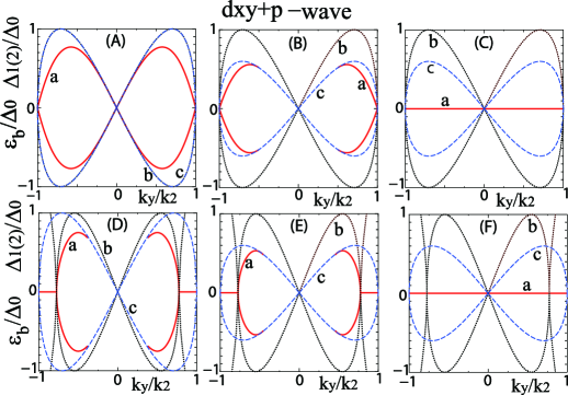
Figure 1: (Color online) Andreev bound state $\varepsilon_{b}$, effective pair potentials for each Fermi surface $\Delta_{1}$ and $\Delta_{2}$ are plotted for $d_{xy}+p$-wave case as a function of $k_{y}/k_{2}$. $\beta=0$ for panels A, B and C. $\beta=0.5$ for panels D, E and F. $\Delta_{t}=\Delta_{0}$, $\Delta_{s}=0$ for A and D. $\Delta_{t}=0.8\Delta_{0}$, $\Delta_{s}=0.2\Delta_{0}$ for B and E. $\Delta_{t}=0.2\Delta_{0}$, $\Delta_{s}=0.8\Delta_{0}$, for C and F. In all panels, curves a (solid line), b (dotted line) and c (dashed line) denote $\varepsilon_{b}/\Delta_{0}$, $\Delta_{1}/\Delta_{0}$ and $\Delta_{2}/\Delta_{0}$, respectively.

We also calculate ABS for $d_{x^{2}-y^{2}}+f$-wave case. In this case, ABS exists only for $\Delta_{s}<\Delta_{t}$. In Fig. 2, $\varepsilon_{b}$ is plotted similarly to Fig. 1. As a reference, corresponding $\varepsilon_{b}$ is also shown for $s+p$-wave case. Helical edge modes around $k_{y}=0$ exist and $\varepsilon_{b}$ is absorbed into continuum levels for $|k_{y}|>k_{1}$. These features are similar to those of $s+p$-wave case. However, the number of crossing points of $\varepsilon_{b}$ is five for $d_{x^{2}-y^{2}}+f$-wave case reflecting the complex ${\bm{k}}$-dependence of the pair potential. The overall line shapes of $\varepsilon_{b}$ (curve $a$) in Fig. 2(A) is significantly different from corresponding $\varepsilon_{b}$ (curve $a$) in Fig. 2(B).

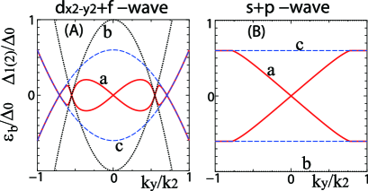
Figure 2: (Color online) Similar plots to Fig. 1 with $\beta=0.5$ for $d_{x^{2}-y^{2}}+f$-wave (A) and $s+p$-wave case (B) with $\Delta_{t}=0.8\Delta_{0}$, $\Delta_{s}=0.2\Delta_{0}$. In all panels, curves a(solid line), b(dotted line) and c(dashed line) denote $\varepsilon_{b}/\Delta_{0}$, $\Delta_{1}/\Delta_{0}$ and $\Delta_{2}/\Delta_{0}$, respectively.

It is very interesting to clarify how the above novel types of ABS are reflected in the charge transport property Iniotakis . The Hamiltonian $\check{H}_{N}$ in a normal metal is given by putting $\hat{\Delta}(\bm{k})=0$ and $\lambda=0$ in $\check{H}_{S}$. We assume an insulating barrier at $x=0$ expressed by a delta-function potential $U\delta(x)$. The wave function for spin $\gamma=(\uparrow,\downarrow)$ in the normal metal $\Psi_{N}(x)$ is given by

$$\Psi_{N}(x)\!\! = \!\!\exp(ik_{Fy}y)[(\psi_{i\gamma}+\sum_{\rho=\uparrow,\downarrow}a_{\gamma,\rho}\psi_{a\rho})\exp(ik_{Fx}x)$$ (11)

$$+\sum_{\rho=\uparrow,\downarrow}b_{\gamma,\rho}\psi_{b\rho}\exp(-ik_{Fx}x)]$$

with ${}^{T}\psi_{i\uparrow}$$=$ ${}^{T}\psi_{b\uparrow}$ $=$$\left(1,0,0,0\right)$, ${}^{T}\psi_{i\downarrow}$=${}^{T}\psi_{b\downarrow}$ $=$$\left(0,1,0,0\right)$, ${}^{T}\psi_{a\uparrow}$ $=$$\left(0,0,1,0\right)$, and ${}^{T}\psi_{a\downarrow}$ $=$$\left(0,0,0,1\right)$. The corresponding $\Psi_{S}(x)$ is given by Eq. (4). The coefficients $a_{\gamma,\rho}$ and $b_{\gamma,\rho}$ are determined by the boundary condition $\Psi_{N}(0)=\Psi_{S}(0)$, and $\hbar\check{v}_{Sx}\Psi_{S}(0)-\hbar\check{v}_{Nx}\Psi_{N}(0)=-2iU\check{\tau}_{3}\Psi_{S}(0)$ with $\hbar\check{v}_{S(N)x}=\partial\check{H}_{S(N)}/\partial k_{x}$, and diagonal matrix $\check{\tau}_{3}$ given by $\check{\tau}_{3}={\rm diag}(1,1,-1,-1)$.

The quantity of interest is the angle averaged charge conductance $\sigma_{C}$ given by

$$\sigma_{C}=\frac{\int^{\pi/2}_{-\pi/2}f_{C}(\phi)d\phi}{\int^{\pi/2}_{-\pi/2}f_{NC}(\phi)d\phi},$$ (12)

$$f_{C}(\phi)=[2+\sum_{\gamma,\rho}(\mid a_{\gamma,\rho}\mid^{2}-\mid b_{\gamma,\rho}\mid^{2})]\frac{\cos\phi}{2},$$ (13)

where $f_{NC}(\phi)$ denotes the angle resolved charge conductance in the normal state with $\hat{\Delta}({\bm{k}})=0$. Here, $\phi$ denotes the injection angle measured from the normal to the interface with $\sin\phi=k_{y}/k_{f}$. To characterize transparency of the junction interface, we introduce dimensionless constant $Z=2mU/\hbar^{2}k_{f}$.

We plot bias voltage $eV=E$ dependence of $\sigma_{C}$ for $d_{xy}+p$-wave case in Fig. 3 for various $Z$. First we concentrate on low transparent junction with $Z=5$ by changing the value of $\Delta_{s}$ and $\Delta_{t}$. At $\Delta_{t}=\Delta_{s}$, one of the energy gap of the Fermi surface closes corresponding to the quantum phase transition. Then, the resulting $\sigma_{C}$ has a gradual change from the quantum critical point.

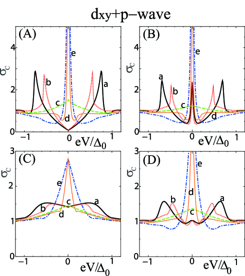
Figure 3: (Color online) Tunneling conductance $\sigma_{C}$ for $d_{xy}+p$-wave case. A: $Z=5$, $\beta=0$, B: $Z=5$, $\beta=0.5$, C: $Z=1$, $\beta=0.5$, D: $Z=2$, $\beta=0.5$. a(solid line): $\Delta_{t}=\Delta_{0}$, $\Delta_{s}=0$, b(dotted line): $\Delta_{t}=0.8\Delta_{0}$, $\Delta_{s}=0.2\Delta_{0}$, c(dashed line): $\Delta_{t}=0.5\Delta_{0}$, $\Delta_{s}=0.5\Delta_{0}$, d(thin solid line): $\Delta_{t}=0.4\Delta_{0}$, $\Delta_{s}=0.6\Delta_{0}$, and e(dot-dashed line): $\Delta_{t}=0.2\Delta_{0}$, $\Delta_{s}=0.8\Delta_{0}$.

For the case without spin-orbit coupling ($\beta=0$) with $\Delta_{t}>\Delta_{s}$, $\sigma_{C}$ has a gap like structure around zero bias due to the absence of Majorana bound state as shown in Figs. 1(A) and 1(B). For $\Delta_{s}>\Delta_{t}$, ZBCP appears reflecting the zero energy ABSTK95 . In the presence of spin-orbit coupling, $\sigma_{C}$ always has a ZBCP independent of the ratio of $\Delta_{s}$ and $\Delta_{t}$ as shown in Fig. 3(B). For $\Delta_{t}>\Delta_{s}$, the ZBCP originates from purely TRI Majoana bound state. The width of the ZBCP for $\Delta_{t}>\Delta_{s}$ is enhanced with the increase of $\beta$, since the region of $k_{y}$ where the TRI Majorana bound state exists is expanded with $\beta$. For $\Delta_{s}>\Delta_{t}$, both the conventional ABS and TRI Majorana bound state contribute to the formation of ZBCP.

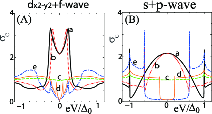
Figure 4: (Color online) Tunneling conductance $\sigma_{C}$ with $\beta=0.5$ and $Z=5$. A: $d_{x^{2}-y^{2}}+f$-wave and B: $s+p$-wave. a(solid line): $\Delta_{t}=\Delta_{0}$, $\Delta_{s}=0$, b(dotted line): $\Delta_{t}=0.8\Delta_{0}$, $\Delta_{s}=0.2\Delta_{0}$, c(dashed line): $\Delta_{t}=0.5\Delta_{0}$, $\Delta_{s}=0.5\Delta_{0}$, d(thin solid line): $\Delta_{t}=0.4\Delta_{0}$, $\Delta_{s}=0.6\Delta_{0}$, and e(dot-dashed line): $\Delta_{t}=0.2\Delta_{0}$, $\Delta_{s}=0.8\Delta_{0}$.

We also plot corresponding $\sigma_{C}$ for high ($Z=1$) and intermediate $(Z=2)$ transparent junctions. For $\Delta_{t}>\Delta_{s}$, $\sigma_{C}$ has a broad dip-like structure around $eV=0$ for $Z=1$, while it is slightly enhanced around $eV=0$ for $Z=2$ (curves $a$ and $b$ in Figs. 3(C) and (D)). On the other hand, for $\Delta_{s}>\Delta_{t}$, $\sigma_{C}$ always has a ZBCP (curves $d$ and $e$ in Figs.3(C) and (D)). The presence of TRI Majorana bound state gives a clear ZBCP with the increase of $Z$. As a reference, the tunneling conductance $\sigma_{C}$ for $d_{x^{2}-y^{2}}+f$-wave and $s+p$-wave cases are plotted in Fig. 4 for $Z=5$. ABS exists only for $\Delta_{s}<\Delta_{t}$. The $\sigma_{C}$ for $d_{x^{2}-y^{2}}+f$-wave has a ZBCP splitting reflecting the complex dispersion $\varepsilon_{b}$ shown in Fig. 4(A). On the other hand, for $s+p$-wave case, $\sigma_{C}$ has a broad ZBCP shown in Fig. 4(B). Summarizing Figs. 3 and 4, $\sigma_{C}$ for each paring state are qualitatively different from each other, which can be used to identify these pairings.

In conclusion, we have studied the ABS and resulting charge transport for $d_{xy}+p$-wave and $d_{x^{2}-y^{2}}+f$-wave superconductors. We find that the obtained dispersion of ABS in both cases have an anomalous structure. For $d_{xy}+p$-wave case, a novel TRI Majorana bound state is generated due to the spin-orbit coupling. The resulting charge conductance can serve as a guide to identify the TRI Majorana bound state and paring symmetry of NCS superconductors by tunneling spectroscopy.

This work is partly supported by the Sumitomo Foundation (M.S.) and the Grant-in-Aids for Scientific Research No. 22103005 (Y.T. and M.S.), No. 20654030 (Y.T.) and No.22540383 (M.S.).

References

(1) E. Bauer, ,
Phys. Rev. Lett. 92, 027003 (2004).
(2)
K. Togano et al., Phys. Rev. Lett. 93, 247004 (2004);
M. Nishiyama, ,
Phys. Rev. B
71, 220505(R) (2005).
(3) P. A. Frigeri, ,
Phys. Rev. Lett. 92, 097001 (2004).
(4) N. Reyren ., Science 317, 1196 (2007).
(5)L. P. Gor’kov and E. I. Rashba,
Phys. Rev. Lett. 87 037004 (2001).
(6)
S. Fujimoto, J. Phys. Soc. Jpn. 76, 051008 (2007).
(7) Y. Yanase and M. Sigrist, J. Phys. Soc. Jpn.
77, 124711 (2008);
Y. Tada, ,
New J. Phys.11, 055070 (2009).
(8)
J. Linder and A. Sudbø, Phys. Rev. B 76, 054511 (2007).
(9)
T. Yokoyama, ,
Phys. Rev. B 72 220504(R) (2005);
C. Iniotakis, ,
Phys. Rev. B 76, 012501 (2007);
M. Eschrig, , arXiv:1001.2486.
(10)
A.B. Vorontsov, , Phys. Rev. Lett.
101, 127003 (2008).
(11)
Y. Tanaka, ,
Phys. Rev. B 79, 060505(R) (2009).
(12)
M. Sato, Phys. Rev. B 73 214502 (2006);
M. Sato and S. Fujimoto, Phys. Rev. B 79, 094504 (2009).
(13)
C. K. Lu and S. Yip, Phys. Rev. B 80, 024504 (2009).
(14)
T. Yokoyama, ,
Phys. Rev. B 75, 172511 (2007);
T. Yokoyama, ,
J. Phys. Soc. Jpn. 77 064711 (2008).
(15)
K. Yada, ,
Phys. Rev. B 80 140509 (2009).
(16) L. J. Buchholtz and G. Zwicknagl, Phys. Rev. B 23,
5788 (1981);
C. R. Hu, Phys. Rev. Lett. 72, 1526 (1994).
(17)
Y. Tanaka and S. Kashiwaya, Phys.
Rev. Lett. 74, 3451 (1995);
S. Kashiwaya and Y. Tanaka, Rep. Prog. Phys. 63, 1641 (2000);
A. Biswas et al., Phys. Rev. Lett. 88, 207004 (2002);
B. Chesca et al., Phys. Rev. B 71, 104504 (2005), ,
73, 014529 (2006); 77, 184510 (2008);
M. Wagenknecht et al., Phys. Rev. Lett. 100, 227001 (2008).
(18) F. Wilczek, Nature Phys. 5, 614 (2009).
(19)
For example,
L. Fu and C. L. Kane, Phys. Rev. Lett. 100, 096407 (2008);
M. Sato, ,
Phys. Rev. Lett. 103, 020401 (2009);
Y. Tanaka, et. al.,
Phys. Rev. Lett. 103, 107002 (2009);
J. Linder, et. al., Phys. Rev. Lett. 104, 067001 (2010).
(20)
When the symmetry of the singlet component of pair potential
is -wave (-wave),
the number of the sign change of the real or imaginary part of
triplet one on the Fermi surface is two (six).
Thus, we call the mixed pair potential -wave (-wave).
(21)
A. P. Schnyder, et. al.,
Phys. Rev. B 78, 195125 (2008).
X.L. Qi, ,
Phys. Rev. Lett. 102, 187001 (2009);
R. Roy, arXiv:0803.2881;
M. Sato, Phys. Rev. B 79, 214526 (2009);
81, 220504(R) (2010).