Sensor Deployment for Network-like Environments

Abstract

This paper considers the problem of optimally deploying omnidirectional sensors, with potentially limited sensing radius, in a network-like environment. This model provides a compact and effective description of complex environments as well as a proper representation of road or river networks. We present a two-step procedure based on a discrete-time gradient ascent algorithm to find a local optimum for this problem. The first step performs a coarse optimization where sensors are allowed to move in the plane, to vary their sensing radius and to make use of a reduced model of the environment called collapsed network. It is made up of a finite discrete set of points, barycenters, produced by collapsing network edges. Sensors can be also clustered to reduce the complexity of this phase. The sensors’ positions found in the first step are then projected on the network and used in the second finer optimization, where sensors are constrained to move only on the network. The second step can be performed on-line, in a distributed fashion, by sensors moving in the real environment, and can make use of the full network as well as of the collapsed one. The adoption of a less constrained initial optimization has the merit of reducing the negative impact of the presence of a large number of local optima.

The effectiveness of the presented procedure is illustrated by a simulated deployment problem in an airport environment.

1 Introduction

Imagine a scenario where a toxic gas is spreading in an area or a building and safe paths have to be found to evacuate people. Or think of an airport environment where people moving through rooms and corridors has to be surveilled in order to detect and avoid terroristic actions. Or consider the need of measuring environmental quantities, such as temperature or humidity, on wide areas to the aim of improving theoretical models or making more accurate weather forecast.

There is a great number of situations that would greatly enjoy the use of network of sensors. Indeed, many of the previous tasks are difficult, or impossible, to be accomplished by a single sensor. The employment of a large number of sensors increases the robustness to sensor failure and communication disruption and make spatially-distributed observations possible. If sensors are able to move, the number of tasks they can perform is still greater.

Static and dynamic sensors’ networks need to be deployed in the environment, and the way this problem is solved can significantly affect the quality of service they have to provide.

1.1 Static Deployment and Locational Optimization

Sensors’ deployment problems are strictly related to facilities location-allocation problems, which are the subject of the locational optimization discipline ([9]).

In locational optimization objective functions are used to describe the interactions between users and facilities and among them. Users may find facilities desirable, hence they would like to exert an attractive force to facilities, or undesirable and they would repel them. The attractive model can describe allocation problems of useful services or facilities such as mailboxes, hospitals, fire stations, malls, etc. (see [9]). The repulsive one, instead, can be used to model problems where polluting or dangerous facilities (i.e. nuclear reactors, garbage dumps, etc.) are to be located far enough from urban conglomerations. An excellent survey on undesirable facility locations problems is given by [12] (see also [4]). These operational research problems can be converted in sensors’ deployment problems by considering sensors as facilities and points or areas, where events can happen or some quantities has to be measured, as users.

Two well known problems, involving one facility only, are the classical Weber and the obnoxious facility location problems (see [10, 8] for a recent heuristic solution). Three problems involving $p$ facilities are the $p$-center, $p$-median and $p$-dispersion problems. Some recent results on the $p$-center problem are in [29] and [5]. The latter paper addresses also the $p$-dispersion problem.

A classical $p$-median problem, close to the one considered in this paper, can be simply described as the one of finding the optimal location of $p$ facilities by minimizing the average distance of the demand points to the nearest facility (see [26] for a recent survey on heuristics methods to solve it). Close to the $p$-median problem is the multisource Weber problem, for which many heuristics exist ([2]). A more general formulation of these problems can be found in [7] and [11]. In [7] a dynamical (gradient descent) version of the Lloyd’s algorithm [23] has been presented to find a local optimum for a generalized $p$-median problem. A deterministic annealing optimization algorithm to solve the classical version is reported in [28]. The aforementioned solutions to the $p$-median problem, as well as many solutions to $p$-facilities problems, are based on the construction of a Voronoi Tesselation ([11, 27]).

1.2 Dynamic Deployment and Distributed Solutions

The use of moving, instead of static, sensor networks provide a great flexibility in solving sensing tasks, mainly when the environment is partially or completely unknown or is not directly accessible for safety reasons. In these cases, sensors are usually initially deployed randomly and hence need to move in order to acquire knowledge of the environment and to optimally re-deploy for their task. Furthermore, environments are usually not static and the network may experience sensor failure or loss. In these situations the properties of adaptivity and reconfigurability owned by a network of moving sensors turn out very useful.

A general tendency in robotic networks is to have sensors (agents) endowed with the same computational and sensing capabilities. This choice increases the overall robustness of the network, but usually calls for distributed coordination algorithms. Having equal sensors, indeed, naturally leads to define optimization and coordination algorithms based on local observations and local decisions ([13, 25, 18]). Many of the algorithms proposed in the previous section involve the solution of a global optimization problem requiring a complete knowledge of the environment and of sensors’ distribution. The solutions to $p$-center, $p$-dispersion and $p$-median problems proposed in [5, 7, 6], instead, are all spatially distributed, with the meaning that each sensor requires only the knowledge of positions of its neighbors (or even less if it has a limited sensing radius). This fact allows a distributed implementation where each sensor computes its next movement without centralized coordination.

Other solutions to the area-coverage problem look at sensors like particles subject to virtual forces or potential fields. The compositions of suitably defined attractive and repulsive forces is then used to make the network behaving in the desired fashion (spread sensors, avoid obstacles, keep connectivity, etc.). Representative for this kind of approach are the algorithms presented in [17, 33], or in [24], where also secure connectivity issues are considered. In [16], instead, it is raised the relevant problem of power consumption in wireless networks and three energy-efficient algorithms are presented for sensors’ deployment.

1.3 Network-like Environments and Paper Contributions

In this paper, we focus on network-like environments as there are surveillance or monitoring problems where such a kind of model can provide a more suitable description.

Network models represent a natural choice whenever environments have an intrinsic network structure. It is the case, for instance, when sensors have to be optimally deployed over a network of roads to monitor vehicular traffic, or in a river network to measure temperature or pollutants concentration. Even some location-allocation problems can involve networks. Consider, for instance, the case where useful facilities (i.e. schools, hospitals) have to be located in the interior of a network of roads, which is the source of a nuisance (i.e. noise, pollutants), with the goal of minimizing its harmful impact on them (see [8] for the case with one facility); or the dual problem of locating obnoxious facilities (i.e. dumps, industrial plants, mobile phone repeater antennas) reducing the hazard on the network.

Most notably, we think that a network-like model can provide an effective and compact description for complex environments, focusing only on major features and abstracting from those geometrical details which are less important for the deployment problem. The coverage of nonconvex environments with holes or obstacles, for instance, is a challenging task ([3]), which can enjoy significantly the use of a reduced network-like model. Environments with a complex structure, accounting for a large number of variously sized and shaped rooms, passages, forbidden areas and obstacles, can be reduced to a set of connected paths where the sensing task is more requested or where sensors are forced to pass. An airport is a very representative example of this kind of environments. In this case people moving throughout the airport can be aptly compared with a network flow and focus can be on paths more than on corridors, halls and lounges.

Many of the problems introduced in previous sections have been formulated even for a network-like environment ([30, 31]), but they usually consider a finite discrete set of demand points located on the network’s nodes and try to optimize the locations of facilities w.r.t. some objective function accounting for the distance from them. An important thread of works for the deployment of sensors both on plane and on a network is represented by the papers [19, 20, 21]. In such works, the authors propose powerful greedy algorithms that provide a constant approximation of the optimal solution. Their method, however, aims at solving a global static deployment problem, considering a finite set of demand points and allowing sensors to jump among positions.

In this paper, instead, we consider a deployment problem where sensors use local information to dynamically solve the optimization problem while they are moving in the environment. The constraints induced by the environment to the motion of sensors are explicitly considered. More precisely, we address a generalized $p$-median problem involving omnidirectional sensors with potentially limited sensing radius and we extend the formulation presented in [6, 7, 25] to network-like environments. The task is to find sensors’ positions that optimize an objective function defined on the network and accounting for the sensor’s features and preferential areas. This is a mixed problem, since the network is considered embedded in the plane (it is a continuous set of demand points) and the planar euclidean norm is used to measure the distance between sensors and network.

The core of the cited formulation and of our solution is a discrete-time gradient ascent algorithm based on Voronoi partitions and aiming at maximizing the objective function. It is a well known fact, however, that such a kind of algorithms can get stuck early in local optima, especially when sensors are forced to move in an over-constrained environment like a network. Moreover, the local maximum found by the algorithm is often greatly related to the initial sensors’ position.

For these reasons, we present a novel two-step procedure performing an initial coarse optimization, whose purpose is to provide a good starting point for a second finer optimization. The first step can be carried out off-line, either by a central unit, or by each sensor individually (without doing real movements). The impact of local optima is reduced by allowing sensors, in the initial optimization, to virtually move in $\mathbb{R}^{2}$ and to vary their sensing radius arbitrarily. In order to reduce the complexity of this phase, sensors can be initially clustered and the optimization problem solved for the clusters’ centers. After that, a desired number of sensors is spread close to clusters’ centers and the sensors’ positions thus found are projected on the closest edges of the network. The projected positions are then used in the second optimization, where sensors are constrained to move only on the network. The second step can be performed on-line, in a distributed fashion, by sensors moving in the real environment.

The use of a two-step procedure is motivated also by the very nature of some surveillance tasks, such as for instance airport surveillance, where a large number of individuals (sometimes referred to as mass objects [15]) are monitored. In these cases, sensors can solve the first step optimization using imprecise or estimated information and keeping still; then they can move to reach the final projected positions using planned routes compatible with the network. After this initial deployment, sensors can change their positions by dynamically solving a distributed optimization problem (second step) based on real measures taken from the (potentially varying) environment.

It is worth noting that the present procedure can be used to solve both static and dynamic deployment problems. Moreover, the first step deserves attention by its own, since it provides a solution to those problems involving facilities located in the interior of the network mentioned at the beginning of this section.

Another contribution of this paper is the introduction of a simplified model of the network (similar to the discretization in [14]) called collapsed network and consisting of finite many points. It is obtained by decomposing each segment of the original network in one or more sub-segments and collapsing each sub-segment in its barycenter. This model allows a coarser but faster optimization, since computations with barycenters are remarkably less than those needed by the full network. Collapsed network, hence, is intended mainly for fastening the first optimization, but can be used profitably also for the second step. Indeed, it turns out particularly useful in practical implementation involving hardware with limited computational capabilities.

As mentioned above, our work is related to that of [6, 7, 25]. In particular, the first step of the optimization, allowing sensors to move in $\mathbb{R}^{2}$, could be regarded as a specialization of the problem described in [7]. However, the different topology induced by the network introduces issues related to the explicit computation of the gradient and to the convergence of the maximization algorithm, which deserve special solutions. A relevant difference is that the gradient of the objective function presents discontinuity points caused by barycenters on the boundary edge of two neighboring Voronoi cells. Such barycenters can change allocation during sensors’ motion, inducing abrupt variations to the value of the objective function associated to each cell. This fact prevents a classical convergence proof for gradient algorithms, hence we consider our proof as a minor contribution of the paper. Some results about convergence may alternatively be derived by using the method of Kushner and Borkar ([22, 1]) of stochastic approximation to deal with our differential inclusion.

The outline of the paper is as follows. In section 2 the mathematical definitions of sensors, network and Voronoi covering are introduced along with the objective function to be maximized to solve the deployment problem. Section 3 is devoted to the introduction of the collapsed network and to the formulation, and proof of convergence, of a gradient ascent algorithm to solve the first step (subsection 3.1) and the second step (subsection 3.2) of the optimization procedure. Section 4 addresses the solution of the second step optimization involving the full network. Finally, a network describing an airport environment is used in section 5 to illustrate by simulations the effectiveness of the proposed optimization procedure. Conclusions and future research directions are reported in section 6.

2 Preliminaries and Problem Formulation

In this section we introduce the mathematical framework to describe the sensors, the network and its Voronoi covering.

Definition 1

Given two points $p_{1},p_{2}\in\mathbb{R}^{2}$, with $p_{1}\neq p_{2}$, $s_{12}=[p_{1},p_{2}]\subset\mathbb{R}^{2}$ is the segment joining $p_{1}$ and $p_{2}$ and $s_{12}^{o}=(p_{1},p_{2})$ is the open segment between them. We define length of a segment $s_{12}$ as $\ell(s_{12})=\left\|p_{2}-p_{1}\right\|$, where $\left\|\cdot\right\|$ is the Euclidean norm; barycenter of a segment $s_{12}$ the point $b(s_{12})=\frac{1}{2}\left(p_{2}+p_{1}\right)\in$ $s_{12}$; partition of a segment $s=[p_{1},p_{2}]$ in $k$ sub-segments, the set of segments $\left\{s_{i}\right\}_{i=1,\ldots,k}$ given by

$$s_{i}=\left[p_{1}+\left(i-1\right)\frac{\left(p_{2}-p_{1}\right)}{k},p_{1}+i\frac{\left(p_{2}-p_{1}\right)}{k}\right]\text{.}$$

Definition 2

A network $\mathcal{N}=(\mathcal{V},\mathcal{S})$ is a subset of $\mathbb{R}^{2}$ consisting of a set of points $\mathcal{V}=\left\{v_{1},\ldots,v_{n}\in\mathbb{R}^{2},~{}v_{i}\neq v_{j}~{}\forall i\neq j\right\}$ and a set of segments $\mathcal{S}\subseteq\{s_{ij}=[v_{i},v_{j}]\subset\mathbb{R}^{2},~{}i,j\in\left\{1,\ldots,n\right\}~{}i\neq j\}$, such that:

i)

$\forall v_{i}\in\mathcal{V}$, $\exists v_{j}\in\mathcal{V}$, $v_{i}\neq v_{j}$ such that $s_{ij}\in\mathcal{S}$ (no isolated vertex);

ii)

$\forall i,j,h,k\in\left\{1,\ldots,n\right\},$ $(i,j)\neq(h,k),$ $s_{ij}^{o}\cap s_{hk}^{o}=\emptyset$ (no segment intersection).

Definition 3

Given a network $\mathcal{N}$ and a set of points $\mathcal{P}=\left\{p_{1},\ldots,p_{m}\right\}\subset\mathcal{N}$, the Voronoi covering of $\mathcal{N}$ generated by $\mathcal{P}$ with respect to the Euclidean norm is the collection of sets $\left\{V_{i}^{\mathcal{N}}(\mathcal{P})\right\}_{i\in\left\{1,\ldots,m\right\}}$ defined by

$$V_{i}^{\mathcal{N}}(\mathcal{P})=\left\{q\in\mathcal{N}\mid\left\|q-p_{i}\right\|\leq\left\|q-p_{j}\right\|,\text{~{}}\forall p_{j}\in\mathcal{P}\right\}\text{.}$$

Remark 4

It is straightforward to recognize that $V_{i}^{\mathcal{N}}(\mathcal{P})$ can be equivalently defined as $V_{i}^{\mathcal{N}}(\mathcal{P})=V_{i}(\mathcal{P})\cap\mathcal{N}$, where $V_{i}(\mathcal{P})$ is the $i$-th cell of the usual Voronoi partition of $\mathbb{R}^{2}$ generated by $\mathcal{P}$. The previous definition is about a covering and not a partition since neighboring cells can have a nontrivial intersection: a portion of a segment can belong to the shared edge of two cells $V_{i}(\mathcal{P})$ and $V_{j}(\mathcal{P})$.

We adapt the framework provided in [6] to describe the sensors’ and network features. Each sensor is modeled by the (same) performance function $f:\mathbb{R}_{+}\rightarrow\mathbb{R}$, that is a non-increasing and piecewise differentiable map having a finite number of bounded discontinuities at $R_{1},\ldots,R_{N}\in\mathbb{R}_{+}$, with $R_{1}<\ldots<R_{N}$. We can set $R_{0}=0$, $R_{N+1}=+\infty$ and write

$$f(x)=\sum_{\alpha=1}^{N+1}f_{\alpha}(x)1_{[R_{\alpha-1},R_{\alpha})}(x)\text{,}$$ (1)

with $f_{\alpha}:[R_{\alpha-1},R_{\alpha}]\rightarrow\mathbb{R}$, $\alpha\in\{1,\ldots,N+1\}$ non-increasing continuously differentiable functions such that $f_{\alpha}(R_{\alpha})>f_{\alpha+1}(R_{\alpha})$ for $\alpha\in\{1,\ldots,N\}$. In order to model regions of the network with different importance, we can use a density function $\phi:\mathcal{N}\rightarrow\mathbb{R}_{+}$, which is bounded and measurable on $\mathcal{N}$. Given $g:\mathbb{R}^{2}\rightarrow\mathbb{R}$ we indicate by ${\displaystyle\int\nolimits_{\mathcal{N}}}g(q)dq$ (respectively ${\displaystyle\int\nolimits_{V_{i}^{\mathcal{N}}(\mathcal{P})}}g(q)dq$) the sum of the linear integrals of $g$ over the segments of $\mathcal{N}$ (respectively $V_{i}^{\mathcal{N}}(\mathcal{P})$) using an arc-length parameterization. With these functions we can define the multi-center function $\mathcal{H}:\mathcal{N}^{m}\rightarrow\mathbb{R}$ for $m$ sensors located in $\mathcal{P}=\left\{p_{1},\ldots,p_{m}\right\}\subset\mathcal{N}$

$$\mathcal{H}\left(\mathcal{P}\right)={\displaystyle\int\nolimits_{\mathcal{N}}}\max_{i\in\left\{1,\ldots,m\right\}}f\left(\left\|q-p_{i}\right\|\right)\phi\left(q\right)dq\text{.}$$ (2)

We can also provide an alternative expression for (2) based on the Voronoi covering induced by $\mathcal{P}$ as follows

$$\mathcal{H}(\mathcal{P})={\displaystyle\sum\limits_{i=1}^{m}}{\displaystyle\int\nolimits_{V_{i}^{\mathcal{N}}(\mathcal{P})}}f\left(\left\|q-p_{i}\right\|\right)\phi\left(q\right)dq-{\displaystyle\sum\limits_{\Delta_{hk}^{\mathcal{N}}\in\Delta^{\mathcal{N}}}}{\displaystyle\int\nolimits_{\Delta_{hk}^{\mathcal{N}}}}f\left(\left\|q-p_{h}\right\|\right)\phi\left(q\right)dq\text{,}$$ (3)

where $\Delta_{hk}^{\mathcal{N}}\triangleq V_{h}^{\mathcal{N}}(\mathcal{P})\cap V_{k}^{\mathcal{N}}(\mathcal{P})$ and $\Delta^{\mathcal{N}}\triangleq\left\{\Delta_{hk}^{\mathcal{N}}\mid h<k,~{}\forall h,k\in\left\{1,\ldots,m\right\}\right\}$. The second term in (3) is not null if and only if there exists a non trivial segment $s\subseteq s_{ij}\in\mathcal{S}$ such that $s\subset\Delta_{hk}^{\mathcal{N}}$ for some $i,j\in\left\{1,\ldots,n\right\}$ and $h,k\in\left\{1,\ldots,m\right\}$.

3 Deployment over a Collapsed Network

In a collapsed network each segment of the original network is decomposed in one or more sub-segments and each sub-segment is collapsed in its barycenter. Chosen a value for $r$ guaranteeing a good approximation, we can build the $r$-collapsed network $\mathcal{C}_{r}^{\mathcal{N}}$ as follows:

Definition 5 ($r$-Collapsed Network)

Given a network $\mathcal{N}=(\mathcal{V},\mathcal{S})$ and $r>0$, $\forall s\in\mathcal{S}$ consider its partition in $k_{s}=\left\lceil\frac{\ell(s)}{r}\right\rceil$ sub-segments $s_{i}$ (having at most length $r$) and the associated set of barycenters $\left\{b\left(s_{i}\right)\right\}_{i=1,\ldots,k_{s}}$. We define the $r$-collapsed network associated to $\mathcal{N}$ the set of points $\mathcal{C}_{r}^{\mathcal{N}}={\displaystyle\bigcup\nolimits_{s\in\mathcal{S}}}\left\{b\left(s_{i}\right)\right\}_{i=1,\ldots,k_{s}}$.

The multi-center function must be re-defined since the integration domain is now a discrete set represented by the barycenters. Hence we set

$$\mathcal{H}(\mathcal{P})={\displaystyle\sum\limits_{b_{e}\in\mathcal{C}_{r}^{\mathcal{N}}}}\max_{i\in\left\{1,\ldots,m\right\}}f\left(\left\|b_{e}-p_{i}\right\|\right)\phi_{b_{e}}\text{,}$$ (4)

where $\phi_{b_{e}}$ are suitable (density) weights assigned to barycenters.

3.1 Sensors Moving in $\mathbb{R}^{2}$

In this section we solve the deployment problem for a collapsed network and sensors moving in $\mathbb{R}^{2}$, which constitutes the first step of our optimization procedure.

Also for the multi-center function (4) we can provide an alternative expression using the Voronoi covering. We need the following definition:

Definition 6

Given an $r$-collapsed network $\mathcal{C}_{r}^{\mathcal{N}}$ for some $r\in\mathbb{R}_{+}$ and a set of points $\mathcal{P}=\left\{p_{1},\ldots,p_{m}\right\}\subset\mathbb{R}^{2}$, the Voronoi covering of $\mathcal{C}_{r}^{\mathcal{N}}$ generated by $\mathcal{P}$ with respect to the Euclidean norm is the collection of sets $\left\{V_{i}^{\mathcal{C}_{r}^{\mathcal{N}}}(\mathcal{P})\right\}_{i\in\left\{1,\ldots,m\right\}}$ defined by

$$V_{i}^{\mathcal{C}_{r}^{\mathcal{N}}}(\mathcal{P})=\left\{b\in\mathcal{C}_{r}^{\mathcal{N}}\mid\left\|b-p_{i}\right\|\leq\left\|b-p_{j}\right\|,\text{~{}}\forall p_{j}\in\mathcal{P}\right\}\text{.}$$

We define also the boundary of a Voronoi cell as

$$\partial V_{i}^{\mathcal{C}_{r}^{\mathcal{N}}}(\mathcal{P})=\left\{b\in\mathcal{C}_{r}^{\mathcal{N}}\mid\left\|b-p_{i}\right\|=\left\|b-p_{j}\right\|,\text{~{}}\forall p_{j}\in\mathcal{P}\right\}\text{,}$$

and, in order to simplify the problem, we make the following assumption

Assumption 7

$\partial V_{i}^{\mathcal{C}_{r}^{\mathcal{N}}}(\mathcal{P})=\emptyset$ $\forall i\in\left\{1,\ldots,m\right\}$.

With this assumption the multi-center function (4) can be written also as

$$\mathcal{H}(\mathcal{P})={\displaystyle\sum\limits_{i=1}^{m}}{\displaystyle\sum\limits_{b_{e}\in V_{i}^{\mathcal{C}_{r}^{\mathcal{N}}}(\mathcal{P})}}f\left(\left\|b_{e}-p_{i}\right\|\right)\phi_{b_{e}}\text{,}$$ (5)

or, setting $\mathrm{dist}(q,\mathcal{P})=\min_{i\in\left\{1,\ldots,m\right\}}\left\|q-p_{i}\right\|$, as

$$\mathcal{H}(\mathcal{P})={\displaystyle\sum\limits_{b_{e}\in\mathcal{C}_{r}^{\mathcal{N}}}}f\left(\mathrm{dist}(b_{e},\mathcal{P})\right)\phi_{b_{e}}\text{.}$$ (6)

Remark 8

$\mathcal{H}(\mathcal{P})$ is not globally Lipschitz as $f(\cdot)$ is not a continuous function. However, if $f(x)$ is continuous and piecewise differentiable with bounded derivative, then $\mathcal{H}(\mathcal{P})$ is globally Lipschitz. In order to prove the global Lipschitz continuity, let us consider two sets of points $\mathcal{P}=\left\{p_{1},\ldots,p_{m}\right\}\subset\mathbb{R}^{2}$ and $\mathcal{P}^{\prime}=\left\{p_{1}^{\prime},\ldots,p_{m}^{\prime}\right\}\subset\mathbb{R}^{2}$ and compute

$$\mathcal{H}(\mathcal{P})-\mathcal{H}(\mathcal{P}^{\prime}) ={\displaystyle\sum\limits_{b_{e}\in\mathcal{C}_{r}^{\mathcal{N}}}}\left[f\left(\mathrm{dist}(b_{e},\mathcal{P})\right)-f\left(\mathrm{dist}(b_{e},\mathcal{P}^{\prime})\right)\right]\phi_{b_{e}}$$

$$\leq{\displaystyle\sum\limits_{b_{e}\in\mathcal{C}_{r}^{\mathcal{N}}}}\left\|\frac{\partial f}{\partial x}\right\|_{\infty}\left|\mathrm{dist}(b_{e},\mathcal{P})-\mathrm{dist}(b_{e},\mathcal{P}^{\prime})\right|\phi_{b_{e}}$$

$$\leq\left({\displaystyle\sum\limits_{b_{e}\in\mathcal{C}_{r}^{\mathcal{N}}}}\phi_{b_{e}}\right)\left\|\frac{\partial f}{\partial x}\right\|_{\infty}\left\|\mathcal{P}-\mathcal{P}^{\prime}\right\|\text{,}$$

where $\left\|\frac{\partial f}{\partial x}\right\|_{\infty}$ is the $L_{\infty}$-norm of $\frac{\partial f}{\partial x}$.

Theorem 9

The multi-center function $\mathcal{H}$ is continuously differentiable on $\left(\mathbb{R}^{2}\right)^{m}\setminus\left(\mathcal{D}_{\mathcal{C}_{r}^{\mathcal{N}}}\right)^{m}$, where

$$\mathcal{D}_{\mathcal{C}_{r}^{\mathcal{N}}}\triangleq{\displaystyle\bigcup\nolimits_{b_{e}\in\mathcal{C}_{r}^{\mathcal{N}}}}\left\{q\in\mathbb{R}^{2}\mid\left\|b_{e}-q\right\|=R_{i},~{}\forall i=1,\ldots,N\right\}$$

is the discontinuity set of $f(\cdot)$ in $\mathbb{R}^{2}$. Moreover, for each $h\in\left\{1,\ldots,m\right\}$

$$\frac{\partial\mathcal{H}(\mathcal{P})}{\partial p_{h}}={\displaystyle\sum\limits_{b_{e}\in V_{h}^{\mathcal{C}_{r}^{\mathcal{N}}}(\mathcal{P})}}\frac{\partial}{\partial p_{h}}f\left(\left\|b_{e}-p_{h}\right\|\right)\phi_{b_{e}}\text{.}$$ (7)

Proof. The continuous differentiability of $\mathcal{H}$ on $\left(\mathbb{R}^{2}\right)^{m}\setminus$ $\left(\mathcal{D}_{\mathcal{C}_{r}^{\mathcal{N}}}\right)^{m}$ is a straight consequence of the same property of $f(\cdot)$ on $\mathbb{R}^{2}\setminus$ $\mathcal{D}_{\mathcal{C}_{r}^{\mathcal{N}}}$. As concerns the gradient, using (6) we have

$$\frac{\partial\mathcal{H}(\mathcal{P})}{\partial p_{h}} =\frac{\partial}{\partial p_{h}}{\displaystyle\sum\limits_{b_{e}\in\mathcal{C}_{r}^{\mathcal{N}}}}f\left(\mathrm{dist}(b_{e},\mathcal{P})\right)\phi_{b_{e}}$$

$$={\displaystyle\sum\limits_{b_{e}\in\mathcal{C}_{r}^{\mathcal{N}}}}\frac{\partial}{\partial p_{h}}f\left(\mathrm{dist}(b_{e},\mathcal{P})\right)\phi_{b_{e}}\text{.}$$

In the hypothesis of Assumption 7, we have that the index set $I_{be}=\operatorname*{argmin}_{i\in\left\{1,\ldots,m\right\}}\left(\left\|b_{e}-p_{i}\right\|\right)$ has cardinality $1$. Hence, $\forall b_{e}$ such that $I_{be}\equiv i\neq h$, $\frac{\partial}{\partial p_{h}}f\left(\mathrm{dist}(b_{e},\mathcal{P})\right)=0$ and

$$\frac{\partial\mathcal{H}(\mathcal{P})}{\partial p_{h}}={\displaystyle\sum\limits_{\left\{b_{e}\in\mathcal{C}_{r}^{\mathcal{N}}\mid I_{be}\equiv h\right\}}}\frac{\partial}{\partial p_{h}}f\left(\left\|b_{e}-p_{h}\right\|\right)\phi_{b_{e}}\text{,}$$

whereby the thesis follows using the definition of $V_{h}^{\mathcal{C}_{r}^{\mathcal{N}}}(\mathcal{P})$.   

The sensors’ location-allocation problem can be addressed by means of a gradient-like algorithm. If a continuous time implementation is looked for, the following fictitious dynamics would be associated to the sensors’ positions

$$\mathcal{\dot{P}}=\nabla\mathcal{H(P)}\text{.}$$ (8)

Unfortunately, this dynamics conveys some problems. It is well defined as long as Assumption 7 and Theorem 9 are fulfilled, but these hypotheses are, in fact, too stringent for the algorithm to work properly. Indeed, they would require the evolution of the sensors to avoid any position in the discontinuity set and the barycenters not to enter or exit the Voronoi cells where they are at the initial time instant.

First of all we can reduce the analysis to continuously differentiable functions to avoid issues related to the existence of the gradient. Still the relaxation of Assumption 7 induces some problems on the definition of the gradient. Barycenters on a boundary edge of a Voronoi cell belong to all the cells sharing that edge. All sensors’ positions producing these configurations are discontinuity points for $\nabla\mathcal{H(P)}$. Roughly speaking, the gradient takes different values depending on which cell the shared barycenters are assumed to belong to. This fact makes the equation (8) a set of differential equations with discontinuous right-hand side.

The problem of shared barycenters can be solved by adding a lexicographic criterion to the definitions based on the euclidean distance. Indeed, with this criterion barycenters on boundary edges are allocated univocally to the sensor having the lower index (w.r.t. the Lexicographic Order (L.O.)) among sharing sensors. This fact allows us to define a genuine Voronoi partition, no longer a covering, whose generic cell is given by (compare with Definition 6):

$$V_{i}^{\mathcal{C}_{r}^{\mathcal{N}}}(\mathcal{P})=\{b\in\mathcal{C}_{r}^{\mathcal{N}}\mid\left\|b-p_{i}\right\|\leq\left\|b-p_{j}\right\|~{}\forall p_{j}\in\mathcal{P}~{}\wedge\text{~{}}\\ \left\|b-p_{i}\right\|<\left\|b-p_{j}\right\|\text{ if }j<i\text{ w.r.t. the L.O.}\mathcal{\}}\text{.}$$ (9)

We must now define a generalized (lexicographic) gradient of $\mathcal{H}$, $\nabla_{l}\mathcal{H(P)}$, according to this new definition. $\forall b_{e}\in V_{i}^{\mathcal{C}_{r}^{\mathcal{N}}}(\mathcal{P})\setminus\partial V_{i}^{\mathcal{C}_{r}^{\mathcal{N}}}(\mathcal{P})$ we use the classical formula given by (7). $\forall b_{e}\in\partial V_{i}^{\mathcal{C}_{r}^{\mathcal{N}}}(\mathcal{P})$ notice that the partial derivative of $f$, $\frac{\partial}{\partial p_{h}}f\left(\left\|b_{e}-p_{h}\right\|\right)$, exists and is well defined. In the light of this remark we can write the $h$-th component of the generalized (lexicographic) gradient of $\mathcal{H}$ as

$$\frac{\partial_{l}\mathcal{H}(\mathcal{P})}{\partial p_{h}}\triangleq{\displaystyle\sum\limits_{b_{e}\in V_{h}^{\mathcal{C}_{r}^{\mathcal{N}}}(\mathcal{P})}}\frac{\partial}{\partial p_{h}}f\left(\left\|b_{e}-p_{h}\right\|\right)\phi_{b_{e}}\text{,}$$ (10)

which is formally equal to the formula (7) provided by Theorem 9.

The differential equation using this new definition for the gradient, however, does not imply the existence and uniqueness of the solution, and this proof may turn out to be complex due to special sensors’ and barycenters’ configurations. Moreover, the formula (10) accounts only for the infinitesimal perturbations of sensors’ position not inducing any barycenters to enter or exit Voronoi cells, hence changing their allocation.

In order to simplify the convergence proof and to provide an algorithm which is more suitable for a realistic implementation, we consider here a discrete-time version of the gradient algorithm. In our case, the discrete-time implementation can overcome the problems with discontinuity gradients due to the properties of the function $\mathcal{H}$ and its discontinuity points, as it is shown by the following theorem.

Theorem 10

Consider the following discrete-time evolution for the sensors’ positions

$$\mathcal{P}^{(k+1)}=\mathcal{P}^{(k)}+\delta_{k}\nabla_{l}\mathcal{H}(\mathcal{P}^{(k)})\text{,}$$ (11)

where the $h$-th component of $\nabla_{l}\mathcal{H}$ is given by (10) and $\mathcal{H}:\mathbb{R}^{2m}\rightarrow\mathbb{R}$ as in (5). If $f(\cdot)$ has locally bounded second derivatives, then, for suitable $\delta_{k}$, $\mathcal{P}^{(k)}$ lies in a bounded set and

i)

$\mathcal{H}(\mathcal{P}^{(k)})$ is monotonically nondecreasing;

ii)

$\mathcal{P}^{(k)}$ converges to the set of critical points of $\mathcal{H}$.

Proof. It is easy to see that there exists a ball $B\supseteq\mathcal{N}$ such that, if $p_{i}\in\partial B$, then $\frac{\partial_{l}\mathcal{H}(\mathcal{P})}{\partial p_{i}}$ points inside $B$. Thus the fact that $\mathcal{P}^{(k)}$ is bounded for $\delta_{k}$ sufficiently small, easily follows. According to the definition in equation (9) of a Voronoi cell using the lexicographic rule, we can define

$$\mathcal{H}_{p_{i}}(\mathcal{P})={\displaystyle\sum\limits_{b_{e}\in V_{i}^{\mathcal{C}_{r}^{\mathcal{N}}}(\mathcal{P})}}f\left(\left\|b_{e}-p_{i}\right\|\right)\phi_{b_{e}}\text{,}$$

hence we can write $\mathcal{H}(\mathcal{P})={\displaystyle\sum\limits_{i=1}^{m}}\mathcal{H}_{p_{i}}(\mathcal{P})$. We must prove that $\mathcal{H}_{p_{i}}(\mathcal{P}^{(k+1)})\geq\mathcal{H}_{p_{i}}(\mathcal{P}^{(k)})$ for $\forall p_{i}\in\mathcal{P}^{(k)}$ obeying the discrete-time evolution (11) and that $\exists p_{i}\in\mathcal{P}^{(k)}$ such that $\mathcal{H}_{p_{i}}(\mathcal{P}^{(k+1)})>\mathcal{H}_{p_{i}}(\mathcal{P}^{(k)})$ if $\mathcal{P}^{(k)}$ does not belong to the set of critical points of $\mathcal{H}$. Define $\mathcal{H}_{p_{i}}^{u}(\mathcal{P}^{(k+1)})={\displaystyle\sum\limits_{b_{e}\in V_{i}^{\mathcal{C}_{r}^{\mathcal{N}}}(\mathcal{P}^{(k)})}}f\left(\left\|b_{e}-p_{i}^{(k+1)}\right\|\right)\phi_{b_{e}}$, that is the cost $\mathcal{H}_{p_{i}}(\mathcal{\cdot})$ computed by using the new sensors’ positions $\mathcal{P}^{(k+1)}$ but the old allocation of barycenters to sensors, i.e. the Voronoi partition generated by $\mathcal{P}^{(k)}$. Therefore, we write

$$\mathcal{H}_{p_{i}}^{u}(\mathcal{P}^{(k+1)}) =\mathcal{H}_{p_{i}}(\mathcal{P}^{(k)}+\delta_{k}^{i}\nabla_{l}\mathcal{H}(\mathcal{P}^{(k)}))$$

$$=\mathcal{H}_{p_{i}}(\mathcal{P}^{(k)})+\delta_{k}^{i}\left(\frac{\partial\mathcal{H}_{p_{i}}(\mathcal{P}^{(k)})}{\partial p_{i}}\cdot\left(\nabla_{l}\mathcal{H}(\mathcal{P}^{(k)})\right)_{i}\right)+o\left((\delta_{k}^{i})^{2}\right)$$

$$=\mathcal{H}_{p_{i}}(\mathcal{P}^{(k)})+\delta_{k}^{i}\left\|\frac{\partial\mathcal{H}_{p_{i}}(\mathcal{P}^{(k)})}{\partial p_{i}}\right\|^{2}+o\left((\delta_{k}^{i})^{2}\right)\text{,}$$ (12)

where the (generalized) gradient is computed by means of the lexicographic assignment based on the Voronoi partition generated by $\mathcal{P}^{(k)}$. If the Voronoi partitions generated by $\mathcal{P}^{(k+1)}$ and $\mathcal{P}^{(k)}$ coincide (same barycenters’ allocation), then $\mathcal{H}_{p_{i}}(\mathcal{P}^{(k+1)})=\mathcal{H}_{p_{i}}^{u}(\mathcal{P}^{(k+1)})$ and we can assert directly that $\mathcal{H}_{p_{i}}(\mathcal{P}^{(k+1)})\geq\mathcal{H}_{p_{i}}(\mathcal{P}^{(k)})$ or $\mathcal{H}_{p_{i}}(\mathcal{P}^{(k+1)})>\mathcal{H}_{p_{i}}(\mathcal{P}^{(k)})$ if $\frac{\partial\mathcal{H}_{p_{i}}(\mathcal{P}^{(k)})}{\partial p_{i}}\neq 0$, that is if $\mathcal{P}^{(k)}$ does not belong to the set of critical points of $\mathcal{H}$. It is worth noting that similar remarks about the strict inequality apply also in what follows and they will not be repeated. If the barycenters’ allocation is different, $\mathcal{H}_{p_{i}}(\mathcal{P}^{(k+1)})$ may be smaller than $\mathcal{H}_{p_{i}}^{u}(\mathcal{P}^{(k+1)})$ and we cannot say anything about its relation with $\mathcal{H}_{p_{i}}(\mathcal{P}^{(k)})$. This fact is due to the presence of barycenters changing allocation during the sensors’ evolution, hence the cells involved in the change cannot be considered independently. Let us consider for simplicity only one barycenter $b_{e}\in V_{j}^{\mathcal{C}_{r}^{\mathcal{N}}}(\mathcal{P}^{(k)})$ and suppose that at step $k+1$ $b_{e}\in V_{i}^{\mathcal{C}_{r}^{\mathcal{N}}}(\mathcal{P}^{(k+1)})$. With this assumption no barycenters can enter or exit the union of the two cells but $b_{e}$. We have

$$\mathcal{H}_{p_{i}}(\mathcal{P}^{(k+1)}) =\mathcal{H}_{p_{i}}^{u}(\mathcal{P}^{(k+1)})+f\left(\left\|b_{e}-p_{i}^{(k+1)}\right\|\right)\phi_{b_{e}}$$

$$\mathcal{H}_{p_{j}}(\mathcal{P}^{(k+1)}) =\mathcal{H}_{p_{j}}^{u}(\mathcal{P}^{(k+1)})-f\left(\left\|b_{e}-p_{j}^{(k+1)}\right\|\right)\phi_{b_{e}}\text{.}$$ (13)

In other words, $\mathcal{H}_{p_{i}}(\mathcal{P}^{(k+1)})$ is grown w.r.t. the ideal value $\mathcal{H}_{p_{i}}^{u}(\mathcal{P}^{(k+1)})$ due to the allocation of $b_{e}$ to $p_{i}^{(k+1)}$, whereas, $\mathcal{H}_{p_{j}}(\mathcal{P}^{(k+1)})$ is decreased w.r.t. $\mathcal{H}_{p_{i}}^{u}(\mathcal{P}^{(k+1)})$ by the contribution that $b_{e}$ would have given if it were allocated to $p_{j}^{(k+1)}$ even at the step $k+1$. It is worth noting that if $b_{e}$ changes allocation from $p_{j}^{(k+1)}$ to $p_{i}^{(k+1)}$, then $\left\|b_{e}-p_{i}^{(k+1)}\right\|\leq\left\|b_{e}-p_{j}^{(k+1)}\right\|$ (the equality holds only if $b_{e}\in\partial V_{i}^{\mathcal{C}_{r}^{\mathcal{N}}}(\mathcal{P}^{(k+1)})\cap\partial V_{j}^{\mathcal{C}_{r}^{\mathcal{N}}}(\mathcal{P}^{(k+1)})$ and, being $i<j$, the allocation is induced by the lexicographic rule). Therefore, due to the monotonicity of $f$, $f\left(\left\|b_{e}-p_{i}^{(k+1)}\right\|\right)\geq f\left(\left\|b_{e}-p_{j}^{(k+1)}\right\|\right)$. Summing up, we have

$$\mathcal{H}_{p_{i}}(\mathcal{P}^{(k+1)})+\mathcal{H}_{p_{j}}(\mathcal{P}^{(k+1)}) \geq\mathcal{H}_{p_{i}}^{u}(\mathcal{P}^{(k+1)})+\mathcal{H}_{p_{j}}^{u}(\mathcal{P}^{(k+1)})$$

$$=\mathcal{H}_{p_{i}}(\mathcal{P}^{(k)})+\delta_{k}^{i}\left\|\frac{\partial\mathcal{H}_{p_{i}}(\mathcal{P}^{(k)})}{\partial p_{i}}\right\|^{2}+o\left((\delta_{k}^{i})^{2}\right)$$

$$+\mathcal{H}_{p_{j}}(\mathcal{P}^{(k)})+\delta_{k}^{j}\left\|\frac{\partial\mathcal{H}_{p_{j}}(\mathcal{P}^{(k)})}{\partial p_{j}}\right\|^{2}+o\left((\delta_{k}^{j})^{2}\right)\text{.}$$

There exist some constants $c_{k}^{ij},\delta_{k}^{ij}>0$ such that

$$\mathcal{H}_{p_{i}}(\mathcal{P}^{(k+1)})+\mathcal{H}_{p_{j}}(\mathcal{P}^{(k+1)})\geq\mathcal{H}_{p_{i}}(\mathcal{P}^{(k)})+\mathcal{H}_{p_{j}}(\mathcal{P}^{(k)})+\delta_{k}^{ij}c_{k}^{ij}+o\left((\delta_{k}^{ij})^{2}\right)\text{.}$$

Extending the same reasoning to more complex configurations involving more than one common boundary edge and more than two neighboring cells, we can say that $\exists c_{k},\delta_{k}>0$ such that

$$\mathcal{H}(\mathcal{P}^{(k+1)})={\displaystyle\sum\limits_{i=1}^{m}}\mathcal{H}_{p_{i}}(\mathcal{P}^{(k+1)})\geq\mathcal{H}(\mathcal{P}^{(k)})+\delta_{k}c_{k}+o(\delta_{k}^{2})\text{.}$$

This proves assertion i). Assertion ii) can be proved by exploiting the results of Section 3.2 of [6]. More precisely, using the fact that $\mathcal{P}^{(k)}$ is bounded and $f$ has locally bounded second derivatives, then there exists $\bar{\delta}>0$ such that we can choose $\delta_{k}\geq\bar{\delta}$. Then we conclude, using Proposition 3.4 of [6], that assertion ii) is true.   

Remark 11 (Distributed Implementation)

The use of a gradient ascent algorithm based on a Voronoi partition, allows us to solve not only a static deployment problem, but also a dynamic one. As shown in [6], this kind of algorithms is spatially distributed, with the meaning that the $i$-th sensor needs only to know the position of its neighbors in order to determine the boundary of its cell and, hence, to compute $\frac{\partial\mathcal{H}_{p_{i}}}{\partial p_{i}}$. For the same reason the $i$-th sensor can choose the value of the step-size $\delta_{k}^{i}$ independently of the other sensors simply performing locally a classical line search algorithm. This property makes the algorithm suitable for a spatially distributed implementation.

The independence in the choice of the step-sizes $\delta_{k}^{i}$ is obviously preserved in each period $k$, as long as a synchronous implementation is considered. In this case sensors have access to a global clock, or perform a synchronization algorithm. At the beginning of the the $k$-th period (instant $t_{k}$), all sensors are idle, build their Voronoi cells and compute their gradients and step-sizes, then they move until, at most, the end of the period (instant $t_{k+1}$). If, instead, an asynchronous implementation is considered, further hypotheses are necessary to ensure that independence is preserved. Unfortunately, the discontinuity of the gradient prevent us from using the results of [32]. But, if a sensor has the capability to detect when its neighbors start and stop moving and when a new sensor joins the neighborhood, the asynchronous algorithm presented in [7] (Table IV), can be applied, thus automatically recovering the independence.

Remark 12

In the previous theorem, for sake of simplicity, we did not consider degenerate configurations where different sensors have the same position ($p_{i}=p_{j}$ for $i\neq j$). But it can be proved that if the initial positions of sensors are not degenerate, sensors can always choose a suitable $\delta_{k}^{i}$ to avoid the occurrence of these configurations.

3.2 Sensors Moving on the Network

This section is devoted to the case of sensors constrained to move on the network and sensing a collapsed network. Therefore, these results are suitable for an implementation of the second step of our procedure on hardware with limited computational capabilities.

We still assume $f(\cdot)$ to be a continuously differentiable function and we make use of the lexicographic criterion for the barycenter allocation. As concerns sensors’ motion, however, we cannot use directly the gradient since the sensors have to remain on the network. We must consider now the directional derivative of $\mathcal{H}$ along the edges of the network.

Following the guidelines of the previous section, the following theorem can be proved.

Theorem 13

Given a network $\mathcal{N}=(\mathcal{V},\mathcal{S})$ and the related $r$-collapsed network $\mathcal{C}_{r}^{\mathcal{N}}$, the multi-center function $\mathcal{H}$ is continuously differentiable almost everywhere on $\mathcal{N}^{m}$. In particular, on each open segment $s_{ij}^{o}$ such that $s_{ij}\in\mathcal{S}$, given the unit vector $w_{ij}$ such that $s_{ij}\cdot w_{ij}=\left\|s_{ij}\right\|$, the directional derivative in $p_{h}\in s_{ij}^{o}$ along $w_{ij}$ is

$$D_{w_{ij}}\mathcal{H(P)}[p_{h}] =\left(\frac{\partial_{l}\mathcal{H}}{\partial p_{h}}(\mathcal{P})\cdot w_{ij}\right)w_{ij}$$ (14)

$$\frac{\partial_{l}\mathcal{H}}{\partial p_{h}}(\mathcal{P}) ={\displaystyle\sum\limits_{b_{e}\in V_{h}^{\mathcal{C}_{r}^{\mathcal{N}}}(\mathcal{P})}}\frac{\partial}{\partial p_{h}}f\left(\left\|b_{e}-p_{h}\right\|\right)\phi_{b_{e}}\text{.}$$

The directional derivative is a multivalued function on the vertices of the network as more than one edge can share the same vertex, but we need a univocal definition. Hence, we fix a choice rule such that the directional derivative in a vertex is given by the maximum among all the derivatives defined for each possible direction that does not lead the sensor out of the network. If all the directional derivatives in a vertex point outward the network, then the derivative is set equal to zero.

Definition 14

Given the set

$$S_{v_{i}}=\left\{s\in\mathcal{S}\mid\exists v_{j}\in\mathcal{V},\exists\bar{\delta}>0\text{ s.t. }s=[v_{i},v_{j}]\vee s=[v_{j},v_{i}],\right.\\ \left.\forall\delta\in[0,\bar{\delta}]~{}v_{i}+\delta D_{w_{ij}}\mathcal{H(P)}[v_{i}]\in\mathcal{N}\right\}\text{,}$$ (15)

we define the directional derivative of $\mathcal{H(P)}$ in any point $p_{h}\in\mathcal{N}$ as follows

$$\widetilde{D}_{h}\mathcal{H(P)=}\left\{\begin{array}[c]{cc}\begin{array}[c]{c}D_{w_{ij}}\mathcal{H(P)}[p_{h}]\text{ given by (\ref{eq:def_direcder_on_s})}\\ \text{ }\end{array}&\begin{array}[c]{c}\forall p_{h}\in\mathcal{N}\setminus\mathcal{V}\\ \text{ }\end{array}\\ \begin{array}[c]{c}\max\limits_{s_{ij}\in S_{v_{i}}}D_{w_{ij}}\mathcal{H(P)}[p_{h}]\\ \text{ }\end{array}&\begin{array}[c]{c}\begin{array}[c]{c}\forall p_{h}\equiv v_{i}\in\mathcal{V}\\ S_{v_{i}}\neq\emptyset\end{array}\\ \text{ }\end{array}\\ 0&\begin{array}[c]{c}\forall p_{h}\equiv v_{i}\in\mathcal{V}\\ S_{v_{i}}=\emptyset\end{array}\end{array}\right.$$ (16)

We can now define the discrete-time gradient-like algorithm.

Theorem 15

Consider the following discrete-time evolution for the sensors’ positions

$$\mathcal{P}^{(k+1)}=\mathcal{P}^{(k)}+\delta_{k}\widetilde{D}\mathcal{H}(\mathcal{P}^{(k)})\text{,}$$ (17)

where the $h$-th component of $\widetilde{D}\mathcal{H}$ is given by (16) and $\mathcal{H}:\mathcal{N}^{m}\rightarrow\mathbb{R}$ as in (5). If $f(\cdot)$ has locally bounded second derivatives, then, for suitable $\delta_{k}$, $\mathcal{P}^{(k)}$ lies in a bounded set and

i)

$\mathcal{H}(\mathcal{P}^{(k)})$ is monotonically nondecreasing;

ii)

$\mathcal{P}^{(k)}$ converges to the set of critical points of $\mathcal{H}$.

Proof. The proof is essentially the same of the Theorem 10, except for the use of the derivative (16) in place of the gradient (10). In particular equality (12) becomes

$$\mathcal{H}_{p_{i}}^{u}(\mathcal{P}^{(k+1)}) =\mathcal{H}_{p_{i}}(\mathcal{P}^{(k)}+\delta_{k}^{i}\widetilde{D}\mathcal{H}(\mathcal{P}^{(k)}))$$

$$=\mathcal{H}_{p_{i}}(\mathcal{P}^{(k)})+\delta_{k}^{i}\left(\frac{\partial\mathcal{H}_{p_{i}}(\mathcal{P}^{(k)})}{\partial p_{i}}\cdot\left(\widetilde{D}\mathcal{H}(\mathcal{P}^{(k)})\right)_{i}\right)+o\left((\delta_{k}^{i})^{2}\right)$$

$$=\mathcal{H}_{p_{i}}(\mathcal{P}^{(k)})+\delta_{k}^{i}\left(\frac{\partial\mathcal{H}_{p_{i}}(\mathcal{P}^{(k)})}{\partial p_{i}}\cdot w_{hl}\right)^{2}+o\left((\delta_{k}^{i})^{2}\right)\text{,}$$

for $p_{i}$ moving along $w_{hl}$.   

4 Deployment over a Full Network

In this section we consider a more accurate version of the second step of the optimization procedure, namely sensors constrained on the network and sensing the full network. To start with, let us define the boundary of a Voronoi cell as $\partial V_{i}^{\mathcal{N}}(\mathcal{P})=\{q\in\mathcal{N}\mid\left\|q-p_{i}\right\|=\left\|q-p_{j}\right\|,$ $\exists p_{j}\in\mathcal{P\}}$, and the instantaneous discontinuity set of $f(\cdot)$ as

$$\mathcal{D}_{\mathcal{N}}(\mathcal{P})\triangleq{\displaystyle\bigcup\nolimits_{p_{j}\in\mathcal{P}}}\left\{q\in\mathcal{N}\mid\left\|q-p_{j}\right\|=R_{i},~{}\forall i=1,\ldots,N\right\}\text{.}$$

Assumption 16

We make the following assumptions:

i)

orthogonality assumption: $\forall h,k\in\left\{1,\ldots,n\right\}$, $\forall i\in\left\{1,\ldots,m\right\}$ and for any segment $s=[a,b]\subseteq s_{hk}\in\mathcal{S}$ with $a\neq b$, $s\not\subset\partial V_{i}^{\mathcal{N}}(\mathcal{P})$;

ii)

$\partial V_{i}^{\mathcal{N}}(\mathcal{P})\cap\mathcal{D}_{\mathcal{N}}(\mathcal{P})=\emptyset$, $\forall i\in\left\{1,\ldots,m\right\}$;

iii)

$\mathcal{V}\cap\mathcal{D}_{\mathcal{N}}(\mathcal{P})=\emptyset$;

iv)

$\forall h,k\in\left\{1,\ldots,n\right\}$, $\forall i\in\left\{1,\ldots,m\right\}$, $\forall q\in s_{hk}\cap V_{i}^{\mathcal{N}}(\mathcal{P})$, if $(q-p_{i})\cdot(v_{h}-v_{k})=0\Rightarrow\left\|q-p_{i}\right\|\notin\left\{R_{1},\ldots,R_{N}\right\}$;

With the orthogonality assumption the expression (3) simplifies to

$$\mathcal{H}(\mathcal{P})={\displaystyle\sum\limits_{i=1}^{m}}{\displaystyle\int\nolimits_{V_{i}^{\mathcal{N}}(\mathcal{P})}}f\left(\left\|q-p_{i}\right\|\right)\phi\left(q\right)dq\text{.}$$ (18)

Theorem 17

Given a network $\mathcal{N}=(\mathcal{V},\mathcal{S})$ if Assumption 16 holds, the multi-center function $\mathcal{H}$ is continuously differentiable almost everywhere on $\mathcal{N}^{m}$. In particular, on each open segment $s_{ij}^{o}$ such that $s_{ij}\in\mathcal{S}$, given the unit vector $w_{ij}$ such that $s_{ij}\cdot w_{ij}=\left\|s_{ij}\right\|$, the directional derivative in $p_{h}\in s_{ij}^{o}$ along $w_{ij}$ is

$$D_{w_{ij}}\mathcal{H(P)}[p_{h}]=\left(\frac{\partial\mathcal{H}}{\partial p_{h}}(\mathcal{P})\cdot w_{ij}\right)w_{ij}$$ (19)

$$\frac{\partial\mathcal{H}}{\partial p_{h}}(\mathcal{P})={\displaystyle\sum\limits_{k=1}^{M_{h}(\mathcal{P})}}\mathcal{I}_{k}$$

$$\mathcal{I}_{k}=\left\|b_{k}-a_{k}\right\|{\displaystyle\int\nolimits_{[0,1]\backslash\left\{t_{1,1}^{k},t_{1,2}^{k},\ldots,t_{N,1}^{k},t_{N,2}^{k}\right\}}}\frac{\partial}{\partial\nu}f\left(\nu\right)\frac{p_{h}-\gamma_{k}(t)}{\left\|p_{h}-\gamma_{k}(t)\right\|}\phi\left(\gamma_{k}(t)\right)dt$$

$$+\left\|b_{k}-a_{k}\right\|{\displaystyle\sum\limits_{\alpha=1}^{N}}\left(f_{\alpha+1}(R_{\alpha})-f_{\alpha}(R_{\alpha})\right){\displaystyle\sum\limits_{j=1}^{2}}\frac{p_{h}-\gamma_{k}(t_{\alpha,j}^{k})}{\left\|p_{h}-\gamma_{k}(t_{\alpha,j}^{k})\right\|}\phi\left(\gamma_{k}(t_{\alpha,j}^{k})\right)\text{,}$$

where $\gamma_{k}(t)=a_{k}+\left(b_{k}-a_{k}\right)t,$ $t\in[0,1]$ is a parameterization for the $k$-th segment $[a_{k},b_{k}]\in V_{h}^{\mathcal{N}}(\mathcal{P})$, $M_{h}(\mathcal{P})$ is the number of segments in $V_{h}^{\mathcal{N}}(\mathcal{P})$ and $t_{\alpha,j}^{k}\in[0,1],~{}j\in\{1,2\}$ are the zeros of $\left\|\gamma_{k}(t)-p_{h}\right\|-R_{\alpha}=0$ (if any).

Proof. Consider the gradient of $\mathcal{H}(\mathcal{P})$ in the form (18)

$$\frac{\partial\mathcal{H}}{\partial p_{h}}(\mathcal{P}) =\frac{\partial}{\partial p_{h}}{\displaystyle\sum\limits_{i=1}^{m}}{\displaystyle\int\nolimits_{V_{i}^{\mathcal{N}}(\mathcal{P})}}f\left(\left\|q-p_{i}\right\|\right)\phi\left(q\right)dq$$

$$=\frac{\partial}{\partial p_{h}}{\displaystyle\int\nolimits_{V_{h}^{\mathcal{N}}(\mathcal{P})}}f\left(\left\|q-p_{h}\right\|\right)\phi\left(q\right)dq$$

$$+\frac{\partial}{\partial p_{h}}{\displaystyle\sum\limits_{\begin{subarray}{c}i=1\\ i\neq h\end{subarray}}^{m}}{\displaystyle\int\nolimits_{V_{i}^{\mathcal{N}}(\mathcal{P})}}f\left(\left\|q-p_{i}\right\|\right)\phi\left(q\right)dq\text{.}$$ (20)

Let us consider the second term of (20) for each $i\neq h$

$$\frac{\partial}{\partial p_{h}}{\displaystyle\int\nolimits_{V_{i}^{\mathcal{N}}(\mathcal{P})}}f\left(\left\|q-p_{i}\right\|\right)\phi\left(q\right)dq$$

$$=\lim_{\varepsilon\rightarrow 0}\frac{1}{\left\|\varepsilon\right\|}\left({\displaystyle\int\nolimits_{V_{i}^{\mathcal{N}}(\left\{p_{1},\ldots,p_{h}+\varepsilon,\ldots,p_{m}\right\})}}f\left(\left\|q-p_{i}\right\|\right)\phi\left(q\right)dq-{\displaystyle\int\nolimits_{V_{i}^{\mathcal{N}}(\mathcal{P})}}f\left(\left\|q-p_{i}\right\|\right)\phi\left(q\right)dq\right)$$

$$=\lim_{\varepsilon\rightarrow 0}\frac{1}{\left\|\varepsilon\right\|}\left({\displaystyle\int\nolimits_{\Delta V_{ih}^{\mathcal{N}}(\mathcal{P})^{+}}}f\left(\left\|q-p_{i}\right\|\right)\phi\left(q\right)dq-{\displaystyle\int\nolimits_{\Delta V_{ih}^{\mathcal{N}}(\mathcal{P})^{-}}}f\left(\left\|q-p_{i}\right\|\right)\phi\left(q\right)dq\right)\text{,}$$ (21)

where $\Delta V_{ih}^{\mathcal{N}}(\mathcal{P})^{+}=V_{i}^{\mathcal{N}}(\left\{p_{1},\ldots,p_{h}+\varepsilon,\ldots,p_{m}\right\})\setminus V_{i}^{\mathcal{N}}(\mathcal{P})$ and $\Delta V_{ih}^{\mathcal{N}}(\mathcal{P})^{-}=V_{i}^{\mathcal{N}}(\mathcal{P})\setminus V_{i}^{\mathcal{N}}(\{p_{1},\ldots,p_{h}+\varepsilon,\ldots,p_{m}\})$. It is worth noting that $V_{i}^{\mathcal{N}}(\{p_{1},\ldots,p_{h}+\varepsilon,\ldots,p_{m}\})$ can be different from $V_{i}^{\mathcal{N}}(\mathcal{P})$ if and only if $p_{i}\in\mathcal{N}_{\mathcal{G}_{D}}(p_{h},\mathcal{P})$. Let us consider now the first term of (20)

$$\frac{\partial}{\partial p_{h}}{\displaystyle\int\nolimits_{V_{h}^{\mathcal{N}}(\mathcal{P})}}f\left(\left\|q-p_{h}\right\|\right)\phi\left(q\right)dq$$

$$=\lim_{\varepsilon\rightarrow 0}\frac{1}{\left\|\varepsilon\right\|}\left({\displaystyle\int\nolimits_{V_{h}^{\mathcal{N}}(\left\{p_{1},\ldots,p_{h}+\varepsilon,\ldots,p_{m}\right\})}}f\left(\left\|q-\left(p_{h}+\varepsilon\right)\right\|\right)\phi\left(q\right)dq-{\displaystyle\int\nolimits_{V_{h}^{\mathcal{N}}(\mathcal{P})}}f\left(\left\|q-p_{h}\right\|\right)\phi\left(q\right)dq\right)$$

$$=\lim_{\varepsilon\rightarrow 0}\frac{1}{\left\|\varepsilon\right\|}{\displaystyle\int\nolimits_{V_{h}^{\mathcal{N}}(\left\{p_{1},\ldots,p_{h}+\varepsilon,\ldots,p_{m}\right\})}}\left(f\left(\left\|q-\left(p_{h}+\varepsilon\right)\right\|\right)-f\left(\left\|q-p_{h}\right\|\right)\right)\phi\left(q\right)dq$$

$$+\lim_{\varepsilon\rightarrow 0}\frac{1}{\left\|\varepsilon\right\|}\left({\displaystyle\int\nolimits_{V_{h}^{\mathcal{N}}(\left\{p_{1},\ldots,p_{h}+\varepsilon,\ldots,p_{m}\right\})}}f\left(\left\|q-p_{h}\right\|\right)\phi\left(q\right)dq-{\displaystyle\int\nolimits_{V_{h}^{\mathcal{N}}(\mathcal{P})}}f\left(\left\|q-p_{h}\right\|\right)\phi\left(q\right)dq\right)$$

$$=\lim_{\varepsilon\rightarrow 0}\frac{1}{\left\|\varepsilon\right\|}{\displaystyle\int\nolimits_{V_{h}^{\mathcal{N}}(\mathcal{P})}}\left(f\left(\left\|q-\left(p_{h}+\varepsilon\right)\right\|\right)-f\left(\left\|q-p_{h}\right\|\right)\right)\phi\left(q\right)dq$$

$$+\lim_{\varepsilon\rightarrow 0}\frac{1}{\left\|\varepsilon\right\|}{\displaystyle\int\nolimits_{\Delta V_{hh}^{\mathcal{N}}(\mathcal{P})^{+}}}\left(f\left(\left\|q-\left(p_{h}+\varepsilon\right)\right\|\right)-f\left(\left\|q-p_{h}\right\|\right)\right)\phi\left(q\right)dq$$

$$-\lim_{\varepsilon\rightarrow 0}\frac{1}{\left\|\varepsilon\right\|}{\displaystyle\int\nolimits_{\Delta V_{hh}^{\mathcal{N}}(\mathcal{P})^{-}}}\left(f\left(\left\|q-\left(p_{h}+\varepsilon\right)\right\|\right)-f\left(\left\|q-p_{h}\right\|\right)\right)\phi\left(q\right)dq$$

$$+\lim_{\varepsilon\rightarrow 0}\frac{1}{\left\|\varepsilon\right\|}\left({\displaystyle\int\nolimits_{\Delta V_{hh}^{\mathcal{N}}(\mathcal{P})^{+}}}f\left(\left\|q-p_{h}\right\|\right)\phi\left(q\right)dq-{\displaystyle\int\nolimits_{\Delta V_{hh}^{\mathcal{N}}(\mathcal{P})^{-}}}f\left(\left\|q-p_{h}\right\|\right)\phi\left(q\right)dq\right)\text{,}$$ (22)

where $\Delta V_{hh}^{\mathcal{N}}(\mathcal{P})^{+}=V_{h}^{\mathcal{N}}(\left\{p_{1},\ldots,p_{h}+\varepsilon,\ldots,p_{m}\right\})\setminus V_{h}^{\mathcal{N}}(\mathcal{P})$ and $\Delta V_{hh}^{\mathcal{N}}(\mathcal{P})^{-}=V_{h}^{\mathcal{N}}(\mathcal{P})\setminus V_{h}^{\mathcal{N}}(\left\{p_{1},\ldots,p_{h}+\varepsilon,\ldots,p_{m}\right\})$. Now we want to prove that the sum of the second term of (20) and the last term of (22) is null. First of all, recall that the sum in the second term of (20) can be limited to the cells in the neighborhood of the $h$-th cell, namely $\forall i\in I_{h}$ with $I_{h}=\left\{j\in\{1,\ldots,m\}\mid p_{j}\in\mathcal{N}_{\mathcal{G}_{D}}(p_{h},\mathcal{P})\right\}$. This fact implies that ${\displaystyle\bigcup\nolimits_{i\in I_{h}}}\left(\Delta V_{ih}^{\mathcal{N}}(\mathcal{P})^{+}\cup\Delta V_{ih}^{\mathcal{N}}(\mathcal{P})^{-}\right)=\Delta V_{hh}^{\mathcal{N}}(\mathcal{P})^{+}\cup\Delta V_{hh}^{\mathcal{N}}(\mathcal{P})^{-}$. Moreover it can be easily seen that $\Delta V_{ih}^{\mathcal{N}}(\mathcal{P})^{+}\subset\Delta V_{hh}^{\mathcal{N}}(\mathcal{P})^{-}$ and $\Delta V_{ih}^{\mathcal{N}}(\mathcal{P})^{-}\subset\Delta V_{hh}^{\mathcal{N}}(\mathcal{P})^{+}$ $\forall i\in I_{h}$. Indeed, any segment $s\in\Delta V_{ih}^{\mathcal{N}}(\mathcal{P})^{+}$ is such that $s\in V_{i}^{\mathcal{N}}(\left\{p_{1},\ldots,p_{h}+\varepsilon,\ldots,p_{m}\right\})$ and $s\notin V_{i}^{\mathcal{N}}(\mathcal{P})$, and, for any infinitesimal perturbation of $p_{h}$, it is possible only if $s\in V_{h}^{\mathcal{N}}(\mathcal{P})$ and $s\notin V_{h}^{\mathcal{N}}(\left\{p_{1},\ldots,p_{h}+\varepsilon,\ldots,p_{m}\right\})$, hence if $s\in\Delta V_{hh}^{\mathcal{N}}(\mathcal{P})^{-}$. Therefore we have

$$\frac{\partial}{\partial p_{h}}{\displaystyle\sum\limits_{i\in I_{h}}}{\displaystyle\int\nolimits_{V_{i}^{\mathcal{N}}(\mathcal{P})}}f\left(\left\|q-p_{i}\right\|\right)\phi\left(q\right)dq$$

$$=\lim_{\varepsilon\rightarrow 0}\frac{1}{\left\|\varepsilon\right\|}{\displaystyle\sum\limits_{i\in I_{h}}}\left({\displaystyle\int\nolimits_{\Delta V_{ih}^{\mathcal{N}}(\mathcal{P})^{+}}}f\left(\left\|q-p_{i}\right\|\right)\phi\left(q\right)dq-{\displaystyle\int\nolimits_{\Delta V_{ih}^{\mathcal{N}}(\mathcal{P})^{-}}}f\left(\left\|q-p_{i}\right\|\right)\phi\left(q\right)dq\right)$$

$$=\lim_{\varepsilon\rightarrow 0}\frac{1}{\left\|\varepsilon\right\|}\left({\displaystyle\int\nolimits_{\bigcup\nolimits_{i\in I_{h}}\Delta V_{ih}^{\mathcal{N}}(\mathcal{P})^{+}}}f\left(\left\|q-p_{i}\right\|\right)\phi\left(q\right)dq-{\displaystyle\int\nolimits_{\bigcup\nolimits_{i\in I_{h}}\Delta V_{ih}^{\mathcal{N}}(\mathcal{P})^{-}}}f\left(\left\|q-p_{i}\right\|\right)\phi\left(q\right)dq\right)$$

$$=\lim_{\varepsilon\rightarrow 0}\frac{1}{\left\|\varepsilon\right\|}\left({\displaystyle\int\nolimits_{\Delta V_{hh}^{\mathcal{N}}(\mathcal{P})^{-}}}f\left(\left\|q-p_{i}\right\|\right)\phi\left(q\right)dq-{\displaystyle\int\nolimits_{\Delta V_{hh}^{\mathcal{N}}(\mathcal{P})^{+}}}f\left(\left\|q-p_{i}\right\|\right)\phi\left(q\right)dq\right)\text{.}$$

The conclusion follows from the fact that $\lim_{\varepsilon\rightarrow 0}\left(\Delta V_{hh}^{\mathcal{N}}(\mathcal{P})^{+}\cup\Delta V_{hh}^{\mathcal{N}}(\mathcal{P})^{-}\right)=\partial V_{h}^{\mathcal{N}}(\mathcal{P})$ and $\forall q\in\partial V_{h}^{\mathcal{N}}(\mathcal{P})$ $\left\|q-p_{i}\right\|=\left\|q-p_{h}\right\|$. As concerns the second-last term of (22), recalling again that $\lim_{\varepsilon\rightarrow 0}\left(\Delta V_{hh}^{\mathcal{N}}(\mathcal{P})^{+}\cup\Delta V_{hh}^{\mathcal{N}}(\mathcal{P})^{-}\right)=\partial V_{h}^{\mathcal{N}}(\mathcal{P})$ and the Assumptions 16, we can write

$$\lim_{\varepsilon\rightarrow 0}\frac{1}{\left\|\varepsilon\right\|}{\displaystyle\int\nolimits_{\Delta V_{hh}^{\mathcal{N}}(\mathcal{P})^{+}}}\left(f\left(\left\|q-\left(p_{h}+\varepsilon\right)\right\|\right)-f\left(\left\|q-p_{h}\right\|\right)\right)\phi\left(q\right)dq$$

$$\leq\lim_{\varepsilon\rightarrow 0}\frac{1}{\left\|\varepsilon\right\|}{\displaystyle\int\nolimits_{\Delta V_{hh}^{\mathcal{N}}(\mathcal{P})^{+}}}\left\|\frac{\partial f}{\partial x}\right\|_{\left[0,\mathrm{diam}(\mathcal{N})\right]}\left\|\varepsilon\right\|\left\|\phi\right\|_{\left[0,\mathrm{diam}(\mathcal{N})\right]}dq$$

$$=\lim_{\varepsilon\rightarrow 0}\left\|\frac{\partial f}{\partial x}\right\|_{\left[0,\mathrm{diam}(\mathcal{N})\right]}\left\|\phi\right\|_{\left[0,\mathrm{diam}(\mathcal{N})\right]}\mu\left(\Delta V_{hh}^{\mathcal{N}}(\mathcal{P})^{+}\right)=0\text{,}$$

where $\mathrm{diam}(\mathcal{N})\triangleq\max_{p,q\in\mathcal{N}}\left\|q-p\right\|$. The same argument holds for the term with $\Delta V_{hh}^{\mathcal{N}}(\mathcal{P})^{-}$, hence we have

$$\frac{\partial\mathcal{H}}{\partial p_{h}}(\mathcal{P}) =\lim_{\varepsilon\rightarrow 0}\frac{1}{\left\|\varepsilon\right\|}{\displaystyle\int\nolimits_{V_{h}^{\mathcal{N}}(\mathcal{P})}}\left(f\left(\left\|q-\left(p_{h}+\varepsilon\right)\right\|\right)-f\left(\left\|q-p_{h}\right\|\right)\right)\phi\left(q\right)dq$$

$$={\displaystyle\int\nolimits_{V_{h}^{\mathcal{N}}(\mathcal{P})}}\frac{\partial}{\partial p_{h}}f\left(\left\|q-p_{h}\right\|\right)\phi\left(q\right)dq$$

$$={\displaystyle\sum\limits_{k=1}^{M_{h}(\mathcal{P})}}\mathcal{I}_{k}\text{,}$$

with $M_{h}(\mathcal{P})$ the number of segments in $V_{h}^{\mathcal{N}}(\mathcal{P})$ and $\mathcal{I}_{k}={\displaystyle\int\nolimits_{s_{k}}}\frac{\partial}{\partial p_{h}}f\left(\left\|q-p_{h}\right\|\right)\phi\left(q\right)dq$ and $s_{k}=[a_{k},b_{k}]\in V_{h}^{\mathcal{N}}(\mathcal{P})$. If we choose the parameterization $\gamma_{k}(t)=a_{k}+\left(b_{k}-a_{k}\right)t,$ $t\in[0,1]$ for $s_{k}$ we can apply the Theorem 19 in appendix. Recall that in this case $\nu\left(x,q\right)=\left\|q-x\right\|$, hence the equation $\left\|\gamma_{k}(t)-p_{h}\right\|-R_{\alpha}=0$ may have at most two zeros at $t_{\alpha,1}^{k}$ and $t_{\alpha,2}^{k}$ $\forall\alpha\in\{1,\ldots,N\}$. It is worth noting that assumptions 16 iii) and iv) play here the same role of assumptions i) and ii) in Theorem 19. Therefore, from the definition of $f(\cdot)$, equation (1), we have the thesis.   

In order to define a gradient-like algorithm, also in this case, we must relax Assumptions 16. First of all, focus on the orthogonality assumption. It has been introduced to avoid the presence of entire segments in the boundary of a cell, because these configurations induce problems in the definition of the gradient (they represent points on which the gradient may assume different values). Even in this case we opt to use the lexicographic rule in order to univocally assign a segment on the boundary to only one cell, and, again, we consider a discrete-time dynamics for the gradient-like algorithm.

Using the lexicographic rule, we re-define the Voronoi cell as follows

$$V_{i}^{\mathcal{N}}(\mathcal{P})=\{q\in\mathcal{N}\mid\left\|q-p_{i}\right\|\leq\left\|q-p_{j}\right\|~{}\forall p_{j}\in\mathcal{P}~{}\wedge\text{~{}}\\ \left\|q-p_{i}\right\|<\left\|q-p_{j}\right\|\text{ if }j<i\text{ w.r.t. the L.O.}\mathcal{\}}$$ (23)

and verify that the expression (18) for $\mathcal{H}(\mathcal{P})$ is still formally correct. We remove the orthogonality hypothesis by adding to (19) an $\mathcal{I}_{k}$ term for each segment entirely included in the boundary of a Voronoi cell. This fact does not change the expression (19), since, with the new definition $V_{h}^{\mathcal{N}}(\mathcal{P})$, $M_{h}(\mathcal{P})$ accounts now also for segments on the boundary.

The relaxation of the other assumptions would imply some discontinuities in the integration domain induced by the discontinuities of the function $f$. These discontinuities, without additional assumptions, would prevent us from guaranteeing $\mathcal{H(P)}$ to be monotonically nondecreasing along the evolution of $\mathcal{P}$ given by the gradient dynamics. Hence, we assume now $f$ to be continuous and piecewise differentiable. Being $f$ continuous, the second term in $\mathcal{I}_{k}$ in (19) is null.

As made in the previous section, the directional derivative must be univocally defined on the vertices. To this aim, we use the expression (16) given in Definition 14, but with reference to the formula (19) for the directional derivative in a point in the interior of a segment. Using these definitions we can state the following theorem.

Theorem 18

Consider the following discrete-time evolution for the sensors’ positions

$$\mathcal{P}^{(k+1)}=\mathcal{P}^{(k)}+\delta_{k}\widetilde{D}\mathcal{H}(\mathcal{P}^{(k)})\text{,}$$ (24)

where the $h$-th component of $\widetilde{D}\mathcal{H}$ is given by (16) and $D_{w_{ij}}\mathcal{H(P)}[p_{h}]$ by (19) and $\mathcal{H}:\mathcal{N}^{m}\rightarrow\mathbb{R}$ as in (18). If $f(\cdot)$ has locally bounded second derivatives, then, for suitable $\delta_{k}$, $\mathcal{P}^{(k)}$ lies in a bounded set and

i)

$\mathcal{H}(\mathcal{P}^{(k)})$ is monotonically nondecreasing;

ii)

$\mathcal{P}^{(k)}$ converges to the set of critical points of $\mathcal{H}$.

Proof. As long as sensors’ configurations not violating orthogonality assumption are considered, the gradient is smooth and the proof is canonical. In the case of discontinuity points, segments belonging to the boundary of a cell can change allocation during sensors’ motion. Hence, we can proceed as in the proof of Theorem 10 and 15 replacing barycenters with segments. In particular, being $s_{h}$ a segment changing allocation, equations (13) are now replaced by

$$\mathcal{H}_{p_{i}}(\mathcal{P}^{(k+1)}) =\mathcal{H}_{p_{i}}^{u}(\mathcal{P}^{(k+1)})+\mathcal{I}_{h}^{i}$$

$$\mathcal{H}_{p_{j}}(\mathcal{P}^{(k+1)}) =\mathcal{H}_{p_{j}}^{u}(\mathcal{P}^{(k+1)})-\mathcal{I}_{h}^{j}\text{,}$$

with $\mathcal{I}_{k}^{l}={\displaystyle\int\nolimits_{s_{h}}}\frac{\partial}{\partial p_{l}}f\left(\left\|q-p_{l}\right\|\right)\phi\left(q\right)dq$. Again, due to the fact that any point $q\in s_{h}$ is such that $\left\|q-p_{i}^{(k+1)}\right\|\leq\left\|q-p_{j}^{(k+1)}\right\|$ and the monotonicity of $f$, we have $\mathcal{I}_{h}^{i}\geq\mathcal{I}_{h}^{j}$, whereby the thesis follows as in the proof of Theorem 10.   

5 A case study

In this section we apply the proposed two-step optimization procedure to a network representing a wing of the Amsterdam Schiphol airport. The network is made up of $63$ vertices and $87$ segments and the density function $\phi$ is the sum of $11$ Gaussian functions of the form $G(a,c_{x},c_{y},\sigma_{x},\sigma_{y})=a\exp\left(-\left(\frac{x-c_{x}}{\sigma_{x}}\right)^{2}-\left(\frac{y-c_{y}}{\sigma_{y}}\right)^{2}\right)$ with parameters assuming the values given in table 1.

$a$	$20$	$20$	$20$	$10$	$4$	$20$	$20$	$20$	$10$	$10$	$4$
$c_{x}$	$4.3$	$5$	$6$	$3.5$	$9$	$12.5$	$13.5$	$15$	$14.5$	$17$	$20$
$c_{y}$	$2.3$	$4$	$5.5$	$5$	$8.5$	$8.5$	$7.2$	$6.2$	$10.5$	$9$	$7$
$\sigma_{x}$	$1.5$	$1.5$	$1.5$	$2$	$4$	$1.5$	$1.5$	$1.5$	$2$	$2$	$4$
$\sigma_{y}$	$1.5$	$1.5$	$1.5$	$2$	$4$	$1.5$	$1.5$	$1.5$	$2$	$2$	$2$

Table 1: Parameter values for the $11$ Gaussian functions $G(a,c_{x},c_{y},\sigma_{x},\sigma_{y})=a\exp\left(-\left(\frac{x-c_{x}}{\sigma_{x}}\right)^{2}-\left(\frac{y-c_{y}}{\sigma_{y}}\right)^{2}\right)$ making up the density function $\phi$.

The network and a contour plot of the density function are shown in fig. 1 (darker colors denote preferential areas). For sake of providing a clear graphical representation, the density function shown here is defined on $\mathbb{R}^{2}$, but the one used in all simulations is restricted to the network.

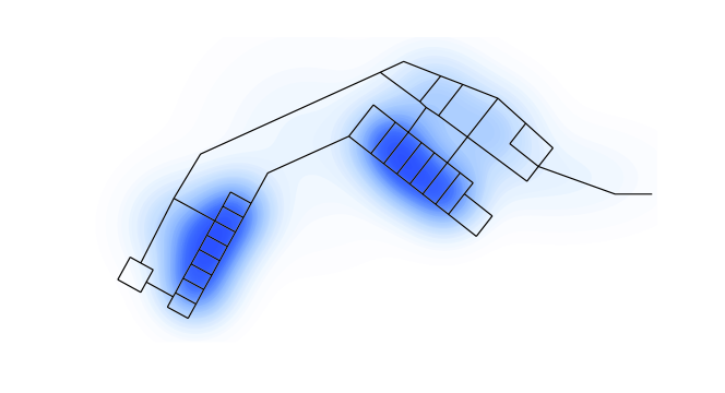
Figure 1: Network representing a wing of the Amsterdam Schiphol airport and contour plot of the density function $\phi$ used in simulations (darker colors denote preferential areas).

The $50$ sensors to be deployed have performance function $f(x)=\frac{1}{2}\left(1-\tanh\left(\frac{x-\frac{R}{2}}{\frac{R}{6}}\right)\right)$, where $R$ is a parameter considered as variable in the first step and as fixed in the second step of the optimization. Even if the previous function describes sensors with an infinite sensing radius, they will be represented as shaded circles of radius $\frac{7}{8}R$ to emphasize that the performance function assumes values lesser than $0.01$ for larger distances.

5.1 First step

The first step of the optimization is performed on a collapsed network with collapsing factor $r=0.3$ (see the small dots along the grey network in fig. 2-a,-c)). Sensors are grouped in $10$ clusters of $5$ elements each, and each cluster is represented as a single sensor. Clusters set initially $R=10$ and decrease linearly its value up to $1$ during the simulation (compare fig. 2-a) with fig. 2-c)). As apparent by the flows in fig. 2-b), clusters are allowed to move in $\mathbb{R}^{2}$.

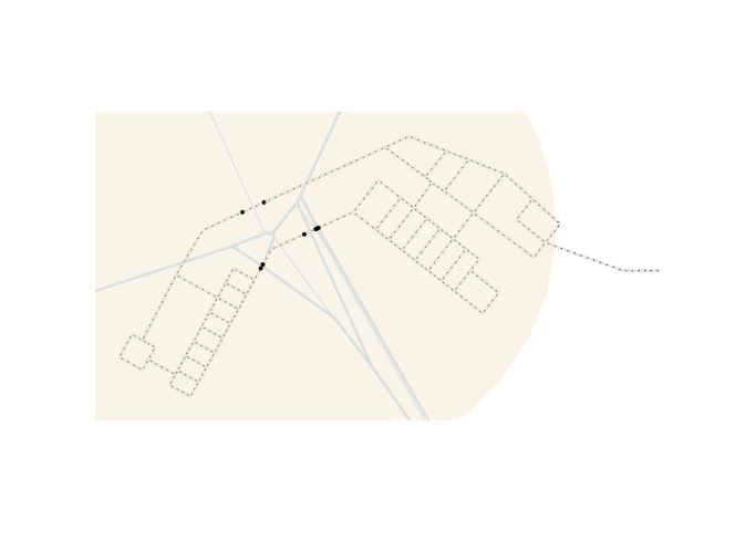
a)

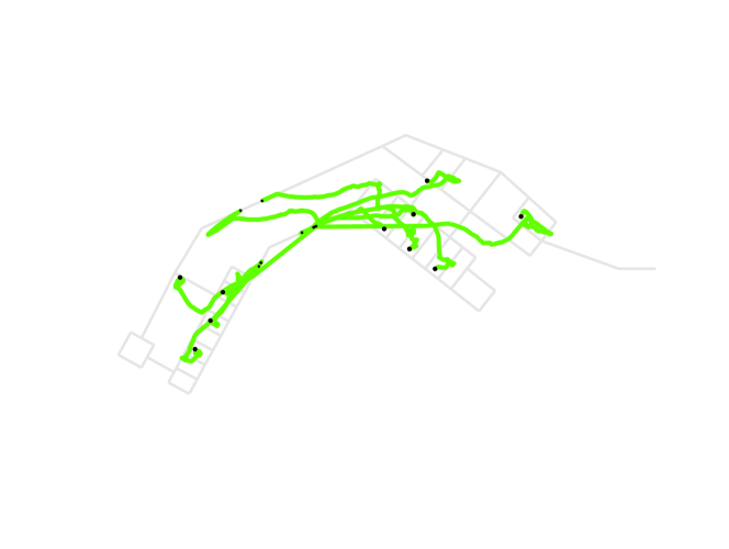
b)

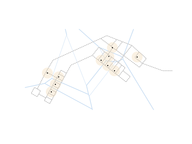
c)

Figure 2: First step of the optimization procedure for the deployment over a collapsed network of $50$ sensors grouped in $10$ clusters: a) initial positions of clusters (sensing radius $R=10$) and related Voronoi partition; b) gradient ascent flows (clusters allowed to move in $\mathbb{R}^{2}$); c) final positions, not necessarily belonging to the network, (sensing radius $R=1$) and related Voronoi partition.

It is important to recall that, both the variation of the sensing radius and the unconstrained motion of sensors are allowed in the first step as it is performed off-line. This step makes use of the algorithm described in section 3.1 and is thought to provide a good starting point for the second step. However, if sensors are initially located on the network as in fig. 2-a), they can execute the first step independently, using partial or rough information of the environment, without moving, and then plan a route on the network to reach the previously computed final positions. Since final positions can be not on the network (see fig. 2-c)), they must be projected on it to be reachable. Anyway, this projection has to be performed before the second step to provide a valid starting point.

5.2 Second step

The second step considers a full network with sensors having fixed radius $R=1$ and initially deployed in the positions shown in fig. 3-a). Such positions are obtained by spreading randomly $5$ sensors close to each cluster center and projecting them on the closest segments of the network. Sensors now can take real measures from the environment and perform the optimization on-line, while moving, according to the algorithm described in section 4. They are constrained to move on the network as shown in fig. 3-b). Final positions (see fig. 3-c)) show how sensors, originally clustered, diffused to better cover preferential areas (see fig 1).

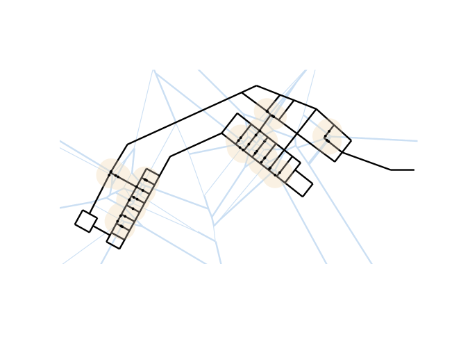
a)

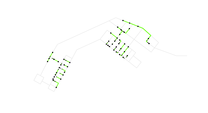
b)

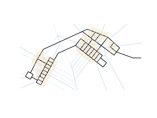
c)

Figure 3: Second step of the optimization procedure for the deployment of $50$ sensors with $R=1$ over a full network: a) initial positions obtained by spreading randomly $5$ sensors close to each cluster position found in the first step (see fig. 2-c)) and then projecting them on the network, related Voronoi partition; b) gradient ascent flows (sensors constrained to move on the network); c) final positions and related Voronoi partition.

6 Conclusions and Future Works

This paper focused on the problem of optimally deploying sensors in an environment modeled as a network. An optimization problem for the allocation of omnidirectional sensors with potentially limited sensing radius has been formulated. A novel two-step optimization procedure based on a discrete-time gradient ascent algorithm has been presented. In order the algorithm to not get stuck early in one of the many local minima, in the first (off-line) step, sensors are allowed to move in the plane. Moreover, a reduced model of the environment, called collapsed network, and sensors’ clustering, are used to speed up the first optimization. The positions found in the first step are then projected on the network and used in the second (on-line) finer optimization, where sensors are constrained to move only on the network.

The proposed procedure can be used to solve both static and dynamic deployment problems and the first step alone can provide solutions to location-allocation problems involving facilities located in the interior of the network.

A main future research direction will consider the integration of classical Operative Research methods with the present gradient algorithm. In particular the first optimization could be addressed by adapting methods and heuristics developed for the solution of the multisource Weber problem ([2]). The aim is to build an overall global optimization technique to solve location-allocation problems of large dimensions with many facilities. Moreover, future research, more related to deployment problems, will consider other sensor’s models such as those with limited sensing cone.

Appendix A

Theorem 19

Let $\varphi:\mathbb{R}^{2}\times\mathbb{R}_{+}\rightarrow\mathbb{R}$ be a smooth function w.r.t. its second argument and a non-increasing, piecewise differentiable map with a finite number of bounded discontinuities at $R_{1},\ldots,R_{N}\in\mathbb{R}_{+}$, $R_{1}<\ldots<R_{N}$, w.r.t. its first argument. Let $\nu:\mathbb{R}^{2}\times\mathbb{R}^{2}\rightarrow\overline{\mathbb{R}}_{+}$ be a continuously differentiable map w.r.t. both its arguments. Let $s=[a,b]\subset\mathbb{R}^{2}$ be a segment and assume that

i)

$\nu(\bar{x},a),\nu(\bar{x},b)\notin\left\{R_{1},\ldots,R_{N}\right\}$;

ii)

$\forall q\in[a,b]$, if $\nabla\nu(\bar{x},q)\cdot(b-a)=0\Rightarrow\nu(\bar{x},q)\notin\left\{R_{1},\ldots,R_{N}\right\}$,

then

$$\frac{d}{dx}\left.{\displaystyle\int\nolimits_{s}}\varphi\left(\nu\left(x,q\right),q\right)dq\right|_{x=\bar{x}}$$

$$={\displaystyle\int\nolimits_{[0,1]\backslash\left\{t_{1,1},\ldots,t_{1,k_{1}},\ldots,t_{N,1},\ldots,t_{N,k_{N}}\right\}}}\frac{\partial}{\partial\nu}\varphi(\nu(\bar{x},\gamma(t)),\gamma(t))\left.\frac{\partial\nu(x,\gamma(t))}{\partial x}\right|_{x=\bar{x}}\left\|b-a\right\|dt$$

$$+{\displaystyle\sum\limits_{i=1}^{N}}{\displaystyle\sum\limits_{j=1}^{k_{i}}}\left(\varphi(R_{i}^{+},\gamma(t_{i,j}))-\varphi(R_{i}^{-},\gamma(t_{i,j}))\right)\left.\frac{\partial\nu(x,\gamma(t))}{\partial x}\right|_{\begin{subarray}{c}x=\bar{x}\\ t=t_{i,j}\end{subarray}}\left\|b-a\right\|\text{,}$$

where $\gamma(t)=a+\left(b-a\right)t,$ $t\in[0,1]$ is a parameterization for $s$ and $t_{i,j}\in[0,1],~{}j\in\{1,\ldots,k_{i}\}$ are the zeros of $\nu(\bar{x},\gamma(t))-R_{i}=0$.

Proof. By using the Dirac’s delta formalism we have

$$\frac{d}{dx}\left.{\displaystyle\int\nolimits_{s}}\varphi\left(\nu\left(x,q\right),q\right)dq\right|_{x=\bar{x}}$$

$$=\left.{\displaystyle\int\nolimits_{s}}\frac{\partial}{\partial x}\varphi(\nu(x,q),q)dq\right|_{x=\bar{x}}$$

$$={\displaystyle\int\nolimits_{s}}\left.\frac{\partial}{\partial\nu}\varphi(\nu(x,q),q)\right|_{\nu\notin\left\{R_{1},\ldots,R_{N}\right\}}\left.\frac{\partial\nu(x,q)}{\partial x}\right|_{x=\bar{x}}dq$$

$$+{\displaystyle\int\nolimits_{s}}{\displaystyle\sum\limits_{i=1}^{N}}\left(\varphi(R_{i}^{+},q)-\varphi(R_{i}^{-},q)\right)\delta\left(\nu-R_{i}\right)\left.\frac{\partial\nu(x,q)}{\partial x}\right|_{\nu=R_{i}}dq\text{.}$$

With the chosen parameterization of $s$, the equation $\nu(\bar{x},\gamma(t))-R_{i}=0$ may have $k_{i}$ zeros $t_{i,j}\in[0,1],~{}j\in\{1,\ldots,k_{i}\}$. Thanks to i) and ii) the set of zeros $t_{i,j}$ does not change cardinality for $x$ near $\bar{x}$, thus, $t_{i,j}$ depends smoothly on $x$. Recalling that for every arc $\gamma:[l,u]\rightarrow\Gamma$ we have

$${\displaystyle\int\nolimits_{\Gamma}}f(x)dx={\displaystyle\int\nolimits_{l}^{u}}f(\gamma(t))\left\|\dot{\gamma}(t)\right\|dt\text{,}$$

and that for the special case of $s$ $\left\|\dot{\gamma}(t)\right\|=\left\|b-a\right\|$, the derivative becomes

$$\frac{d}{dx}\left.{\displaystyle\int\nolimits_{s}}\varphi\left(\nu\left(x,q\right),q\right)dq\right|_{x=\bar{x}}$$

$$={\displaystyle\int\nolimits_{[0,1]\backslash\left\{t_{1,1},\ldots,t_{1,k_{1}},\ldots,t_{N,1},\ldots,t_{N,k_{N}}\right\}}}\frac{\partial}{\partial\nu}\varphi(\nu(\bar{x},\gamma(t)),\gamma(t))\left.\frac{\partial\nu(x,\gamma(t))}{\partial x}\right|_{x=\bar{x}}\left\|b-a\right\|dt$$

$$+{\displaystyle\int\nolimits_{[0,1]}}{\displaystyle\sum\limits_{i=1}^{N}}\left(\varphi(R_{i}^{+},\gamma(t))-\varphi(R_{i}^{-},\gamma(t))\right)\delta\left(\nu-R_{i}\right)\left.\frac{\partial\nu(x,\gamma(t))}{\partial x}\right|_{\nu=R_{i}}\left\|b-a\right\|dt\text{,}$$

from which, using the property ${\displaystyle\int\nolimits_{l}^{u}}f(x)\delta\left(x-\bar{x}\right)dx=f(\bar{x})$ for $\bar{x}\in[l,u]$, we have the thesis.

References

- [1] V. S. Borkar. Stochastic approximation: A dynamical systems viewpoint. Cambridge University Press, 2008.
- [2] J. Brimberg, P. Hansen, N. Mladenović, and E. C. Taillard. Improvements and comparison of heuristics for solving the uncapacitated multisource Weber problem. Operations Research, 48(3):444–460, 2000.
- [3] C. H. Caicedo-Núñez and M. Žefran. Performing coverage on nonconvex domains. In 17th IEEE Int. Conf. on Control Applications, pages 1019–1024, Sept. 2008.
- [4] P. Cappanera. A survey on obnoxious facility location problems. Technical Report TR-99-11, Dept. of Informatics - Univ. of Pisa, April 1999.
- [5] J. Cortés and F. Bullo. Coordination and geometric optimization via distributed dynamical systems. SIAM J. Contr. Optim., 44(5):1543–1574, 2005.
- [6] J. Cortés, S. Martínez, and F. Bullo. Spatially-distributed coverage optimization and control with limited-range interactions. ESAIM Contr. Optim. & Calc. of Variations, 11:691–719, 2005.
- [7] J. Cortés, S. Martínez, T. Karataş, and F. Bullo. Coverage control for mobile sensing networks. IEEE Trans. Robot. and Automat., 20(2):243–255, 2004.
- [8] T. Drezner and Z. Drezner. Location of a facility in a planar network. In 38th SWDSI Annual Conf., San Diego, CA, USA, 13–17 March 2007.
- [9] Z. Drezner. Facility Location: A Survey of Applications and Methods. Series in Operations Research. Springer Velag, New York, 1995.
- [10] Z. Drezner and A. Suzuki. The big triangle small triangle method for the solution of nonconvex facility location problems. Operations Research, 52(1):128–135, 2004.
- [11] Q. Du, V. Faber, and M. Gunzburger. Centroidal Voronoi tessellations: Applications and algorithms. SIAM Rev., 41(4):637–676, 1999.
- [12] E. Erkut and S. Neuman. Analytical models for locating undesirable facilities. Eur. J. Oper. Res., 40(3):275–291, 1989.
- [13] A. Ganguli, S. Susca, S. Martínez, F. Bullo, and J. Cortés. On collective motion in sensor networks: Sample problems and distributed algorithms. In Proc. IEEE Int. Conf. on Decision and Control and Eur. Control Conference, pages 4239–4244, Seville, Spain, December 2005.
- [14] C. Gao, J. Cortés, and F. Bullo. Notes on averaging over acyclic digraphs and discrete coverage control. Automatica, 44(8):2120–2127, 2008.
- [15] Z. Guo, M. Zhou, and G. Jiang. Adaptive sensor placement and boundary estimation for monitoring mass objects. IEEE Trans. Syst. Man and Cyber. – Part B: Cybernetics, 38(1):222–232, Feb. 2008.
- [16] N. Heo and P. K. Varshney. Energy-efficient deployment of intelligent mobile sensor networks. IEEE Trans. Syst. Man and Cyber. – Part A, 35(1):78–92, Jan. 2005.
- [17] A. Howard, M. J. Matarić, and G. S. Sukhatme. Mobile sensor network deployment using potential fields: A distributed, scalable solution to the area coverage problem. In H. Asama, T. Arai, T. Fukuda, and T. Hasegawa, editors, Proc. 6th Int. Symp. on Distrib. Auton. Rob. Systems, pages 299–308. Springer, 2002.
- [18] A. Jadbabaie, J. Lin, and A. S. Morse. Coordination of groups of mobile autonomous agents using nearest neighbor rules. IEEE Trans. Automat. Contr., 48(6):988–1001, 2003.
- [19] A. Krause, C. Guestrin, A. Gupta, and J. Kleinberg. Near-optimal sensor placements: Maximizing information while minimizing communication cost. In Proc. of Inf. Processing in Sensor Networks, 2006.
- [20] A. Krause, J. Leskovec, C. Guestrin, J. VanBriesen, and C. Faloutsos. Efficient sensor placement optimization for securing large water distribution networks. J. of Water Resources Plan. and Manag., 134(6):516–526, 2008.
- [21] A. Krause, R. Rajagopal, A. Gupta, and C. Guestrin. Simultaneous placement and scheduling of sensors. In Proc. ACM/IEEE Int. Conf. on Inf. Processing in Sensor Networks, 2009.
- [22] H. J. Kushner and G. Yin. Stochastic approximation and recursive algorithms and applications. Springer, 2003.
- [23] S. P. Lloyd. Least squares quantization in PCM. IEEE Trans. Inf. Theory, 28(2):129–137, 1982.
- [24] Y. Mao and M. Wu. Coordinated sensor deployment for improving secure communications and sensing coverage. In 3rd ACM Wor. On Security of Ad Hoc and Sensor Networks, pages 117–128, Alexandria, VA, USA, Nov. 2005. ACM Press New York, NY, USA.
- [25] S. Martínez, J. Cortés, and F. Bullo. Motion coordination with distributed information. IEEE Contr. Syst. Mag., 27(4):75–88, 2007.
- [26] N. Mladenović, J. Brimberg, P. Hansen, and J. A. Moreno-Pérez. The -median problem: A survey of metaheuristic approaches. Eur. J. Oper. Res., 179(3):927–939, 2007.
- [27] A. Okabe and A. Suzuki. Locational optimization problems solved through Voronoi diagrams. Eur. J. Oper. Res., 98(3):445–456, 1997.
- [28] P. Sharma, S. Salapaka, and C. Beck. A scalable deterministic annealing algorithm for resource allocation problems. In Proc. American Control Conf., pages 3092–3097, Minneapolis, MN, USA, 14–16 June 2006.
- [29] A. Suzuki and Z. Drezner. The -center location problem in an area. Location Science, 4(1-2):69–82, 1996.
- [30] B. C. Tansel, R. L. Francis, and T. J. Lowe. Location on networks: A survey. Part I: The -center and -median problems. Manag. Science, 29(4):482–497, 1983.
- [31] B. C. Tansel, R. L. Francis, and T. J. Lowe. Location on networks: A survey. Part II: Exploiting tree network structure. Manag. Science, 29(4):498–511, 1983.
- [32] J. N. Tsitsiklis, D. P. Bertsekas, and M. Athans. Distributed asynchronous deterministic and stochastic gradient optimization algorithms. IEEE Trans. Automat. Contr., 31(9):803–812, Sep. 1986.
- [33] Y. Zou and K. Chakrabarty. Sensor deployment and target localization in distributed sensor networks. ACM Trans. Embedded Computing Sys., 3(1):61–91, 2004.