Non-thermal radio emission from O-type stars

Abstract

Context. Several early-type colliding-wind binaries are known to emit synchrotron radiation due to relativistic electrons, which are most probably accelerated by the Fermi mechanism. By studying such systems we can learn more about this mechanism, which is also relevant in other astrophysical contexts. Colliding-wind binaries are furthermore important for binary frequency determination in clusters and for understanding clumping and porosity in stellar winds.

Aims. We study the non-thermal radio emission of the binary Cyg OB2 No. 8A, to see if it is variable and if that variability is locked to the orbital phase. We investigate if the synchrotron emission generated in the colliding-wind region of this binary can explain the observations and we verify that our proposed model is compatible with the X-ray data.

Methods. We use both new and archive radio data from the Very Large Array (VLA) to construct a light curve as a function of orbital phase. We also present new X-ray data that allow us to improve the X-ray light curve. We develop a numerical model for the colliding-wind region and the synchrotron emission it generates. The model also includes free-free absorption and emission due to the stellar winds of both stars. In this way we construct artificial radio light curves and compare them with the observed one.

Results. The observed radio fluxes show phase-locked variability. Our model can explain this variability because the synchrotron emitting region is not completely hidden by the free-free absorption. In order to obtain a better agreement for the phases of minimum and maximum flux we need to use stellar wind parameters for the binary components which are somewhat different from typical values for single stars. We verify that the change in stellar parameters does not influence the interpretation of the X-ray light curve. Our model has trouble explaining the observed radio spectral index. This could indicate the presence of clumping or porosity in the stellar wind, which – through its influence on both the Razin effect and the free-free absorption – can considerably influence the spectral index. Non-thermal radio emitters could therefore open a valuable pathway to investigate the difficult issue of clumping in stellar winds.

1 Introduction

All hot stars emit radio radiation due to thermal free-free emission by the ionized material in their stellar wind. A number of those stars also show non-thermal radio emission that dominates the thermal component. This non-thermal emission is believed to be due to electrons that are Fermi-accelerated around shocks (Bell 1978). As these relativistic electrons spiral around in the magnetic field, they emit synchrotron radiation, which we detect as non-thermal radio emission (Bieging et al. 1989).

Two hypotheses have been proposed for the origin of the shocks responsible for the non-thermal emission. These shocks could be due to the collision of the two winds in a binary system (Eichler & Usov 1993; Dougherty et al. 2003; Pittard et al. 2006; Reimer et al. 2006), or they could be formed by the radiative instability mechanism in the wind of a single star (Owocki & Rybicki 1984; Chen & White 1994). The binary hypothesis is supported by the non-thermal Wolf-Rayet stars (Dougherty & Williams 2000) and by a number of known O+O binaries showing non-thermal radio emission (e.g. Cyg OB2 No. 5; Contreras et al. 1997). The single-star hypothesis, on the other hand, is supported by a number of seemingly single O stars showing non-thermal radio emission.

In recent years, however, doubt has been cast on the single-star hypothesis. In previous papers of this series, we have shown that the radio emission for some of these stars shows periodic variability, suggesting binarity (HD 168 112 and Cyg OB2 No. 9; Blomme et al. 2005; Van Loo et al. 2008). Optical spectroscopy has shown that a number of these “single” stars are actually binaries (e.g. Cyg OB2 No.~8A and No. 9; De Becker et al. 2004; Nazé et al. 2008). Furthermore, theoretical work by Van Loo et al. (2006) showed that non-thermal radio radiation from a single star would be unlikely, as the synchrotron emission would be largely absorbed by the stellar wind material.

The study of colliding-wind systems is important for a number of reasons. First, because we can learn more about the Fermi acceleration mechanism, which is relevant to a wide range of astrophysical objects such as interplanetary shocks and supernova remnants (e.g. Jones & Ellison 1991). The physical conditions in a colliding-wind binary are quite different from those in other objects. The different range of density, magnetic field and radiation environment in these binaries provides substantial new information on the acceleration mechanism. Models, constrained by radio data, also provide predictions for the expected gamma-ray flux from these systems. These numbers are important for observations of colliding-wind binaries by current and future high-energy instruments, both ground-based and space-based ones (e.g. INTEGRAL, IXO, HESS, VERITAS).

Furthermore, the non-thermal radio emitters are useful for improving the determination of the binary frequency in clusters. The colliding-wind binaries allow us to find the longer-period systems, which are easy to detect at radio wavelengths but much harder to find with standard spectroscopic observing techniques.

Finally, colliding-wind systems are also highly relevant for mass-loss rate determinations in single stars. This has become a major problem in massive star research in recent years due to the fact that winds are clumped and porous. Taking into account clumping decreases the mass loss rates by a factor $3-10$ compared to what was previously thought (e.g. Puls et al. 2008). By determining how much of the synchrotron radiation emitted at the colliding-wind region is absorbed by the stellar wind material, we can estimate the amount of porosity in the wind.

In this paper we study the non-thermal radio emission of the colliding-wind binary Cyg OB2 No. 8A (RA = 20h33m15$\aas@@fstack{s}$0789, Dec = +41°18’50$\aas@@fstack{\prime\prime}$494, J2000). We also present additional X-ray observations that improve the X-ray light curve presented by De Becker et al. (2006). Cyg OB2 No. 8A is undoubtedly the O + O non-thermal radio emitter with the best constrained stellar, wind and orbital parameters so far (De Becker 2007). It has been known as a non-thermal radio emitter since the first major survey of O star radio emission by Bieging et al. (1989). It was recognized as such by its clearly negative spectral index. This system was only recently discovered to be a binary by De Becker et al. (2004). It consists of an O6If primary and an O5.5III(f) secondary. It has a period of 21.908 $\pm$ 0.040 d and an eccentricity of 0.24 $\pm$ 0.04. All binary parameters were determined by De Becker et al. (2006) and are listed in Table 1.

Table 1: Parameters of Cyg OB2 No. 8A used in this work.

Parameter	Primary	Secondary
$T_{\rm eff}$ (K)	36800	39200
$R_{*}$ ($R_{\sun}$)	20.0	14.8
$M_{*}$ ($M_{\sun}$)	44.1	37.4
log $L_{\rm bol}/L_{\sun}$	5.82	5.67
$\dot{M}$ ($M_{\sun}{\rm yr}^{-1}$)	$4.8\times 10^{-6}$	$3.0\times 10^{-6}$
$\varv_{\infty}$ (km s-1)	1873	2107
semi-major axis $a$ ($R_{\sun}$)	65.7	76.0
period $P$ (days)	$21.908\pm 0.040$
eccentricity $e$	$0.24\pm 0.04$
inclination $i$	$32\degr\pm 5\degr$
distance $D$ (kpc)	1.8

Table 2: Two new X-ray observations of Cyg OB2 No. 8A.

Phase	Rev.	Obs. ID	Date	JD	Exp. Time				Count Rates
					(s)				(counts s-1)
					MOS1	MOS2	pn		MOS1	MOS2	pn
0.155	1353	0505110301	2007 Apr 29	4220.417	26879	27149	20581		0.655$\pm$0.006	0.640$\pm$0.005	1.892$\pm$0.012
0.326	1355	0505110401	2007 May 03	4224.167	27065	29155	22116		0.734$\pm$0.006	0.730$\pm$0.006	2.114$\pm$0.011

Table 3: Parameters for the two new EPIC spectra of Cyg OB2 No. 8A.

Instr.	Log $N_{\mathrm{w}}$	$kT_{1}$	Norm1	$kT_{2}$	Norm2	$kT_{3}$	Norm3	$\chi^{2}_{\nu}$ (d.o.f.)	Obs.Flux
		(keV)	(10-2)	(keV)	(10-3)	(keV)	(10-3)		(erg cm-2 s-1)
Observation 5
MOS1	21.79${}_{21.68}^{21.87}$	0.26${}_{0.23}^{0.30}$	3.43${}_{1.39}^{6.76}$	0.78${}_{0.72}^{0.87}$	7.81${}_{6.43}^{9.47}$	1.73${}_{1.60}^{1.90}$	6.33${}_{5.31}^{7.24}$	1.28 (230)	5.28 $\times$ 10-12
pn	21.86${}_{21.80}^{21.91}$	0.25${}_{0.23}^{0.29}$	6.06${}_{3.43}^{10.10}$	0.84${}_{0.79}^{0.89}$	10.96${}_{9.48}^{12.44}$	1.86${}_{1.71}^{2.06}$	4.96${}_{3.91}^{5.94}$	0.93 (436)	5.69 $\times$ 10-12
EPIC	21.81${}_{21.77}^{21.86}$	0.27${}_{0.25}^{0.29}$	3.72${}_{2.48}^{5.78}$	0.81${}_{0.77}^{0.86}$	8.85${}_{7.93}^{9.90}$	1.77${}_{1.68}^{1.88}$	5.80${}_{5.09}^{6.44}$	1.36 (691)	5.49 $\times$ 10-12
Observation 6
MOS1	21.80${}_{21.72}^{21.84}$	0.22${}_{0.20}^{0.24}$	8.14${}_{4.66}^{12.20}$	0.89${}_{0.82}^{0.99}$	7.02${}_{5.79}^{8.64}$	1.60${}_{1.51}^{1.75}$	7.96${}_{6.12}^{9.20}$	1.78 (329)	6.00 $\times$ 10-12
pn	21.73${}_{21.68}^{21.77}$	0.26${}_{0.24}^{0.28}$	3.83${}_{2.70}^{5.50}$	0.79${}_{0.76}^{0.82}$	9.70${}_{8.86}^{1.79}$	10.56${}_{1.67}^{1.79}$	7.75${}_{7.24}^{8.23}$	1.11 (843)	6.72 $\times$ 10-12
EPIC	21.70${}_{21.67}^{21.72}$	0.26${}_{0.25}^{0.28}$	3.17${}_{2.53}^{3.84}$	0.81${}_{0.78}^{0.84}$	7.60${}_{7.06}^{8.14}$	1.68${}_{1.63}^{1.72}$	8.07${}_{7.66}^{8.45}$	1.96 (1274)	6.39 $\times$ 10-12

De Becker et al. (2006) studied the X-ray emission of this binary. They found an essentially thermal spectrum, but with an overluminosity of a factor $19-28$ compared to the canonical $L_{X}/L_{\rm bol}$ ratio for non-interacting O-type stars. This overluminosity is due to additional X-ray emission by material heated in the colliding-wind region. The X-ray light curve shows variability of $\sim$ 20 %. Although the curve is not well sampled, it suggests that the variability is phase-locked.

In Sect. 2 we present the radio continuum observations of Cyg OB2 No. 8A and in Sect. 3 the new X-ray data. The model for the synchrotron radio emission in a colliding-wind binary is described in Sect. 4. In Sect. 5 we apply this model both for a standard set of star and wind parameters and an alternative set chosen to obtain better agreement with the data. Conclusions are given in Sect. 6.

2 Radio data

We obtained a number of 6 cm continuum observations of Cyg OB2 No. 8A with the NRAO Very Large Array (VLA) during 2005 February 04 to March 12, covering about 1.6 orbital periods. We also retrieved a considerable number of observations from the VLA archive (also covering other wavelengths), which we used in the present analysis. To avoid introducing systematic effects, we re-reduced the archive data in the same way as our own data (see Appendix B). The resulting fluxes and their error bars are listed in Table B.

In Fig. 1, we plot a subset of these fluxes. We limit the figure to the 3.6 and 6 cm data as the other wavelengths have only a few observations or detections. We do not plot fluxes which were measured on images where Cyg OB2 No. 8A was offset from the centre. Though these observations follow the same general trend as the “on-centre” observations, they usually have large error bars and would therefore considerably confuse the figure.

Figure 1 shows clear variability in the fluxes which is phase-locked with the orbital period. This is especially obvious at the 6 cm wavelength which has the most data. Maximum flux is at phase $\sim$ 0.1 (where the primary is in front). The phase of minimum flux is less well determined due to a gap in the phase coverage, but is at $\sim$ 0.6 (close to where the secondary is in front). To check that the variability is not an instrumental effect, we also measured two other targets on the images: Cyg~OB2 No.~63 and No. 9. Although these are also variable (No. 9, see Van Loo et al. 2008), their variability is not correlated with the No. 8A variability. We can therefore exclude instrumental effects.

Only a few simultaneous observations at more than one wavelength are available to study the spectral index. We find that before phase 0.5, the 3.6 and 6 cm fluxes are roughly equal, corresponding to a spectral index of about 0.0 (within the error bars). After phase 0.5, the fluxes behave differently: the 3.6 cm flux reaches higher values much more quickly than the 6 cm one, which translates into a spectral index of $\sim$ $+0.7$. Interestingly, this is close to the orbital phase where the only significantly negative spectral index ($\sim$ $-0.7$) is found, occurring between the 6 and 20 cm observations of programme AC116 (1984-12-21, phase = 0.51).

We next try to determine the period from the 6 cm data used in Fig. 1. To do so, we use the string-length method of Dworetsky (1983). The best period we find is 23.75 d, which is quite different from the 21.908-d value derived from optical spectroscopy (De Becker et al. 2004). However, the minimum in the string-length is not very significant. Furthermore, if we replot the De Becker et al. spectroscopic velocities on the 23.75-d period, we find that the points are scattered all over the diagram, indicating that the proposed radio period is clearly wrong. We therefore use the 21.908-d period in the further analysis.

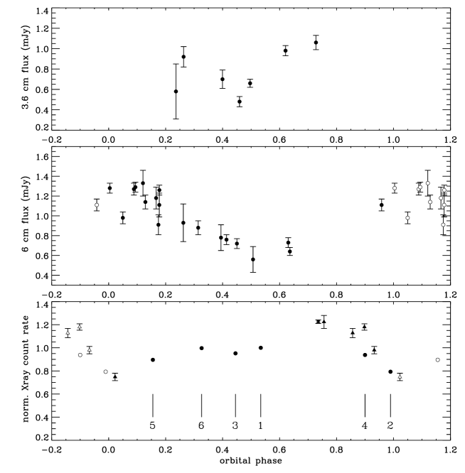
Figure 1: Radio and X-ray observations of Cyg OB2 No. 8A. The upper and middle panel show the 3.6 cm and 6 cm radio fluxes. We plot only those fluxes that were measured on-centre. All fluxes are plotted as a function of orbital phase in the 21.908-d period, with phase 0.0 corresponding to periastron. The lower panel shows the X-ray fluxes, with count rates that have been normalized on XMM-Newton observation no. 1 (see text). Triangles indicate ROSAT-PSPC observations, the cross the ASCA-SIS1 observation, and circles the XMM-Newton-EPIC data (these are also labelled by their observation number). Error bars are shown, except for the XMM-Newton data, as these are smaller than the symbol used. To better show the behaviour of the X-ray and radio light curves, we extend the phase range by 0.2 on either side; open symbols indicate duplications in that extended range.

3 X-ray data

Cyg OB2 No. 8A has been observed in X-rays two times with the XMM-Newton satellite since the publication of the De Becker et al. (2006) paper (Obs. ID 050511, PI: G. Rauw). These observations were scheduled in order to fill the gap in phase coverage of previous X-ray observations, and occurred during revolutions 1353 and 1355 (respectively at phases 0.155 and 0.326, see Table 2 for details). We adopted the same procedure as in De Becker et al. for the data processing using the Science Analysis Software (v.6.0.0), and we refer to this study for details. We note that we rejected short time intervals of high background due to soft proton flares. We fitted the new EPIC spectra with the same three-temperature model as used by De Becker et al. (2006) for previous XMM-Newton observations. The best fit parameters are given in Table 3; they are consistent with those derived for the four previous observations, even though some variability is detected for some of them.

In Fig. 2, we have plotted the parameters obtained from the best fit of EPIC data (MOS1 and pn) of the six XMM-Newton observations (see Table 4 in De Becker et al. (2006), and Table 3 in this paper) versus the orbital phase. The local absorption column density undergoes significant variability as a function of the orbital phase, with a maximum occurring close to periastron passage (phase 0.0). At that time the wind interaction region is behind the primary wind, which is likely to be responsible for a substantial absorption of X-rays. The plasma temperatures show only weak, or even no phase-locked variability. Only slight variations are suggested in the case of the hard emission component that might be related to the small changes in the pre-shock velocities as the separation between the stars changes along the eccentric orbit. The lower and higher temperature are indeed found, respectively, close to periastron and apastron for the hard component, but this trend should be considered with caution in view of the scatter and of the error bars of the measurements. Finally, the normalization parameters (which are related to the emission measure) undergo significant phase-locked variations, mostly if one considers the soft emission component that dominates the X-ray spectrum. The maximum coincides remarkably with orbital phases close to periastron, in agreement with the idea that the maximum X-ray emission occurs when the emission measure is expected to be maximum.

Figure 2: Variation of the best fit parameters as a function of orbital phase ($\phi$), for all six EPIC X-ray spectra. Upper panel: local absorption components expressed in 10²² cm^-2. Middle panel: plasma temperature expressed in keV. Lower panel: normalization parameters expressed in units of 10^-3 cm^-5. In the middle and lower panels, the solid, dotted and dashed lines stand, respectively, for the soft, the medium and the hard emission components of the composite model.

We proceeded following the same approach as in De Becker et al. (2006) to build a light curve including ROSAT-PSPC, ASCA-SIS and XMM-Newton-EPIC data (see their Fig. 6). In order to consistently compare the count rates obtained with different instruments, we used the first XMM-Newton observation as a reference (obs. 1 in De Becker et al., obtained at orbital phase 0.534). We used the 3-temperature model with the parameters obtained for the simultaneous fit of EPIC-MOS1 and EPIC-pn data of that observation, and we convolved it with the respective response matrices of ROSAT-PSPC and ASCA-SIS1 to obtain faked spectra. We then normalized the count rates of the ROSAT and ASCA observations using the count rate of the reference fake spectrum in each case, thereby deriving the normalized count rates plotted in Fig. 1. It is interesting to note that the X-ray emission level at orbital phases 0.155 and 0.326 (respectively no. 5 and no. 6 in the XMM-Newton series) is not lower than at other orbital phases. This suggests that the X-ray minimum occurs very close to periastron.

An important result of Fig. 1 is that the X-ray and radio light curves are nearly anti-correlated. X-ray flux minimum occurs close to periastron, when the radio 6 cm flux is approaching maximum. Minimum radio flux is near phase 0.6, where the X-ray flux has increased well above its minimum value (though it has not yet reached maximum). The anti-correlation will present a challenge to modelling this binary system. Although we do not model the X-ray observations in the present paper, we discuss this point further in Sect. 5.3.

4 Modelling the radio fluxes

Blomme (2005) made a very simplified model for the radio emission of the Cyg OB2 No. 8A binary system. This model consists of a point-source synchrotron emitting region orbiting a single star inside a stellar wind that includes free-free absorption. The model shows that all synchrotron emission would be absorbed by the stellar wind material and that therefore the radio fluxes should not show phase-locked variability. Only by introducing a considerable amount of porosity in the stellar wind material does the non-thermal radio emission become detectable (due to the reduction in free-free absorption).

Here we present a more sophisticated model of Cyg OB2 No. 8A that takes into account the geometric extent of the colliding-wind region, as well as the acceleration, advection and cooling of the relativistic electrons. In this section we provide an outline of the model; for details we refer to Appendix A.

The present model does not solve the hydrodynamical equations, but instead uses the Antokhin et al. (2004) equations to define the position of the contact discontinuity that separates the two stellar winds. Estimates by De Becker et al. (2006, their Table 11) show the ratio of cooling time to the flow time to be around 1. At least during part of the orbit, the shocks can therefore be expected to be radiative, resulting in considerable variability and structure. Such complications are neglected in our model.

Next we assume that the contact discontinuity and the shocks on either side of it are sufficiently close to one another that we can consider them to be in the same geometric place. We then generate new relativistic electrons at the shocks and follow their time evolution as they advect and cool, till they no longer emit significant synchrotron radiation at the wavelength we are considering.

At the shock, the new electrons have a momentum distribution that is a power law modified for the effect of inverse Compton cooling. The number of relativistic electrons is determined by $\zeta$, the fraction of the energy that is transferred from the shock to the relativistic electrons. We assume the typical value of $\zeta=0.05$ (Blandford & Eichler 1987; Eichler & Usov 1993). The time evolution of the electrons is followed as they advect outward along the contact discontinuity and as they cool down due to inverse Compton and adiabatic cooling.

At each point along the tracks followed by the electrons, the synchrotron emissivity $j_{\nu}(r)$ can then be calculated. We include the Razin effect, which takes into account the effect of the non-relativistic plasma on the synchrotron emission. This emissivity is then mapped from the two-dimensional orbital plane on which it was defined on to a three-dimensional volume by rotating it along the line connecting both components of the binary. Note that this assumption of cylindrical symmetry neglects any effects due to orbital motion. We refer to Lemaster et al. (2007), Parkin & Pittard (2008) and Pittard (2009) for studies of the orbital motion effects in colliding-wind systems in general. Specifically for the relatively short-period system Cyg OB2 No. 8A, not taking into account orbital motion is a major assumption, and we discuss its effect in Sect. 5.2.

The model also includes the thermal free-free opacity and emissivity due to the ionized wind material. The winds are assumed to be smooth, i.e. no clumping or porosity effects are included. The model does not include the contribution due to the increased density and temperature in the colliding-wind region (contrary to Pittard 2010) as these hydrodynamical quantities are not calculated in our model. Radiative transfer is then solved in the three-dimensional simulation volume using Adam’s finite volume method (Adam 1990).

5 Results

The intention of our modelling is to see if we can reproduce qualitatively the main features of the observed Cyg OB2 No. 8A radio light curve (see Sect. 2). These are: (1) the fact that there is variability, (2) maximum flux is around phase 0.1, minimum flux around phase 0.6, and (3) the 3.6 cm and 6.0 cm fluxes are approximately equal, most of the time (i.e. spectral index $\approx 0$). We do not make a formal best fit as we consider the absolute values of the fluxes to be less important, since these are sensitive to many of the assumptions in the model (e.g. magnetic field, $\zeta$).

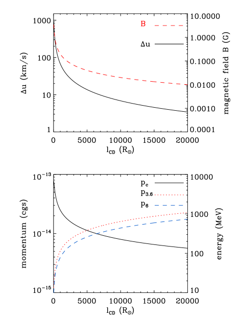
Figure 3: Upper panel: The jump in velocity at the shock ($\Delta u$, solid line) as a function of distance along the contact discontinuity ($l_{\rm CD}$). Also plotted is the magnetic field ($B$, dotted line). Lower panel: The maximum momentum ($p_{\rm c}$) due to inverse Compton cooling of the electrons accelerated at the shock, as a function of distance (solid line). Also plotted are the characteristic momenta for emission at 3.6 cm (dotted line) and 6 cm (dashed line). All data presented here are for the wind of the primary component of the binary, at periastron.

5.1 Standard model

5.1.1 Model details

The standard model uses the parameters listed in Table 1. We recall that De Becker et al. (2006) derived these from stellar parameters typical for single stars with the same spectral type as the binary components of Cyg OB2 No. 8A. We assume a surface magnetic field for each star of $B=100$ G, which is compatible with the fact that the magnetic field of most O-type stars is below detectable levels (e.g. Schnerr et al. 2008). The magnetic field at the shocks is directly related to this surface magnetic field (see Eq 9 and Fig. 3, upper panel); this neglects any amplification of the field (such as described by, e.g. Bell 2004) or any reduction of it by magnetic reconnection. As the true rotational velocity is not known, we make the assumption that $\varv_{\rm rot}/\varv_{\infty}=0.1$.

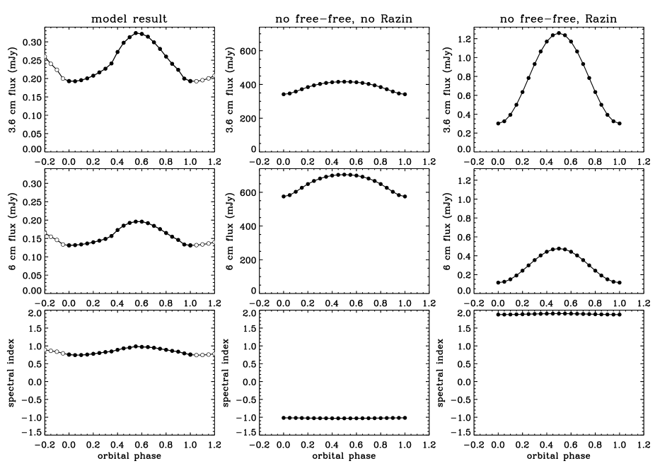
Figure 4: Results for the standard model. The left column shows the 3.6 cm (upper panel) and 6 cm fluxes (middle panel), as well as the spectral index between those wavelengths (lower panel). The middle column shows the same model, but we switched off the Razin effect and the free-free absorption and emission. The right column shows the intrinsic synchrotron emission, i.e. the Razin effect is included, but not the free-free absorption and emission. As for Fig. 1, open symbols indicate duplications in the extended phase range. Note the very different flux scales for the various panels.

A comparison between the $m\sin^{3}i$ values derived from the binary orbit and typical masses of single stars corresponding to the observed spectral types indicates an inclination angle of 32° (De Becker et al. 2006). For the free-free emission and absorption we take the material to be once ionized and assign it a temperature of 28 500 K ($\approx 0.75$ of the effective temperature of the stars). The three-dimensional simulation volume is a cube centred on the primary that is $40\,000\,R_{\sun}$ on each side and that consists of $256^{3}$ cells. Some care must be taken to use the appropriate resolution for a given size of the simulation box; we checked that the results presented here are robust to changes in size and resolution. The size of the box is large enough to contain most, but not all, of the emission. Doubling the size and using $512^{3}$ cells shows that the flux loss is less than 10 %, and that the shape of the radio light curve remains the same. With the resolution we use for the three-dimensional simulation volume, the apex of the contact discontinuity is not well resolved. This is of no consequence for our purpose, however, as the synchrotron emission coming from around the apex is completely absorbed by the free-free absorption (see also Sect. A.7).

5.1.2 Fluxes and spectral index

Figure 4 (left column) shows the resulting 3.6 cm and 6 cm fluxes as well as the spectral index between these two wavelengths. The first thing to note is that the model fluxes do show phase-locked variability, contrary to the simple point-source model (Blomme 2005). This is due to the synchrotron emission extending much further out than the point-source approximation suggests. In Fig. 5 (left column) we plot the contribution to the flux as a function of distance to the primary. To determine each flux value on that figure we artificially set the synchrotron emission to zero beyond a certain distance and re-run the radiative transfer model. The figure makes clear that the main flux contribution comes from distances of $1000-3000\,R_{\sun}$. This corresponds to approximately $10-30$ times the separation between the two stars. The flux contribution that can be seen at small distances is due to free-free emission of the entire wind, which was not cut off in this procedure. On the figure we also indicate the distances from the star where optical depth 1 for the primary component is reached. We calculate these using the Wright & Barlow (1975) formalism and find them to be $1130\,R_{\sun}$ at 3.6 cm and $1620\,R_{\sun}$ at 6 cm. As expected, the flux we receive is formed largely outside this radius.

Spatially resolved radio observations of colliding-wind regions typically do not show such an extended non-thermal region (e.g. WR 140; Dougherty et al. 2005). The present results are not in contradiction with this. The resolved observations show the surface brightness (flux per area) while the unresolved radio data presented here show the flux (i.e. integrated over a large area). At large distances from the centre of the binary system, the surface brightness decreases substantially, hence the relatively small extent of the colliding-wind region in resolved observations – which is nicely illustrated by the simulated data for WR 140 presented by Pittard & Dougherty (2006, their Fig. 17). But, as the synchrotron emission is cylindrically symmetric around the axis connecting the two stars, the low surface brightness at larger distances gets weighted with a much larger surface area and therefore contributes substantially to the flux.

While the phase-locked variability of the flux is a positive result for the model, unfortunately we find that the phases of minimum and maximum flux do not agree with the observations. The model results are nearly in anti-phase to the observations: theoretical maximum occurs at phase 0.55 (instead of the observed 0.1) and theoretical minimum at phase $0.0-0.05$ (instead of 0.6). Furthermore, the spectral index is not correctly predicted. The theoretical values of +0.75 to +1.0 do not agree with the observed values which are mostly close to 0.0 (Sect. 2).

5.1.3 Without Razin effect, without free-free absorption

To understand why the phases and spectral index are incorrectly modelled, we start by simplifying the model. When we leave out the free-free absorption and emission as well as the Razin effect, we find the light curve shown in the middle column on Fig. 4. The flux values are high ($\sim$ 700 mJy at 6 cm, $\sim$ 400 mJy at 3.6 cm). The spectral index is approximately $-1.0$, clearly indicating the non-thermal nature of the spectrum.

Figure 5: Cumulative contribution to the flux from synchrotron emission at various distances, for orbital phases 0.0 and 0.5. The left column shows the 3.6 cm (upper panel) and 6 cm fluxes (middle panel), as well as the spectral index between those wavelengths (lower panel). The dotted lines show where optical depth 1 is reached due to free-free absorption (for the wind of the primary component). The middle column shows the same model, but we switched off the Razin effect and the free-free absorption and emission. The right column shows the intrinsic synchrotron emission, which includes the Razin effect, but not the free-free absorption and emission. Note the very different flux scales for the various panels.

Fig. 5 (middle column) shows that in the model without Razin and without free-free absorption, the strongest contribution comes from relatively close to the apex (up to $\sim$ $300$ $R_{\sun}$, i.e. about $3$ times the binary separation). This is to be expected as the collision is strongest close to the apex, so more energy is available for the acceleration of the particles. On the other hand, inverse Compton cooling should be strongest there as well, leading to a reduction of the emission.

The resulting balance between acceleration and inverse Compton cooling can be seen in Fig. 3 (lower panel), where we plot the maximum momentum ($p_{\rm c}$) that can be reached due to inverse Compton cooling at the shock where the electrons are accelerated. We plot this value as a function of distance along the contact discontinuity ($l_{\rm CD}$). For comparison we also plot the “characteristic” momentum for 3.6 and 6 cm emission ($p_{6}$ and $p_{3.6}$), i.e. the momentum at which the synchrotron emission is largest for a given wavelength. Its value can be derived from the fact that maximum emission occurs at frequency $\nu=0.29\nu_{\rm s}$ (see, e.g. Van Loo 2005, Eq. 2.52), where $\nu_{\rm s}$ is given by Eq. 20. Close to the apex, $p_{\rm c}$ is considerably larger than $p_{6}$ (and $p_{3.6}$). Because of the (approximate) power-law distribution of the momentum, there are a large number of electrons available having their maximum emission at that wavelength. Moving towards the outer regions, $p_{\rm c}$ becomes closer to, or even lower than, $p_{6}$ (and $p_{3.6}$), thereby explaining the decrease of the emission.

Fig. 4 (middle column) shows that the maximum flux occurs at apastron (phase 0.5), the minimum at periastron (phase 0.0). At apastron, the stars are further apart and their winds have reached the highest speed before they collide. However, this effect cannot explain why maximum occurs at apastron. The energy available for the relativistic electrons is proportional to the shock energy $1/2\;\rho\varv^{2}$, which scales as $\varv/r^{2}$. The higher value for the velocity $\varv$ at apastron cannot compensate for the lower $1/r^{2}$ value. The main reason for maximum to occur at apastron is the (approximate) scale-invariance of the colliding-wind region. As the distance between the two stars becomes larger, the size of the synchrotron emitting region grows accordingly. Although the synchrotron emissivity is lower at apastron than at periastron, the integration over the larger size of the colliding-wind region results in a higher apastron flux.

5.1.4 With Razin effect, without free-free absorption

Next, we switch back on the Razin effect but we still leave out the free-free mechanism (Fig. 4 and 5, right column). This results in a substantial reduction of the flux levels (e.g. the 6 cm maximum flux goes down from $\sim$ 700 mJy to $\sim$ 0.4 mJy). The large influence of the Razin effect on the flux can be understood by making a few simple estimates. The crucial quantity is the factor $f$ defined in Eq. 18:

$$f(\nu,p)=\left[1+\frac{\nu_{0}^{2}}{\nu^{2}}\left(\frac{p}{m_{\rm e}c}\right)^{2}\right]^{-1/2},$$ (1)

where $\nu$ is the radio frequency, $m_{\rm e}$ the mass of the electron, $c$ the speed of light, $p$ the momentum of the electron and $\nu_{0}=\sqrt{n_{\rm e}e^{2}/(\pi m_{\rm e})}$. In the $\nu_{0}$ definition, $e$ is the charge of the electron and $n_{\rm e}$ is the number density of the thermal electrons (i.e. those of the non-relativistic plasma). The $f$-factor takes on values between 0 and 1 with $f=1$ indicating no effect, and $f\ll 1$ indicating a strong Razin effect. Taking the frequency at which the electron has its maximum emission, this translates into $\nu\ll\nu_{\rm R}$, where

$$\nu_{\rm R}=20\frac{n_{\rm e}}{B}$$ (2)

(see also Van Loo 2005, Eq. 2.53). We use Eq. 9 for the magnetic field $B$ and Eq. 22 to relate $n_{\rm e}$ to the mass density $\rho$. Determining $\rho$ from the mass-loss rate and approximating the velocity $\varv$ by the terminal velocity $\varv_{\infty}$ results in a $r^{-1}$ scaling of $\nu_{\rm R}$. Putting in the values for the primary (Table 1) and using for $\nu_{\rm R}$ the frequency corresponding to 6 cm, we find a critical radius of $\sim$ $1100$ $R_{\sun}$. The Razin effect is important below that radius, which is indeed where we see the largest effect in the model calculations (Fig. 5, comparing middle and right column).

In this model without free-free absorption, we note that the Razin effect does not change the position of maximum flux, which remains at phase 0.5. It does have an important effect on the spectral index, which becomes clearly positive ($\ga+1.9$). The large change in the spectral index can be explained by the frequency dependence of the Razin effect. The frequency dependence of $f$ (Eq. 1) is such that $f_{\rm 6cm}<f_{\rm 3.6cm}$, so the 6 cm flux is more affected than the 3.6 cm one. This leads to a strong change in the spectral index. Note that this change is highly sensitive to $n_{\rm e}$. To quantify this sensitivity, we calculate an artificial model without free-free absorption where we reduce the $n_{\rm e}$ value in the $\nu_{0}$ equation by a factor 30. This leads to a spectral index that is below 0.2 during that part of the orbit which is near flux maximum. We recall that the values used for $n_{\rm e}$ in our model (Eq. 22) are not based on hydrodynamics. The true values could therefore be very different, which will certainly influence the absolute fluxes as well as the spectral index.

The variability seen in Fig. 4 (right column) is phase-locked, with minimum flux occurring at periastron. Without the Razin effect (see Sect. 5.1.3), this is mainly due to the smaller size of the synchrotron emitting region. As pointed out above, the Razin effect is more important in regions of higher density (of the non-relativistic plasma) and will therefore reduce the flux at periastron more than at apastron. This explains why the minimum still occurs at periastron (Fig. 4, right column) and why the flux contrast between apastron and periastron is higher than in the model without Razin effect (Fig. 4, middle column).

5.1.5 With Razin effect, with free-free absorption

In the final step, we again switch on the free-free absorption and emission to obtain the results in Fig. 4, left column. The absorption decreases the flux levels, but it does not introduce a shift in maximum or minimum phase (this is discussed further in Sect. 5.2). The spectral index is now somewhat less positive compared to the model without free-free absorption. This shows that both the Razin effect and free-free absorption influence the observed spectral index.

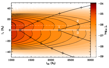
Figure 6: Part of the 6 cm synchrotron emission region, plotted as a function of $l_{\rm CD}$ (the length along the contact discontinuity) and $l_{\bot}$ (the distance from the contact discontinuity). The colour scale and contour lines indicate the value of the emissivity ($j_{\nu}$). The solid white line gives the position of the contact discontinuity and the shocks (which we assume to coincide). Positive $l_{\bot}$ values are oriented towards the primary. Because of the different physical conditions on either side of the contact discontinuity there is also a discontinuity in $j_{\nu}$. The dotted white line shows the offset of maximum emissivity from the shock (for the side towards the primary). For a selected number of points along the shock, we plot the tracks of the relativistic electrons as they are accelerated and advect out and cool down. These tracks are indicated by the black solid lines. The ‘+’ symbols on each track indicate one out of every 10 time steps we took. The positions indicated by the numbers $1-3$ are discussed in the text (Sect. 5.1.5).

A more detailed look at the emission (Fig. 6) reveals that most of the flux we detect is formed at some distance from the shock and must therefore be due to electrons that have cooled down somewhat. The figure shows the synchrotron emissivity $j_{\nu}$ in a coordinate system linked to the contact discontinuity. We limit the figure to distances of $1000-3000$ $R_{\sun}$, which is where most of the detectable radiation comes from.

Some care must be taken in the interpretation of this figure. The tracks show the particles to be moving away from the contact discontinuity/shock (which we assume to be at the same geometric position). This differs from the true hydrodynamical situation, where the particles move from the shock towards the contact discontinuity. This difference is a direct consequence of the simplifications in our model. It has a negligible influence, however, on the resulting fluxes and spectral index because the thickness of the synchrotron emitting region is quite small.

For a given point on the contact discontinuity (i.e., for a given $l_{\rm CD}$), the highest $j_{\nu}$ values are found at $l_{\bot}\approx 7-8\leavevmode\nobreak\ R_{\sun}$ from the shock (Fig. 6, dotted white line). The electrons responsible for this emission can be traced back to their acceleration point, which is some 300 $R_{\sun}$ earlier (in $l_{\rm CD}$). In addition to the strong $j_{\nu}$ changes orthogonal to the contact discontinuity, there is also a much weaker decreasing gradient as we move from the inside to the outside. In the flux calculation the outer regions get higher weight as this emissivity is rotated in to a three-dimensional volume.

To understand why the maximum is offset from the shock we simplify the situation by assuming that the electrons emit only at their maximum frequency and we concentrate on $p_{6}$, the characteristic momentum for 6 cm emission. At the shock at position ‘1’ (Fig. 6), a certain number density, $N_{1}(p_{6})$, of relativistic electrons is responsible for the 6 cm emission. Neglecting a weak function of $p_{\rm c}$, this number density is proportional to $\rho_{1}\Delta u_{1}^{2}$ (Eq. 8) with the subscript indicating the position. As these electrons advect out to position ‘2’, their number density decreases in proportion to $\rho$. Furthermore, while advecting, these electrons cool and therefore another set of electrons becomes responsible for the 6 cm emission. These are electrons that had $p>p_{6}$ at position ‘1’; their number density is less, so we introduce a factor $\epsilon$ ($<1$) to take that into account. At position ‘2’ their number density is $N_{2}(p_{6})$, which is proportional to $\epsilon\,\rho_{2}\Delta u_{1}^{2}$. Position ‘3’ is nearly the same as ‘2’, but it is on the shock. There, new relativistic electrons are generated with $N_{3}(p_{6})\propto\rho_{2}\Delta u_{3}^{2}$ (where we used $\rho_{2}\approx\rho_{3}$). Whether position ‘3’ or ‘2’ has the highest number density translates in to a comparison of $\rho_{2}\Delta u_{3}^{2}$ and $\epsilon\,\rho_{2}\Delta u_{1}^{2}$. The $\Delta u$ gradient is such that $\Delta u_{3}<\Delta u_{1}$ (Fig. 3, upper panel), so the result depends on whether the cooling is strong enough to overcome the effect of the $\Delta u$ gradient. The model calculations show that this is not the case and therefore $N_{2}>N_{3}$, resulting in a maximum emission that is offset from the shock. Only at large distances (beyond those shown on Fig. 6), does the compensating effect no longer work and there the models show the maximum to be at the shock. This, however, happens beyond the geometric region that contributes significantly to the observed radio flux.

It may seem surprising that the contribution of the outer regions of the wind is still detectable, considering that the energy going into the shock is small (as velocities are nearly tangential to the contact discontinuity). We can make a simple estimate to compare the inner and outer wind regions, based on the energy available from the shock. At a position $r$ along the contact discontinuity, we consider a section of length $\Delta r$. In a time interval $\Delta t$ a volume of material $2\pi r\,\Delta r\,\varv_{\bot}\Delta t$ crosses the shock through that section. The energy input rate is then: $1/2\;\rho\Delta u^{2}\,2\pi r\,\Delta r\,\varv_{\bot},$ of which a fraction $\zeta$ is used to accelerate the particles. The velocity orthogonal to the shock ($\varv_{\bot}$) is proportional to $r^{-1}$. We derive $\rho$ from the mass conservation equation in a spherically symmetric wind and approximate $\Delta u$ by $\varv_{\bot}$. If we assume that some constant fraction of the energy of accelerated particles goes into the synchrotron emission, we find that the radio luminosity of section $\Delta r$ is proportional to $\Delta r/r^{4}.$ An outer region of size $2000\leavevmode\nobreak\ R_{\sun}$ therefore contributes a fraction $10^{-3}$ of an inner region of size $200\leavevmode\nobreak\ R_{\sun}$. If we scale this to the calculated flux value of $\sim$ 700 mJy for the inner region (Fig. 5, middle column), we find 0.7 mJy for the outer region. None of the inner emission is detected due to the Razin effect and free-free absorption. The resulting flux is therefore predicted to be $\sim$ 0.7 mJy, which is consistent with the detailed models.

In summary, the standard model shows that phase-locked radio flux variability is indeed possible in Cyg OB2 No. 8A. The model fails however in predicting the phases of maximum/minimum flux and the spectral index.

5.2 An improved model

One possible approach to solve the problem with the phases of maximum/minimum flux is to “mirror-reverse” the system by exchanging the wind parameters of the primary and secondary star. It is important to realize that the star and wind parameters listed in Table 1 were not derived directly from information of the binary system, but rather from typical values for single stars with the same spectral type as the binary components. It is not clear how well such a procedure works for determining stellar parameters of binary components. This leads us to a more general approach, where we also explore models with star and/or wind parameters that are different from those listed in Table 1.

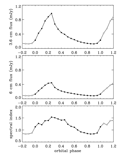
Figure 7: Results for the improved model plotted as a function of orbital phase. In this model the mass loss rate of the primary is $1.0\times 10^{-6}$ instead of $4.8\times 10^{-6}\,M_{\sun}\,{\rm yr}^{-1}$ and the terminal velocity is 2500 instead of 1873 ${\rm km\,s}^{-1}$. The upper panel shows the 3.6 cm flux, the middle panel the 6 cm flux and the lower panel the spectral index between those two wavelengths. As for Fig. 1, open symbols indicate duplications in the extended phase range.

In Fig. 7 we present one possible improved solution where we change the mass loss rate of the primary from $4.8\times 10^{-6}$ to $1.0\times 10^{-6}\,M_{\sun}\,{\rm yr}^{-1}$ and the terminal velocity from 1873 to 2500 ${\rm km\,s}^{-1}$. We present only this model from the large number of possibilities we explored, not because it presents a best-fit solution, but rather because it requires only minimal changes to the parameters compared to our standard model. Note that these changes result in the primary now having a weaker wind (less ram pressure) than the secondary.

We see in Fig. 7 that the phase of maximum is now 0.25, which is closer to the observed value (phase 0.1). Also the position of minimum flux at phase 0.9 (observed: 0.6) is improved compared to the standard model. The main reason for this is the change in shape of the contact discontinuity as can be seen in Fig. 8. The upper part of Fig. 8 shows the position of the contact discontinuity for the standard model. The observer looks from the bottom of the figure towards the top. We neglect in this discussion that the observer is not in the orbital plane, but 58° ($=90\degr-i$) above it. For the standard model we have maximum flux at phase 0.5 (Fig. 8, top left) because one arm of the contact discontinuity is then pointing in the direction of the observer and the star with the weaker wind (the secondary) is in front, so there is only a limited amount of absorption. At minimum (Fig. 8, top right) the contact discontinuity is well hidden by the stronger wind from the primary, which is in front.

The situation is quite different in the improved model. The secondary now has the stronger wind and therefore the contact discontinuity wraps around the primary. Maximum flux (Fig. 8, bottom left) again occurs when one arm of the contact discontinuity is pointing in the direction of the observer and the star with the weaker wind (primary) is in front, but this now happens at phase 0.25. At phase 0.5, the intrinsic synchrotron emission is even higher (see discussion Sect. 5.1.4), but the arm has rotated further along the orbit so that most of it is absorbed by the free-free absorption. At phase 0.9 (Fig. 8, bottom right) the contact discontinuity is hidden by the stronger wind from the secondary and therefore the flux is minimum.

Figure 8: Contact discontinuity of the standard model (top) and the improved model (bottom) plotted in the orbital plane. For both models, the configuration is shown for maximum (left) and minimum (right) flux. Also indicated are the primary and secondary stars, as well as the binary orbit (assumed centred on the primary). The observer looks from the bottom of the page towards the top.

Although the phases of minimum and maximum are now closer to their observed values, the agreement is still not very good. However, the present model does not take into account the effect of orbital motion. The importance of this effect is shown by, e.g. Pittard (2009). In the specific case of Cyg OB2 No. 8A, we have significant emission coming from $10-30$ times the binary separation; orbital effects at these distances will definitely play a role. Because of the orbital motion, the contact discontinuity will get distorted resulting in a leading arm that is further from the strong-wind secondary than the trailing arm. This will shift the phases at which minimum and maximum occur. Consider, e.g. maximum flux, where the part of the contact discontinuity closest to the observer is pointing in the direction of the observer (phase 0.25 in Fig. 8, bottom left). Including orbital motion will push this further away along the orbit from the strong-wind secondary. In order to have the contact discontinuity pointing again in the direction of the observer, we need to move the secondary back somewhat in its orbit. Maximum flux will thus occur at an earlier phase. Including orbital motion will therefore result in a better agreement with the observed phases of maximum and minimum flux.

One remaining problem is the spectral index, which is still considerably different from the observed value of $\sim$ 0.0. The spectral index is the result of the combined influence of free-free absorption and the Razin effect. As we saw in Sect. 5.1.4, the spectral index is highly sensitive to the value of the thermal electron density $n_{\rm e}$, through the Razin effect. The physical basis of this effect is that the local thermal electrons result in a refraction index which changes the relativistic beaming of the synchrotron radiation thereby reducing the emitted power (Ginzburg & Syrovatskii 1965). In Sect. 5.1.5 we showed that introducing free-free absorption changes the spectral index as well.

In order to model the observed spectral index, the simplest possibility is to reduce the mass-loss rates of the stars. The reduced density will result in both less free-free absorption and a reduction of the Razin effect. As synchrotron emissivity is proportional to $n_{\rm e}$ this suggests that the flux would go down. But this is easily compensated for by the flux increase due to the reduction of the Razin effect, as a comparison of Fig. 4 middle and right columns shows. In order to be consistent with observations of single stars, such a reduced-density wind will need to be clumped (e.g. Puls et al. 2008). This would complicate the proposed explanation: the clumping would again increase the free-free absorption, probably to levels comparable to that of a smooth high-density wind. This, in turn, could be counteracted by the destruction of clumps in colliding-wind binaries (Pittard 2007). Another possibility is the effect of porosity (Shaviv 1998; Owocki & Cohen 2006), where at least some of the clumps are optically thick thereby allowing more radiation to escape through the inter-clump medium. A further effect is that hot, low-density regions may persist even in the radiative part of the colliding-wind region (especially on the leading edge of each arm, Pittard 2009). The low density will reduce the Razin and free-free effects, resulting in a spectral index closer to the observations.

We also recall that, in our model, we left out the free-free absorption and emission due to the density and temperature changes in the colliding-wind region. Pittard (2010) presents models that study this effect. His Fig. 14 shows that the free-free contribution from the colliding-wind region has an intrinsic spectral index which can be close to 0. However, including the free-free contribution of the winds results in a positive index. This therefore does not help in explaining the observed spectral index.

Figure 9: Contact discontinuity of the standard model (top) and the improved model (bottom) plotted in the orbital plane. For both models, the configuration is shown for periastron (left) and apastron (right). Primary and secondary star, and binary orbit are as indicated in Fig. 8. The dotted line shows the sight-line from the observer to the apex of the contact discontinuity.

5.3 X-ray emission

In Sect. 3, we noted the anti-correlated behaviour of the X-ray and radio light curves. The observed X-ray flux is caused by thermal emission due to heating in the wind-collision zone and subsequent absorption in the stellar wind material. Both the heating and the absorption change with stellar phase and thus lead to variability, just as for the radio fluxes. But the difference with the radio emission is that the optical depths are very much smaller in X-rays. For single stars, thermal X-ray emission that is formed in shocks due to the radiative driving instability can be seen down to $1-2$ stellar radii (Kramer et al. 2003). Radio emission, on the other hand, can only be seen from $\sim 100$  stellar radii. In a massive colliding-wind binary such as Cyg OB2 No. 8A this means that the radio emission will come from outer parts of the contact discontinuity, but the X-ray emission will be formed close to the apex of the contact discontinuity.

Minimum flux occurs at periastron in this eccentric binary, where the distance between the two components is smallest. The winds have attained only a fraction of their terminal velocities before colliding, resulting in a lower post-shock temperature. In addition, with the reduced separation, the X-ray emitting plasma is buried in denser wind material. This leads to a stronger absorption of the X-rays emitted by the plasma heated by the colliding winds, which is clearly seen in the measured local absorption column densities (Fig. 2, upper panel). This results in a strong decrease of the emerging X-ray flux at this orbital phase, even though an increase of intrinsic X-ray flux (that scales with the emission measure) is expected. At apastron, the winds have higher velocities before colliding, resulting in a higher post-shock temperature, but the absorption by the wind material surrounding the apex of the wind interaction region (where the bulk of the X-rays are produced) is significantly reduced. The global shape of the X-ray light curve results in fact from the combined effect of varying post-shock temperature as a function of the separation, changing photoelectric absorption along the line of sight, and decreasing emission measure when going from periastron to apastron.

When we replace the standard model by the improved one, the contact discontinuity now wraps around the primary rather than the secondary. This changes the absolute position of the apex, but not the relative behaviour of the X-ray emission measure as a function of orbital phase. Phases of minimum and maximum emission measure will be the same for the two models.

Fig. 2 (upper panel) shows that the observed absorption column changes with orbital phase. This puts an additional constraint on the models. To see if our modelling is qualitatively consistent with this, we consider the sight-line of the observer toward the apex (Fig. 9) and we discuss the absorption column along that line. At periastron (phase 0.0) in the standard model, the sight-line passes through the stronger wind while at apastron (phase 0.5) it passes through the weaker wind. Because of the position of the apex, the sight-line also passes closer to the star at periastron than at apastron (Fig. 9, upper panel). One should also take into account that the sight-line is not in the plane of the orbit, but at an angle of 58° ($=90\degr-i$) above it. For the standard model, maximum absorption therefore occurs near periastron, minimum absorption near apastron, which is consistent with the observed behaviour shown in Fig. 2 (upper panel). For the improved model, on the contrary, the sight-line goes through the weaker wind at periastron. This might suggest a reversal of the phases for minimum and maximum absorption. However, the dominant effect is how close the sight-line passes to the relevant star. Fig. 9 (lower panel) clearly shows that this still occurs at periastron. Both the standard and improved model are therefore qualitatively in agreement with the observed behaviour of the absorption column.

Pittard & Parkin (2010) present models for the thermal X-ray emission in O+O star binaries. They discuss Cyg OB2 No. 8A, although no specific model for this system is presented. One of their models is an eccentric binary which has a light curve qualitatively similar to the lower panel in Fig. 1: it shows a roughly constant flux for a large part of the orbit, followed by a rather sharp maximum which in turn is followed by the minimum. Also their model predicts changes in the hottest component of the emission, which is indeed observed, though caution should be used in the interpretation of this result as the error bars are quite large (see Sect. 3).

5.4 Future work

The improved model presented here is qualitatively successful in explaining a number of important features of the radio emission of the colliding-wind binary Cyg OB2 No. 8A. Nevertheless, it should be realized that some important physical ingredients are still missing. The major ones are including orbital motion and solving the equations of hydrodynamics. Orbital motion will have an important effect on the phases of minimum and maximum flux. Solving the hydrodynamics equations will allow us to correctly position the shocks and take into account the instabilities and inhomogeneities, as they influence both the thermal free-free emission and absorption, and the synchrotron emission. Information from hydrodynamics will also allow us to replace the assumed shock strength $\chi=4$ by its correct value. This will influence the relativistic electron momentum distribution. In addition, clumps that are optically thick at radio wavelengths will result in porosity, letting a larger fraction of the synchrotron emission escape. Finally, future models should handle both the X-ray and radio emission simultaneously, giving us a consistent picture of these colliding-wind systems.

6 Conclusions

We determined the radio light curve of Cyg OB2 No. 8A, based on new and archive VLA observations. We find phase-locked variability in the radio fluxes. This is contrary to expectations, as the synchrotron emission due to the colliding winds should be hidden by free-free absorption in this close binary. We also present an updated version of the X-ray light curve. The radio and X-ray light curves are nearly anti-correlated, which is another unexpected result.

Our model calculation for the radio flux shows that the synchrotron emission region extends considerably beyond the apex of the colliding-wind region, explaining why we do see phase-locked variability. We achieve this result without any need for clumping or porosity in the model. Our standard model – which uses the star and wind parameters proposed by De Becker et al. (2006) – does not correctly predict the phases of minimum and maximum. When we change the wind parameters (which are not well-determined) to make the secondary have the stronger wind, we find a considerable improvement in phases of minimum/maximum. A more detailed study of Cyg OB2 No. 8A is therefore needed to better determine the star and wind parameters of its binary components. To improve the phase agreement even further we will need to include orbital motion in the model.

The nearly anti-correlated behaviour of the X-ray and radio light curves is due to their very different formation regions. X-rays are formed quite close to the apex of the contact discontinuity, where the heating is strongest and they suffer only a limited amount of absorption. Radio emission, on the other hand, is strongly absorbed, so the radio emission we can detect is formed much further out along the contact discontinuity. Because the contact discontinuity is curved, this results in X-rays and radio having their minimum/maximum flux at very different phases.

The model values for the radio spectral index (+0.75 to +1.5) differ considerably from the observed value of $\sim$ 0.0. However, the model values are quite sensitive to the density of the thermal electrons, which are responsible for the Razin effect and the free-free absorption. A decrease of that density would allow a better agreement with the observations. Such a decrease could be due to lower density regions caused by hydrodynamical effects in the colliding-wind region or by clumping in a wind with a reduced mass-loss rate. Although we did not require clumping or porosity to explain the phase-locked variability, it is likely that we will need it to explain the observed spectral index. Because of the high sensitivity of the spectral index to clumping conditions, it could provide a valuable pathway to investigate the well-known problem of clumping in single-star winds. Future, improved models, applied to Cyg OB2 No. 8A and other non-thermal radio emitters should therefore be capable of determining limits on this clumping.

Appendix A Modelling

Most of the calculations discussed here are limited to the two-dimensional (2D) plane of the binary orbit. Only in Sect. A.7 do we rotate the results of the 2D calculations into the three-dimensional (3D) simulation volume that is used to calculate the resulting flux.

A.1 Binary orbit

Figure 10 shows how the two stars are positioned in the XY plane of the 3D simulation volume. The primary is at the centre of the volume and the position of the secondary is determined by the orbital phase. The angle of periastron ($\omega$) is measured from the intersection of the plane of the sky with the plane of the orbit. The sight-line towards the observer is in the YZ plane and the inclination angle $i$ is the angle between the plane of the sky and the orbital plane. The secondary rotates clockwise in this figure (as seen from above). Periastron corresponds to phase 0.0.

Figure 10: Binary orbit in the XY plane of the 3D simulation volume. The primary is positioned at the centre of the volume. The argument of periastron is denoted $\omega$ and the inclination angle $i$. The units on the axes are $R_{\sun}$.

A.2 Contact discontinuity

The position of the contact discontinuity at any given orbital phase is determined by the balance of ram pressure between the velocity components orthogonal to the contact discontinuity (see equations in Antokhin et al. 2004). These equations take into account that the terminal velocity of the winds may not have been reached yet before they collide. Specifically, in the Cyg OB2 No. 8A standard model presented in Sect. 5.1, the winds collide with $0.65\,\varv_{\infty}$ (primary) and $0.71\,\varv_{\infty}$ (secondary) at the apex at periastron. After the stellar wind material has passed through the shock, it then moves outward parallel to the contact discontinuity (there is also a small orthogonal velocity component, see Sect. A.5). We assume that the shocks and the contact discontinuity are sufficiently close to one another that we do not need to make a distinction in their geometric positions. On each side of the contact discontinuity, we assume the stellar wind to have a $\beta=1$ velocity law and a density derived from the mass conservation law, using the assumed velocity law and mass-loss rate.

A.3 Momentum distribution relativistic electrons

We determine the momentum distribution of the relativistic electrons for a grid of points along the two shocks. We start with a population of electrons generated at a given point on the shock itself. We then follow the time evolution of this population as it advects away and cools down. The momentum distribution uses a grid that is uniform in $\log p$, between $p_{0}=1.0$ MeV/$c$ (for the choice of this specific value, see Van Loo et al. (2004)) and the upper limit $p_{\rm c}$ (defined below, Eq. 5) These limits are sufficiently wide to cover all of the radio emission we are interested in. We stop following the electrons when their momentum falls below $p_{0}$, or when they leave the simulation volume. (In our calculations we checked that the emission beyond the simulation volume is negligible.)

In the following, we refer mainly to Van Loo (2005, hereafter VL) as the source for the equations. Citations to the original papers can be found in that reference.

A.4 New relativistic electrons

At the shock, new relativistic electrons are put into the system. Taking into account the particle acceleration mechanism and the inverse Compton cooling, it can be shown that their momenta follow a modified power-law distribution ( VL, Eqs. 5.5, 5.6):

$$N(p) = N_{\rm E}p^{-n}\left(1-\frac{p^{2}}{p_{\rm c}^{2}}\right)^{(n-3)/2},$$ (3)

$$n = \frac{\chi+2}{\chi-1}.$$ (4)

With ( VL, Eqs. 5.1-3):

$$\left(\frac{p_{\rm c}}{m_{\rm e}c}\right)^{2}=\frac{\chi\Delta u^{2}}{\chi^{2}-1}\frac{4\pi r^{2}}{\sigma_{\rm T}L_{*}}\frac{eB(r)}{c},$$ (5)

with $m_{\rm e}$ and $e$ the mass and charge of the electron, $\sigma_{\rm T}$ the Thomson electron scattering cross section, $c$ the speed of light, $L_{*}$ the luminosity of the star and $r$ the distance of the point on the shock to the star. Because there are two stars, we should calculate the contribution of both:

$$\frac{L_{*}}{r^{2}}=\frac{L_{*,1}}{r_{1}^{2}}+\frac{L_{*,2}}{r_{2}^{2}},$$ (6)

with $r_{1}$ the distance to the primary and $r_{2}$ the distance to the secondary. Also ( VL, Eq. 3.7):

$$\Delta u=u_{1}-u_{2}=u_{1}\frac{\chi-1}{\chi},$$ (7)

where $u_{1}$ is the upstream velocity and $u_{2}$ the downstream one and the shock strength $\chi=u_{1}/u_{2}$. Throughout this work we assume strong shocks with $\chi=4$, but we note that higher values can be expected in radiative shocks.

The normalization factor $N_{\rm E}$ is related to $\zeta$, the fraction of energy that gets transferred from the shock to the relativistic particles, by ( VL, Eq. 5.10):

$$N_{\rm E}=4\frac{\zeta}{\displaystyle\log_{\rm e}\left(\frac{p_{\rm c}}{p_{0}}\right)}\rho_{1}\frac{\Delta u^{2}}{c}\quad({\rm for}\leavevmode\nobreak\ \chi=4),$$ (8)

where $\rho_{1}$ is the upstream density and we assume $\zeta=0.05$ (Blandford & Eichler 1987; Eichler & Usov 1993).

The magnetic field at distance $r$ to the relevant star is assumed to be given by (Weber & Davis 1967; VL Eq. 2.48):

$$B(r)=B_{*}\frac{\varv_{\rm rot}}{\varv_{\infty}}\frac{R_{*}}{r},$$ (9)

where $B_{*}$ is the surface magnetic field (assumed to be 100 G) and $\varv_{\rm rot}$ is the equatorial rotational velocity. This equation is only valid at larger distances from the star, but we use it everywhere as the region close to the star will not be visible anyway (due to free-free absorption). This equation neglects any amplification of the field (such as described by, e.g. Bell (2004)) or any reduction by magnetic reconnection. For each of the two shocks, the corresponding magnetic field is taken into account.

A.5 Advection and cooling

During a time step $\Delta t$, the relativistic electrons advect away and cool mainly due to inverse Compton and adiabatic cooling (see Chen (1992) and VL (p. 96) for a discussion on other cooling mechanisms and why they are not important in the present situation).

The equation for cooling of a single relativistic electron can be written as:

$$\frac{{\rm d}p}{{\rm d}t} = -ap^{2}+bp\quad\mbox{with}$$ (10)

$$a = \frac{\sigma_{\rm T}}{3\pi m_{\rm e}^{2}c^{3}}\frac{L_{*}}{r^{2}},$$ (11)

$$b = \frac{1}{3\rho}\frac{\Delta\rho}{\Delta t},$$ (12)

where $ap^{2}$ gives the inverse Compton cooling ( VL, Eq. 5.2) and $bp$ the adiabatic cooling (which can be derived from the fact that for adiabatic cooling $p\propto T^{1/2}\propto\rho^{(\gamma-1)/2}$ and using $\gamma=5/3$).

Integration of Eq. 10 gives:

$$p=\frac{p_{\rm init}\exp(b\Delta t)}{\displaystyle 1-\frac{a}{b}p_{\rm init}\left(1-\exp(b\Delta t)\right)},$$ (13)

where $p_{\rm init}$ is the momentum at the previous time step. We can invert this to:

$$p_{\rm init}=\frac{p\exp(-b\Delta t)}{\displaystyle 1-\frac{a}{b}p\left(1-\exp(-b\Delta t)\right)}.$$ (14)

We will also need the following derivative:

$$\frac{{\rm d}p_{\rm init}}{{\rm d}p}=\frac{\exp(-b\Delta t)}{\displaystyle\left[1-\frac{a}{b}p\left(1-\exp(-b\Delta t)\right)\right]^{2}}.$$ (15)

We assume that only the momentum $p$ changes significantly with time; for the other variables, we take their value mid-way between the start and the end of the time step $\Delta t$. The density $\rho$ we need in Eq. 12 is the one between the shock and the contact discontinuity. We do not have detailed hydrodynamical models for this, so we simply approximate it by $\rho=\chi\rho_{\rm s}$ where $\rho_{\rm s}$ is the density in the smooth wind at the position of the shock. We stress once again that in these radiative shocks, the post-shock density increases rapidly downstream, maybe by several orders of magnitude, rather than the $\chi=4$ value we use.

The above equations describe what happens to a single relativistic electron. The time evolution of the momentum distribution function over the time step $\Delta t$ is:

$$N(p)=N(p_{\rm init})\frac{\rho(t+\Delta t)}{\rho(t)}\frac{{\rm d}p_{\rm init}}{{\rm d}p}.$$ (16)

We stop following the electrons when their momentum falls below $p_{0}$, or when they leave the simulation volume.

In our simplifying assumptions the contact discontinuity and the shock are at the same geometrical position. Taken literally, this would result in a synchrotron emitting region that has zero thickness and zero synchrotron emission. In the true hydrodynamical situation, particles move through the shock (which is at some distance from the contact discontinuity) and then move slowly towards the contact discontinuity. At the same time, they are being advected outward with a velocity parallel to the contact discontinuity that is much larger than the corresponding orthogonal velocity. The thickness of the synchrotron emitting region is set by the combination of these two velocities. In the absence of hydrodynamical information, we use the following procedure to determine these velocities. The parallel component ($\varv_{\|}$) at the contact discontinuity is determined by projecting the smooth wind velocity vector on to the contact discontinuity. At other positions in the wind, we interpolate in the grid of $\varv_{\|}$ as a function of the y-coordinate. The orthogonal component ($\varv_{\bot}$) at the contact discontinuity is expected to be of the order of the orthogonal component of the material coming into the shock, with a minimum value corresponding to the thermal expansion of the gas. As a simplification, we set it exactly equal to the incoming orthogonal component, and we use the same type of interpolation as for the parallel velocity to determine it at other positions. We reverse the orthogonal velocity direction to have the gas moving away from the contact discontinuity. Note that this situation is “inside out” compared to the true hydrodynamical situation where the particles move towards the contact discontinuity. The thickness of the synchrotron emitting region is so small however that this inversion has negligible influence on our results.

A.6 Emissivity

The equation for the emissivity is given by ( VL, Eq. B.1):

$$j_{\nu}(r) = \frac{1}{4\pi}\int_{p_{0}}^{p_{\rm c}}{\rm d}pN(p,r)\int_{0}^{\pi}\frac{{\rm d}\theta}{4\pi}2\pi\sin\theta\frac{\sqrt{3}e^{3}}{m_{\rm e}c^{2}}$$ (17)

$$\quad\quad\quad Bf(\nu,p)\sin\theta F\left(\frac{\nu}{f^{3}(\nu,p)\nu_{\rm s}(p,r)\sin\theta}\right),$$

With ( VL, Eq. 2.51, 2.50):

$$f(\nu,p) = \left[1+\frac{\nu_{0}^{2}}{\nu^{2}}\left(\frac{p}{m_{\rm e}c}\right)^{2}\right]^{-1/2}$$ (18)

$$\nu_{0} = \sqrt{\frac{n_{\rm e}e^{2}}{\pi m_{\rm e}}}$$ (19)

$$\nu_{\rm s}(p,r) = \frac{3}{4\pi}\frac{eB}{m_{\rm e}c}\left(\frac{p}{m_{\rm e}c}\right)^{2}$$ (20)

$$F(x) = \int_{x}^{\infty}{\rm d}\eta K_{5/3}(\eta).$$ (21)

We use Eq. 9 for the magnetic field. Note that this is an approximation, as the shock may compress the magnetic field as well, leading to higher values than given by Eq. 9. The expression for $j_{\nu}(r)$ is evaluated at position $r$ and frequency $\nu$. The $f$ function corrects for the Razin effect and $K_{5/3}$ is the modified Bessel function. To calculate $n_{\rm e}$, the number density of the thermal electrons (i.e. those in the non-relativistic plasma), we use:

$$n_{\rm e}=\frac{\chi\rho_{\rm s}}{m_{\rm H}}\frac{1.2}{1.4},$$ (22)

where $\rho_{\rm s}$ is the smooth wind density and $m_{\rm H}$ the mass of a hydrogen atom. The factor 1.2/1.4 takes into account a fully ionized hydrogen+helium solar composition. In these radiative shocks the post-shock density may increase by several orders of magnitude rather than by $\chi=4$, which will influence the value of $n_{\rm e}$.

To reduce the computing time we set $\sin\theta=1$ in the $f\sin\theta$ factors of Eq. 17 and we also use:

$$\int_{0}^{\pi}\frac{{\rm d}\theta}{4\pi}{2\pi\sin\theta}=1.$$ (23)

The $F$ function is precalculated on a grid of $x$-values; the evaluation of the function then reduces to an interpolation.

A.7 Map into 3D grid

Using the equations from the previous sections, we can make a 2D map of the synchrotron emission (part of which is shown in Fig. 6). Note that the synchrotron emission extends on both sides of the contact discontinuity, because there is a shock on either side. Based on the cylindrical symmetry around the line connecting the two stars (at the given orbital phase), we then “rotate” this 2D map into the 3D simulation volume.

It is important that during this procedure we do not lose part of the emission due to interpolation or reduced resolution. To achieve this, we use volume-integrated emissivities. While doing the 2D calculation we store the volume integrated emissivity $\overline{j_{\nu}(r)}$ defined by:

$$\overline{j_{\nu}(r)}\Delta V=\int_{\Delta V}j_{\nu}(r){\rm d}V.$$ (24)

The volume $\Delta V$ used in this definition is determined as follows. We consider the 2D surface covered by (1) the step in the coordinate along the contact discontinuity and (2) the distance travelled by the relativistic electrons between two consecutive time steps. We then rotate this surface around the line connecting the two stars over a small angle $\alpha$, thereby defining the emissivity volume $\Delta V$.

When we have finished the full 2D calculation, we rotate the 2D plane into the 3D simulation volume, using steps of angle $\alpha$ (as defined above). For each of the emissivity volumes $\Delta V$ defined above, and for a given rotation angle, we determine what fraction of the rotated volume overlaps with the cells in the 3D simulation volume. This is done by subdividing each dimension of the $\Delta V$ volume into three. For each of the resulting $3^{3}$ points we determine in which 3D simulation cell they end up after rotation. A running sum for that cell is then updated with the fraction $3^{-3}$ of the volume integrated emissivity $\overline{j_{\nu}}$ of the rotated volume. At the end of this procedure, the accumulated emission in each 3D simulation cell is divided by its volume, thus obtaining $j_{\nu}$ for that cell.

In this procedure we lose some resolution, specifically around the apex, where the 2D resolution is quite high but where the 3D resolution is much lower. However, because of the use of volume-integrated quantities, we do not lose any of the synchrotron emission. Furthermore, the apex of the wind is well hidden by the free-free absorption and will therefore not contribute to the resulting radio flux at the wavelengths we consider. If our model were to be applied to X-rays, optical emission or radio emission at much shorter wavelengths, a higher-resolution 3D grid would be required.

In the 3D model. we also include the thermal free-free opacity and emissivity, which is due to the ionized wind material. To calculate these we use the Wright & Barlow (1975) equations. The winds of both stars are assumed to be smooth. For the Gaunt factor at frequency $\nu$ we use the equation from Leitherer & Robert (1991):

$$g_{\nu}=9.77\left(1+0.13\log_{10}\frac{T_{\rm e}^{3/2}}{Z\nu}\right),$$ (25)

where $T_{\rm e}$ is the thermal electron temperature in the wind and $Z$ the charge of the ions. The stars themselves are introduced into the simulation volume as high opacity spheres. We then solve the radiative transfer equation in Cartesian coordinates along the line of sight. We use Adam’s (Adam 1990) finite volume method because of its simplicity. By repeating the whole procedure for a number of orbital phases and wavelengths, we calculate the radio light curve at these wavelengths and determine how the fluxes and spectral index change with phase.

Appendix B Data reduction

The data reduction is accomplished using the Astronomical Image Processing System (AIPS), developed by the NRAO. We follow the standard procedures of antenna gain calibration, absolute flux calibration, imaging and deconvolution. Where possible, we apply self-calibration to the observations (see notes to Table B). We measure the fluxes and error bars by fitting elliptical Gaussians to the sources on the images. The error bars listed in Table B include not only the rms noise in the map, but also an estimate of the systematic errors that were evaluated using a jackknife technique. This technique drops part of the observed data and redetermines the fluxes, giving some indication of systematic errors that can be present. Upper limits are three times the uncertainty as derived above. For details of the reduction, we refer to the previous papers in this series (Blomme et al. 2005, 2007; Van Loo et al. 2008). We exclude from Table B those observations with upper limits higher than 6 mJy (which corresponds to about 3 times the highest detection at all wavelengths).

A comparison with values previously published in the literature shows that in most cases the error bars overlap with ours. There are just a few exceptions, which we discuss further. Bieging et al. (1989) list only an upper limit for the AC116 2 cm observation, while we find a detection (though marginal at just above 3 sigma). Our detection is quite consistent in all variants we consider in the jackknife test and is at the exact position of Cyg OB2 No. 8A, so we consider it a detection. For the AS483 6 cm, Waldron et al. (1998) find a value of 1.04 $\pm$ 0.08 mJy, which is $\sim$ 20% lower than our value. A possible explanation is that they did not correct for the decreasing sensitivity of the primary beam. This effect is important when the target is not in the centre of the image, and is approximately 20% for the position of No. 8A on the image. Puls et al. (2006) list an upper limit of 0.54 mJy for the AS786 6 cm observation, but we clearly detect Cyg OB2 No. 8A on the image we made. Bieging et al. (1989) find a slightly lower value of 1.0 $\pm$ 0.1 mJy for the AC116 1984-12-21, 20 cm observation. We have no explanation for these last two discrepancies.

We also take the opportunity to correct some clerical errors in the literature: Bieging et al. (1989) date the CHUR observations as 1980-Mar-22, but it should be 1980-May-23. The Waldron et al. (1998) 1991 observation was made at 3.6 cm, not at 6 cm and the 1992 observation was made in January, not June.

[x]lllrrcrrrlcl Reduction of the Cyg OB2 No. 8A VLA data.
(1) (2) (3) (4) (5) (6) (7) (8) (9) (10) (11)
Progr. Date Ctr. Phase Calibrator Int. No. Config. Flux Notes
Name Flux Dist. Time Ants.
(Jy) (degr.) (min) (mJy)
continued.
(1) (2) (3) (4) (5) (6) (7) (8) (9) (10) (11)
Progr. Date Ctr. Phase Calibrator Int. No. Config. Flux Notes
Name Flux Dist. Time Ants.
(Jy) (degr.) (min) (mJy)
2 cm
AA28 1984-03-04 8 2007+404 3.33 $\pm$ 0.28 4.9 20 27 CnB 0.7 $\pm$ 0.4
AC116 1984-12-21 8 2007+404 3.96 $\pm$ 0.07 4.9 10 27 A 0.62 $\pm$ 0.19
AS786 2004-02-15 7 2015+371 2.88 $\pm$ 0.03 5.4 60 26 CnB $<$ 4.
3.6 cm
AS397 1990-02-16 8 2007+404 3.10 $\pm$ 0.04 4.9 59 22 A 0.48 $\pm$ 0.05
AH395 1990-02-17 8 2007+404 3.05 $\pm$ 0.01 4.9 44 22 A 0.66 $\pm$ 0.04
AW288 1991-07-04 8 2025+337 2.08 $\pm$ 0.06 7.7 5 26 A 0.70 $\pm$ 0.09
AW304 1992-01-24 8 2007+404 2.87 $\pm$ 0.03 4.9 12 24 CnB 1.06 $\pm$ 0.07 S
BP1 1992-05-30 9 2052+365 1.87 $\pm$ 0.01 6.0 99 23 DnC $<$ 1.1
AB671 1993-01-24 9 2007+404 3.33 $\pm$ 0.07 4.9 23 27 A $<$ 5. S
AB671 1993-01-29 9 2007+404 3.33 $\pm$ 0.02 4.9 24 27 BnA $<$ 2.0 S
AB671 1993-02-01 9 2007+404 3.29 $\pm$ 0.03 4.9 6 27 BnA $<$ 4.
AB671 1993-02-14 9 2007+404 3.41 $\pm$ 0.03 4.9 7 27 BnA $<$ 4. S
AB671 1993-02-20 9 2007+404 3.8 $\pm$ 0.1 4.9 14 24 B $<$ 5.
AS483 1993-05-01 98 2007+404 3.28 $\pm$ 0.01 4.9 25 27 B 1.19 $\pm$ 0.13 S
AR277 1994-04-17 9 2007+404 2.97 $\pm$ 0.01 4.9 23 14 A $<$ 5. S
AR328 1995-04-27 9 2007+404 2.77 $\pm$ 0.01 4.9 11 16 D $<$ 2.7
AS644 1999-02-05 7 2007+404 2.07 $\pm$ 0.12 4.9 35 23 DnC 1.0 $\pm$ 0.3
AS644 1999-04-18 8 2015+371 2.17 $\pm$ 0.01 4.9 5 27 D 0.92 $\pm$ 0.10
AW515 1999-06-08 9 2007+404 2.02 $\pm$ 0.01 4.9 10 19 AD $<$ 2.8 I,S
BB116 1999-12-04 9 2007+404 2.20 $\pm$ 0.01 4.9 101 27 B 1.96 $\pm$ 0.26
BB116 2000-06-26 9 2007+404 2.40 $\pm$ 0.01 4.9 20 26 DnC 2.9 $\pm$ 2.3
AS786 2004-02-15 7 2015+371 2.76 $\pm$ 0.02 5.4 45 25 CnB 1.12 $\pm$ 0.18
BD110 2005-11-15 9 2007+404 2.29 $\pm$ 0.02 4.9 21 22 D $<$ 2.1 S
AB1195 2006-01-26 8 2007+404 2.37 $\pm$ 0.05 4.9 31 16 AD 0.58 $\pm$ 0.27
AB1210 2006-05-24 8 2007+404 2.21 $\pm$ 0.02 4.9 27 21 BnA 0.98 $\pm$ 0.05
6 cm
CHUR 1980-05-23 8 2007+404 4.73 $\pm$ 0.03 4.9 47 22 AD 1.33 $\pm$ 0.13 1x50
CHUR 1980-05-24 8 2007+404 4.58 $\pm$ 0.03 4.9 47 22 AD 1.18 $\pm$ 0.11 1x50
BIGN 1981-10-16 9 2007+404 4.16 $\pm$ 0.04 4.9 17 27 C 0.8 $\pm$ 0.4 S,1x50
BECK 1982-03-27 9 2007+404 4.74 $\pm$ 0.01 4.9 228 27 A 1.5 $\pm$ 0.4 S,1x50
BECK 1982-07-03 9 2007+404 4.95 $\pm$ 0.02 4.9 5 26 A $<$ 5. S,1x50
BIEG 1982-08-26 9 2007+404 4.4 $\pm$ 0.1 4.9 9 24 B $<$ 3. 1x50
BECK 1982-12-21 9 2023+318 2.86 $\pm$ 0.01 9.6 9 24 D $<$ 2.4 S,1x50
AC42 1983-05-09 9 2007+404 4.46 $\pm$ 0.02 4.9 10 26 C $<$ 1.2 1x50
AC42 1983-08-22 9 2007+404 4.85 $\pm$ 0.01 4.9 14 25 A $<$ 4.
AB228 1983-08-27 9 2007+404 4.90 $\pm$ 0.03 4.9 18 27 A $<$ 3.
AB252 1983-10-30 9 2007+404 4.84 $\pm$ 0.02 4.9 9 26 A $<$ 4. S
AA28 1984-03-04 8 2007+404 4.27 $\pm$ 0.01 4.9 41 27 CnB 0.91 $\pm$ 0.10
AA28 1984-03-09 8 2007+404 4.33 $\pm$ 0.01 4.9 23 26 CnB 0.78 $\pm$ 0.13
AA29 1984-04-04 9 2007+404 4.21 $\pm$ 0.02 4.9 11 27 C $<$ 0.9 S
VM59 1984-10-16 9 2202+422 2.72 $\pm$ 0.01 16.7 13 26 D $<$ 2.4 S
AC116 1984-11-27 9 2007+404 4.50 $\pm$ 0.01 4.9 19 25 A $<$ 2.8 S
AC116 1984-12-21 8 2007+404 4.63 $\pm$ 0.01 4.9 6 27 A 0.56 $\pm$ 0.13
AF102 1985-05-09 + 2022+616 2.43 $\pm$ 0.01 20.4 9 26 B $<$ 1.3 S
AA47 1985-06-12 7 2007+404 3.87 $\pm$ 0.01 4.9 24 22 B 0.98 $\pm$ 0.27
AA47 1985-09-01 9 2007+404 3.53 $\pm$ 0.01 4.9 7 27 C $<$ 1.0
AA47 1985-09-19 9 2007+404 3.56 $\pm$ 0.01 4.9 11 25 C $<$ 0.8
VM115 1990-06-11 9 2202+422 3.24 $\pm$ 0.01 16.7 19 22 A $<$ 1.6
AG320 1991-03-06 SE 2007+404 2.73 $\pm$ 0.01 5.3 10 25 D 1.4 $\pm$ 0.6
AB671 1993-01-21 9 2007+404 3.09 $\pm$ 0.01 4.9 19 24 A $<$ 2.3 S
AB671 1993-01-24 9 2007+404 3.08 $\pm$ 0.03 4.9 18 27 A $<$ 2.8 S
AB671 1993-01-29 9 2007+404 3.12 $\pm$ 0.02 4.9 19 27 BnA 2.1 $\pm$ 1.1 S
AB671 1993-02-01 9 2007+404 3.11 $\pm$ 0.01 4.9 7 27 BnA 1.2 $\pm$ 0.7 S
AB671 1993-02-14 9 2007+404 3.12 $\pm$ 0.02 4.9 8 27 BnA 2.2 $\pm$ 1.4
AS483 1993-05-01 98 2007+404 3.04 $\pm$ 0.01 4.9 21 25 B 1.33 $\pm$ 0.16
TST6CM 1993-06-04 9 2052+365 5.2 $\pm$ 0.2 6.0 29 26 CnB $<$ 0.8 X
AR277 1994-04-17 9 2007+404 3.04 $\pm$ 0.01 4.9 23 15 A $<$ 4.
AR328 1995-04-27 9 2007+404 2.982 $\pm$ 0.003 4.9 11 16 D $<$ 2.3
AS644 1999-02-05 7 2007+404 2.6 $\pm$ 0.1 4.9 20 23 DnC 1.1 $\pm$ 0.5
AS644 1999-04-18 8 2015+371 1.728 $\pm$ 0.003 5.4 5 26 D 0.93 $\pm$ 0.19
AW515 1999-06-08 9 2007+404 2.40 $\pm$ 0.03 4.9 10 21 AD $<$ 1.4 I,S
AS786 2004-02-15 7 2015+371 2.778 $\pm$ 0.003 5.4 61 26 CnB 1.21 $\pm$ 0.28
AB1156 2005-02-04 8 2007+404 2.47 $\pm$ 0.01 4.9 31 25 BnA 1.28 $\pm$ 0.05
AB1156 2005-02-06 8 2007+404 2.50 $\pm$ 0.02 4.9 31 25 BnA 1.27 $\pm$ 0.06
AB1156 2005-02-08 8 2007+404 2.52 $\pm$ 0.01 4.9 31 25 BnA 1.11 $\pm$ 0.12
AB1156 2005-02-11 8 2007+404 2.52 $\pm$ 0.01 4.9 31 25 BnA 0.88 $\pm$ 0.07
AB1156 2005-02-13 8 2007+404 2.49 $\pm$ 0.02 4.9 31 24 BnA 0.76 $\pm$ 0.05
AB1156 2005-02-18 8 2007+404 2.44 $\pm$ 0.01 4.9 51 24 B 0.64 $\pm$ 0.04
AB1156 2005-02-25 8 2007+404 2.49 $\pm$ 0.01 4.9 30 24 B 1.11 $\pm$ 0.06
AB1156 2005-02-27 8 2007+404 2.49 $\pm$ 0.01 4.9 51 25 B 0.98 $\pm$ 0.06
AB1156 2005-02-28 8 2007+404 2.47 $\pm$ 0.01 4.9 30 25 B 1.29 $\pm$ 0.05
AB1156 2005-03-01 8 2007+404 2.410 $\pm$ 0.004 4.9 31 24 B 1.14 $\pm$ 0.07
AB1156 2005-03-02 8 2007+404 2.44 $\pm$ 0.01 4.9 29 25 B 1.26 $\pm$ 0.05
AB1156 2005-03-08 8 2007+404 2.44 $\pm$ 0.01 4.9 26 25 B 0.72 $\pm$ 0.05
AB1156 2005-03-12 8 2007+404 2.43 $\pm$ 0.01 4.9 30 25 B 0.73 $\pm$ 0.05
BD110 2005-11-15 9 2007+404 2.51 $\pm$ 0.01 4.9 18 21 D $<$ 1.9 S
20 cm
BIEG 1982-08-26 12 2007+404 4.00 $\pm$ 0.04 4.8 53 24 B $<$ 3.1
AB228 1983-08-25 9 2007+404 4.19 $\pm$ 0.02 4.9 28 24 A $<$ 2.2
AB228 1983-08-27 12 2007+404 4.31 $\pm$ 0.02 4.8 107 26 A $<$ 2.5
AA28 1984-03-09 8 2007+404 4.15 $\pm$ 0.02 4.9 26 26 CnB 1.14 $\pm$ 0.28
AC116 1984-11-27 9 2007+404 4.06 $\pm$ 0.02 4.9 33 25 A 2.6 $\pm$ 0.8
AC116 1984-12-21 8 2007+404 3.98 $\pm$ 0.03 4.9 11 27 A 1.29 $\pm$ 0.13
AT61 1985-04-04 9 2052+365 5.43 $\pm$ 0.01 6.0 14 25 BnA $<$ 1.7
AA47 1985-09-19 9 2007+404 3.92 $\pm$ 0.04 4.9 13 26 C $<$ 4. S
AR170 1987-10-16 5 2052+365 5.20 $\pm$ 0.02 6.2 26 23 BnA 2.1 $\pm$ 1.2
AR170 1987-11-09 5 2052+365 5.07 $\pm$ 0.05 6.2 9 21 BnA $<$ 4.
AM305 1990-07-05 80 2007+404 2.84 $\pm$ 0.02 4.9 5 26 BnA $<$ 2.8 2x25
AFTST 1991-08-11 21 2052+365 5.15 $\pm$ 0.01 6.0 38 19 A $<$ 5.
AW311 1992-03-15 21 2022+542 1.036 $\pm$ 0.002 13.2 29 27 C $<$ 5. S
TST6CM 1993-06-04 9 2052+365 6.4 $\pm$ 0.3 6.0 13 27 CnB $<$ 4. S
AL372 1996-03-28 5 2038+513 5.80 10.1 10 25 C $<$ 3.0 S,PH
2x3.125
AA237 1999-02-01 J2 2052+365 5.31 $\pm$ 0.03 6.1 11 27 C $<$ 4.