Optimal time-dependent lattice models for nonequilibrium dynamics

Abstract

Lattice models are central to the physics of ultracold atoms and condensed matter. Generally, lattice models contain time-independent hopping and interaction parameters that are derived from the Wannier functions of the noninteracting problem. Here, we present a new concept based on time-dependent Wannier functions and the variational principle that leads to optimal time-dependent lattice models. As an application, we use the Bose-Hubbard model with time-dependent Wannier functions to study an interaction quench scenario involving higher bands. We find a separation of time-scales in the dynamics. The results are compared with numerically exact results of the time-dependent many-body Schrödinger equation. We thereby show that – under some circumstances – the multi-band nonequilibrium dynamics of a quantum system can be obtained essentially at the cost of a single-band model.

Quantum phenomena of particles in periodic and quasi-periodic potentials are central themes in theoretical physics. Alone the question about the nature of the many-body ground state in such potentials has been investigated for decades qpts . Ultracold atoms in optical lattices are highly controllable realizations of such many-body systems and allow to directly monitor their nonequilibrium dynamics. Moreover, they promise to provide insight into the physics of real solids. Lattice models play a crucial role in the current physical understanding of such systems. At the heart of a lattice model is the idea of lattice site localized orbitals which are commonly referred to as Wannier functions Wannier ; SolidStatebook . In a lattice model Wannier functions are used as a single-particle basis for the many-body Hamiltonian. Among the most famous lattice models are certainly the single-band bosonic BHmodel and fermionic HJ versions of the Hubbard model, both of which predict phase transitions between insulating and superfluid phases. Recently there has been large interest in the multi-band physics of ultracold atoms by both theorists and experimentalists alike ASC05a ; ScD05 ; IsG05 ; JYD06 ; SWL08 ; LBS08 ; BWS09 ; LCM09 ; BJJ ; WBS10 . Interparticle interactions already couple the ground state to higher bands ASC05a ; JYD06 ; LBS08 , and it was shown recently that even very weak interactions lead to multi-band physics in nonequilibrium problems BJJ .

Multi-band phenomena seem to be abundant and we would like to address the question of the optimal way to deal with them theoretically. This calls for optimal lattice models that incorporate multi-band physics effectively. Here, we present a completely new concept that leads to variationally optimal lattice models for multi-band nonequilibrium dynamics and statics problems. Our idea is to allow the Wannier functions of a given lattice model to depend on time and to determine the many-body dynamics from the variational principle. The concept is applicable to bosons and fermions as well as any number of lattice sites, particles and bands. As an application, we use the Bose-Hubbard model with time-dependent Wannier functions to study a sudden quench of the interaction in a double-well problem that involves higher bands. We find a separation of time-scales in the dynamics. On short time-scales higher-band excitations lead to rapid density oscillations, not captured on the single-band level. On longer time-scales we observe oscillations between condensed and fragmented states. The results are compared with numerically exact results of the time-dependent many-body Schrödinger equation. We thereby show that when the lattice is sufficiently deep and the interaction couples to higher bands the multi-band nonequilibrium dynamics of a quantum system can be obtained essentially at the cost of a single-band model. Already the physics of this example proves to be much richer than what the single-band Bose-Hubbard (BH) model can access.

Consider a one-dimensional (1D) lattice of $M$ sites. We make the following ansatz for the time-dependent Wannier functions

$$w_{k}(x,t)=\sum_{\alpha=1}^{\nu}d_{k}^{\alpha}(t)w^{\alpha}_{k}(x),\,\,\,\,\,\,k=1,\dots,M,$$ (1)

where $w^{\alpha}_{k}(x)$ denotes the conventional Wannier function of the band $\alpha$ at lattice site $k$ and the $d_{k}^{\alpha}(t)$ its time-dependent amplitude. If $\nu$ is restricted to one, the ansatz (1) reduces to the conventional Wannier functions of the lowest band. Using (1) as a basis, the ansatz for the many-boson wave function becomes $|\Psi(t)\rangle=\sum_{\vec{n}}C_{\vec{n}}(t)\left|\vec{n};t\right>$, where the sum is over all permanents $\left|\vec{n};t\right>=|n_{1},n_{2},\dots,n_{M};t\rangle$ of $N$ bosons residing in $M$ time-dependent Wannier functions. We write $\hat{b}_{k}^{\dagger}(t)$ ($\hat{b}_{k}(t)$) for the operator that creates (annihilates) a boson in the time-dependent Wannier function $w_{k}(x,t)$ and $\hat{n}_{k}(t)=\hat{b}_{k}^{\dagger}(t)\hat{b}_{k}(t)$ for the corresponding occupation number operator. The bosonic commutation relations $[b_{k}(t),b_{q}^{\dagger}(t)]=\delta_{kq}$ hold at all times. For simplicity we use dimensionless units in which $\hbar=m=1$. Analogous to the derivation of the BH model, the Hamiltonian of the time-dependent BH (TDBH) model

$$\hat{H}_{TDBH} = \sum_{k=1}^{M}\biggl{\{}-J_{kk+1}(t)\hat{b}_{k}^{\dagger}(t)\hat{b}_{k+1}(t)-J_{kk+1}^{\ast}(t)\hat{b}_{k+1}^{\dagger}(t)\hat{b}_{k}(t)$$ (2)

$$+\epsilon_{k}(t)\hat{n}_{k}(t)+\frac{U_{kkkk}(t)}{2}\left[\hat{n}_{k}(t)\left(\hat{n}_{k}(t)-1\right)\right]\biggr{\}}$$

can then be derived from the full many-body Hamiltonian $\sum_{i=1}^{N}h(x_{i})+\lambda_{0}\sum_{i<j}^{N}\delta(x_{i}-x_{j})$. Here, $h(x)=-\frac{1}{2}\frac{\partial^{2}}{\partial x^{2}}+V(x)$ is the one-body part of the Hamiltonian including the external potential $V(x)$. The time-dependent parameters in Eq. (2) are defined as $J_{kk+1}(t)=-\int dxw^{\ast}_{k}(x,t)h(x)w_{k+1}(x,t)$, $\epsilon_{k}(t)=\int dxw^{\ast}_{k}(x,t)h(x)w_{k}(x,t)$ and $U_{kkkk}(t)=\lambda_{0}\int dx|w_{k}(x,t)|^{4}$. Contrary to the BH model, the hopping parameter $J_{kk+1}(t)$, the one-body energy $\epsilon_{k}(t)$ and the interaction parameter $U_{kkkk}(t)$ are now time-dependent and can vary from one lattice site to another. Note also that the hopping parameter $J_{kk+1}(t)$ will generally not be real. It is then possible to derive coupled equations of motion for the time-dependent Wannier functions and the coefficients of the many-body wave function from the variational principle TDVPbook1 ; MCTDHB2 :

$$i|\dot{w}_{k}(t)\rangle = \hat{P}_{k}(t)\left[\hat{h}|w_{k}(t)\rangle+\sum_{l=k\pm 1}^{M}\frac{\rho_{kl}(t)}{\rho_{kk}(t)}\hat{h}|w_{l}(t)\rangle+\frac{\rho_{kkkk}(t)}{\rho_{kk}(t)}\hat{U}_{kk}(t)|w_{k}(t)\rangle\right],$$

$$i\dot{\bf C}(t) = {\bf H}(t){\bf C}(t),$$ (3)

where ${\bf C}(t)=\{C_{\vec{n}}(t)\}$. The derivation and a discussion of Eqs. (Optimal time-dependent lattice models for nonequilibrium dynamics) are given in the appendix. The operators $\hat{P}_{k}(t)=\sum_{\beta=1}^{\nu}|w_{k}^{\beta}\rangle\langle w_{k}^{\beta}|-|w_{k}(t)\rangle\langle w_{k}(t)|$ appearing in Eq. (Optimal time-dependent lattice models for nonequilibrium dynamics) are projection operators, $U_{kk}(x,t)=\lambda_{0}|w_{k}(x,t)|^{2}$ and ${\bf H}_{\vec{n}\vec{n}^{\prime}}(t)=\left<\vec{n};t\left|\hat{H}_{TDBH}\right|\vec{n}^{\prime};t\right>$. Similarly, the quantities $\rho_{kl}(t)=\langle\Psi(t)|\hat{b}_{k}^{\dagger}(t)\hat{b}_{l}(t)|\Psi(t)\rangle$ and $\rho_{kkkk}(t)=\langle\Psi(t)|\hat{b}_{k}^{\dagger}(t)\hat{b}_{k}^{\dagger}(t)\hat{b}_{k}(t)\hat{b}_{k}(t)|\Psi(t)\rangle$ are matrix elements of the first- and second-order reduced density matrices. We stress that the optimal lattice model governed by Eqs. (1-Optimal time-dependent lattice models for nonequilibrium dynamics) preserves all conservation laws. In particular, particle-number is a good quantum number, energy is conserved when the original Hamiltonian is time-independent, and spatial symmetries of this Hamiltonian are preserved in time for initial conditions preserving them. Summarizing the above, we have obtained the TDBH model for which the wave function and the parameters of the Hamiltonian (2) evolve according to the variational principle. The dynamics is determined by the coupled equations of motion (Optimal time-dependent lattice models for nonequilibrium dynamics).

Now we would like to demonstrate the above ideas in an apparently simple two-site example. The dynamics of bosons on two lattice sites has recently been studied intensively using the BH model Lee06 ; DHC07 ; K08 ; C08 ; G08 ; W08 ; B09 ; S09 ; WaG09 ; G09 ; BMC10 . A question that arises naturally in dynamical problems is the response of a quantum system to a perturbation. When the system is in the ground state and the perturbation is realized as a variation of one of the parameters in the Hamiltonian, the problem is known as a quantum quench. Quenches have recently received growing attention in the context of quantum gases in lattices KLA07 ; KLR07 ; RDO08 ; Rou10 . Generally, the quench dynamics is studied using single-band Hubbard models or simplifications thereof. Here, we study a quench going beyond the BH model and would like to investigate what new physics appears. Here, $V(x)=V_{0}\cos^{2}(x)$ is an external potential on an interval of length $2\pi$ that realizes a ring lattice of $M=2$ sites (denoted $L$ and $R$) with $V_{0}=25E_{r}$, where $E_{r}=1/2$ is the recoil energy. The splitting $2J=2.08\times 10^{-3}$ of the ground and the first excited single-particle state of $V(x)$ determines the Rabi oscillation period $t_{Rabi}=\pi/J$. To characterize the interaction strength we use the parameter $\lambda=\lambda_{0}(N-1)$. The quench is then realized as a sudden change from $\lambda=0$ to $\lambda=0.6$ in a system of $N=20$ bosons, initially prepared in the noninteracting ground state of $V(x)$. Within the BH model this quench corresponds to a change from $U/J=0$ to $U/J=25.8$. We will now study and compare the dynamics of the TDBH and the BH model. For the TDBH model the number of bands $\nu$ used for the expansion of each time-dependent Wannier function in Eq. (1) is increased until convergence is reached. In the present example we found that the results for $J(t),U(t)$, the one-particle density and the momentum distribution do not change visibly anymore for $\nu\simeq 5$, and $\nu=10$ was used throughout for full convergence. Furthermore, the spatial symmetry of the problem implies that only bands with even Wannier functions, $\alpha=1,3,5,7,9$, contribute. Moreover, $J(t)$ remains real, $\epsilon_{L}(t)=\epsilon_{R}(t)\equiv\epsilon(t)$, and $U_{LLLL}(t)=U_{RRRR}(t)\equiv U(t)$ at all times. All TDBH computations were carried out on a standard desktop computer and none of the computations took longer than a few hours.

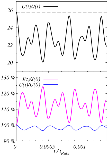
Figure 1: (color online). Bose-Hubbard model with time-dependent Wannier functions (TDBH model). Shown is the time-dependence of the hopping and the interaction parameters $J(t)$ and $U(t)$ for a quench. Initially a system of $N=20$ bosons is prepared in the noninteracting ground state of a two-site ring lattice, see text for details. At $t=0$ the interaction strength is switched on to $U(0)/J(0)=25.8$ and the resulting dynamics is monitored. Top: $U(t)/J(t)$ oscillates rapidly with a large amplitude between about $25.8$ and $20$. Note the time-scale. $U(t)/J(t)$ is always smaller than its initial value which is the value of the BH model (dashed line). Bottom: $J(t)$ and $U(t)$ oscillate in time. $J(t)$ is always larger, $U(t)$ always smaller than its initial value. The oscillations are due to multi-band excitations induced by the quench. $J(t)$ varies over almost $25\%$, $U(t)$ over about $4\%$ of its initial value. The hopping process is obviously much more involved than what the time-independent parameter $J$ of the BH model can capture. The respective BH results are constant in time and equal to the values at $t=0$. All quantities shown are dimensionless.

On physical grounds it can be anticipated that the sudden increase of the (repulsive) interaction strength will lead to breathing oscillations of the one-particle density $\rho^{(1)}(x|x;t)$ in each of the wells. However, as the final interaction strength is not very strong these density oscillations should have a small amplitude only. It is important to note that for the BH model the ratio of the interaction and the hopping parameter $U/J$ is the only relevant parameter and also that it is constant in time after the quench. In the TDBH model on the other hand we expect $U(t)/J(t)$ to vary, because the Wannier functions can change in time. This is indeed the case. Fig. 1 shows the parameters $U(t)$ and $J(t)$ of the TDBH model and their ratio $U(t)/J(t)$ as a function of time. As expected, right after the quench the density in each well expands and hence $U(t)$ decreases, while $J(t)$ increases. Both parameters then oscillate at a high frequency. Note the short time-scale. The interaction broadens the density and therefore $U(t)$ ($J(t)$) is always smaller (larger) than its value at time $t=0$. As $J(t)$ depends on the overlap of adjacent time-dependent Wannier functions, it is very sensitive to any variation of their tails. It varies over almost $25\%$! The interaction parameter $U(t)$ is sensitive to variations of the bulk density and varies only over about $4\%$. As a result, the ratio $U(t)/J(t)$ of the TDBH model varies between $25.8$ and $20$, a range of about $25\%$. In contrast, for the BH model the ratio $U/J=25.8$ is constant at all times as mentioned above. The rapid oscillations of $U(t)$ and $J(t)$ are only possible because the Wannier functions can evolve in the space of multiple bands and thus represent multi-band excitations. This clearly demonstrates the advantages of the TDBH model over the BH model in reproducing the physics of the quench studied here.

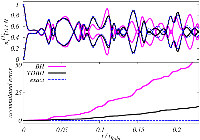
Figure 2: (color online). Quench dynamics in a double well as in Fig. 1. Top: shown are the natural occupations of the BH (solid magenta lines) model, the TDBH (solid black lines) model and the exact (dashed blue lines) result as a function of time. Starting from a fully condensed state the dynamics is intricate and shows oscillations between partially condensed and fragmented states. The TDBH result follows the exact one closely and in particular reproduces the frequencies of the oscillations well. The BH result deviates quickly from the exact one. Bottom: the accumulated error (see text) of the TDBH model is always smaller than that of the BH model and grows much more slowly. All quantities shown are dimensionless.

We now turn to the question about the nature of the quantum state after the quench and to longer time-scales. We first focus on the eigenvalues of the first-order reduced density matrix, the natural occupation numbers $n_{i}^{(1)}(t)$, which determine the degree to which the system is condensed or fragmented PeO56 ; NoS82 . In Fig. 2 (top) the natural occupation numbers of the TDBH model are shown together with those of the BH model. For comparison also the numerically exact dynamics of the time-dependent many-body Schrödinger equation is shown, obtained using the multiconfigurational time-dependent Hartree for bosons method. For details see the literature MCTDHB1 ; MCTDHB2 . Note that the time-scale is now more than a hundred times larger compared to Fig. 1. It is clearly seen that all three results display oscillations between fragmented and partially condensed states. For the first few oscillations the three results essentially coincide, which implies that for this problem the natural occupation numbers are not very sensitive to the previously discussed multi-band excitations. However, after a few oscillations between condensed and fragmented states the BH result deviates substantially from the exact one. On the other hand, the TDBH result follows the exact one closely for many oscillations. In Fig. 2 (bottom) the accumulated error of the BH model, defined as the accumulated difference $\frac{1}{N}\int_{0}^{t}dt^{\prime}|n_{1,BH}^{(1)}(t^{\prime})-n_{1,exact}^{(1)}(t^{\prime})|$ between the largest natural occupation number of the BH model and the numerically exact result are shown, together with the analogous quantity of the TDBH model. The accumulated error of the TDBH model is always smaller than that of the BH model and grows more slowly, which means that also on longer time-scales the TDBH model captures the true physics much better than the BH model.

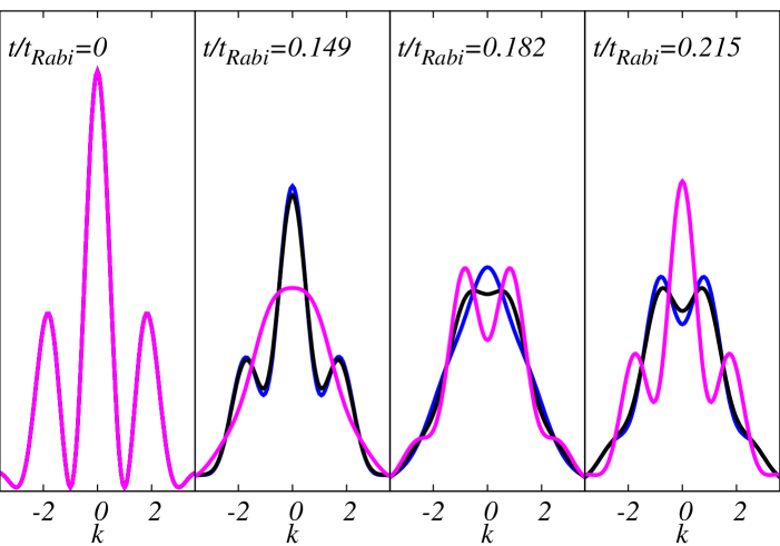
Figure 3: (color online). Quench dynamics in a double well as in Fig. 1. Shown is the one-particle momentum distribution of the BH (solid magenta lines) model, the TDBH (solid black lines) and the exact result (solid blue lines) at different times. The initial state is fully coherent and for a short time the three results have similar momentum distributions (not shown). The TDBH result is always much closer to the exact one than the BH result. Differences of the TDBH (BH) result relative to the exact one always occur when the natural occupations differ, see Fig. 2. All quantities shown are dimensionless.

We will now discuss the implications of the differences of the natural occupation numbers on observables. The rapid density oscillations discussed earlier have a very small amplitude, and consequently hardly any dynamics is visible in real space. However, a substantial dynamics occurs in momentum space. Fig. 3 shows the one-particle momentum distribution $\rho^{(1)}(k|k;t)$ of the exact, the TDBH and the BH result at $t=0$ where they all coincide, and at later times where differences have developed. The momentum distribution of the TDBH model is always closer to the exact one and follows it for a long time, whereas that of the BH model deviates quickly. Here, the TDBH model allows to obtain the precise multi-band nonequilibrium dynamics essentially at the cost of a single-band model. Of course, in order to obtain the exact result the terms that were neglected so far in Eq. (2) have to be included into the model, e.g., the terms responsible for correlated tunneling. Thus, the advantages of the TDBH model over the BH model have been clearly proven.

In this work we have generalized the concept of lattice models by letting their Wannier functions become time-dependent. For such lattice models equations of motion can be derived from the variational principle, leading to variationally optimal lattice models that can efficiently incorporate multi-band physics. The concept is applicable to both nonequilibrium dynamics as well as statics. In the latter case the ground state can be computed using imaginary time-propagation. The variational principle ensures that for identical initial conditions the optimal lattice model improves on the original lattice model, if the latter contains the terms of the full many-body Hamiltonian relevant to the problem at hand. Since the numerical effort of the optimal and standard lattice models are comparable, the former can also be used to assess the quality of the latter: if the respective results differ noticeably, the standard lattice model is inapplicable. As an application, we have presented the equations of motion for the TDBH model, i.e., the Bose-Hubbard model with time-dependent Wannier functions. We then studied a quantum quench problem in a double-well using the TDBH model. Multi-band excitations were found that resulted in high-frequency, large amplitude oscillations of the hopping and interaction parameters. Such phenomena are not accessible to the BH model. On a longer time-scale the multi-band excitations also affect the nature of the quantum state and the momentum distribution. We have compared the results of the TDBH and the BH model for the natural occupation numbers and the momentum distributions with numerically exact ones of the many-body Schrödinger equation. For this problem, we find that the TDBH results follow the exact ones for a long time, while the BH results deviate quickly. Interestingly, the numerical effort for solving the equations of motion of the TDBH model is essentially the same as for the BH model, see the appendix for details.

Summarizing, standard lattice models can be greatly extended at little extra cost through the use of time-dependent Wannier functions. It will be interesting to examine what other physical multi-band phenomena are accessible to such time-dependent lattice models, e.g., in disordered media or in the case of the fermionic Hubbard model. As a further direction we suggest to combine 1D optimal lattice models with the recently developed adaptive time-dependent density-matrix renormalization group methods t1 ; t2 ; t3 to treat non-equilibrium dynamics of larger lattice systems, as is presently done utilizing standard lattice models.

*

Appendix A Derivation and discussion of the equations of motion of the TDBH model

We will now derive Eqs. (Optimal time-dependent lattice models for nonequilibrium dynamics) and discuss their properties. Using the ansatz for the many-body wave function $|\Psi(t)\rangle=\sum_{\vec{n}}C_{\vec{n}}(t)\left|\vec{n};t\right>$ given above, the action functional of the TDBH model reads

$$S\left[\{C_{\vec{n}}\},\{d_{k}^{\alpha}\}\right]=\int dt\biggl{\{}\left<\Psi\left|\hat{H}_{TDBH}-i\frac{\partial}{\partial t}\right|\Psi\right>-\sum_{i}\mu_{i}(t)\left[\left<w_{i}(t)|w_{i}(t)\right>-1\right]\biggr{\}},$$ (4)

where the Lagrange multipliers are introduced to ensure orthonormality between the time-dependent Wannier functions. Note that Eq. (1) implies that time-dependent Wannier functions on different lattice sites are orthogonal by construction. In order to take functional derivatives it is useful to express the expectation value $\langle\Psi|\hat{H}_{TDBH}-i\frac{\partial}{\partial t}|\Psi\rangle$ as an explicit function of the amplitudes $\{d_{k}^{\alpha}(t)\}$ and expansion coefficients $\{C_{\vec{n}}(t)\}$. On the one hand $\langle\Psi|\hat{H}_{TDBH}-i\frac{\partial}{\partial t}|\Psi\rangle$ can be written as:

$$\biggl{<}\Psi\biggl{|}\hat{H}_{TDBH}-i\frac{\partial}{\partial t}\biggr{|}\Psi\biggr{>}=\sum_{\vec{n}}C^{\ast}_{\vec{n}}(t)\biggl{[}\sum_{\vec{n}^{\prime}}\biggl{<}\vec{n};t\biggl{|}\hat{H}_{TDBH}-i\frac{\partial}{\partial t}\biggr{|}\vec{n}^{\prime};t\biggr{>}C_{\vec{n^{\prime}}}(t)-i\frac{\partial C_{\vec{n}}(t)}{\partial t}\biggr{]}.$$ (5)

Using Eq. (5) we now require stationarity of the action functional with respect to variations of the coefficients, $0=\frac{\delta S}{\delta C^{\ast}_{\vec{n}}(t)}$, and obtain:

$$\sum_{\vec{n}^{\prime}}\left<\vec{n};t\left|\hat{H}_{TDBH}-i\frac{\partial}{\partial t}\right|\vec{n}^{\prime};t\right>C_{\vec{n^{\prime}}}(t)=i\frac{\partial C_{\vec{n}}(t)}{\partial t}.$$ (6)

On the other hand $\langle\Psi|\hat{H}_{TDBH}-i\frac{\partial}{\partial t}|\Psi\rangle$ can also be written as:

$$\left<\Psi\left|\hat{H}_{TDBH}-i\frac{\partial}{\partial t}\right|\Psi\right>=\sum_{k,q=k,k\pm 1}\sum_{\alpha,\beta}^{\nu}\rho_{kq}(t)\,{d_{k}^{\alpha}}^{\ast}(t)\left(h_{k_{\alpha}q_{\beta}}-i\delta_{kq}\delta_{\alpha\beta}\frac{\partial}{\partial t}\right)d_{q}^{\beta}(t)$$

$$+\frac{1}{2}\sum_{k}\sum_{\alpha\beta\gamma\delta}\rho_{kkkk}(t)\,{d_{k}^{\alpha}}^{\ast}(t){d_{k}^{\beta}}^{\ast}(t)\,U_{k^{\alpha}k^{\beta}k^{\gamma}k^{\delta}}\,d_{k}^{\gamma}(t)d_{k}^{\delta}(t)-i\sum_{\vec{n}}C_{\vec{n}}(t)\frac{\partial C_{\vec{n}}^{\ast}(t)}{\partial t},$$ (7)

where $h_{k^{\alpha}q^{\beta}}=\langle w_{k}^{\alpha}|\hat{h}|w_{q}^{\beta}\rangle$, $U_{k^{\alpha}k^{\beta}k^{\gamma}k^{\delta}}=\lambda_{0}\int dx{w_{k}^{\alpha}}(x)^{\ast}{w_{k}^{\beta}}(x)^{\ast}w_{k}^{\delta}(x)w_{k}^{\delta}(x)$ and we have used $\langle w_{k}^{\alpha}|w_{q}^{\beta}\rangle=\delta_{kq}\delta_{\alpha\beta}$. Note that the matrix elements of the first- and second-order reduced density matrices are functions of the coefficients $\{C_{\vec{n}}(t)\}$ only. Using Eq. (A) we now require stationarity of the action functional with respect to variations of the time-dependent amplitudes, $0=\frac{\delta S}{\delta{d^{\alpha}_{k}}^{\ast}(t)}$, and obtain

$$\sum_{q=k,k\pm 1}\rho_{kq}(t)\langle w_{k}^{\alpha}|\hat{h}|w_{q}(t)\rangle+\rho_{kkkk}(t)\langle w_{k}^{\alpha}|\hat{U}_{kk}(t)|w_{k}(t)\rangle=\mu_{k}(t)\langle w_{k}^{\alpha}|w_{k}(t)\rangle+i\rho_{kk}(t)\langle w_{k}^{\alpha}|\dot{w}_{k}(t)\rangle,$$ (8)

for $\alpha=1,\dots,\nu$ and $k=1,\dots,M$, where we have used $d_{k}^{\alpha}(t)=\langle w_{k}^{\alpha}|w_{k}(t)\rangle$. The Lagrange multipliers $\mu_{k}(t)$ can be determined from Eqs. (8), which upon resubstituting the result, multiplying each equation by $|w_{k}^{\alpha}\rangle$ and summing over $\alpha$ gives

$$i\rho_{kk}(t)\hat{P}_{k}(t)|\dot{w}_{k}(t)\rangle = \hat{P}_{k}(t)\left[\sum_{q=k,k\pm 1}\rho_{kq}(t)\hat{h}|w_{q}(t)\rangle+\rho_{kkkk}(t)\hat{U}_{kk}(t)|w_{k}(t)\rangle\right].$$ (9)

By including the additional phase factor $e^{-\int^{t}dt^{\prime}\langle w_{k}(t)|\dot{w}_{k}(t)\rangle}$ into the definition of $|w_{k}(t)\rangle$, we find that $\langle w_{k}(t)|\dot{w}_{k}(t)\rangle=0$, and that Eqs. (9) and (6) reduce to Eqs. (Optimal time-dependent lattice models for nonequilibrium dynamics).

Let us briefly discuss the numerical advantage of using time-dependent Wannier functions over conventional ones. The fundamental difficulty in solving quantum lattice models lies in the fact that the dimension of the many-particle Hilbert space grows very quickly as a function of the number of particles $N$ and the number of lattice sites $M$. In the case of the BH model the length of the vector ${\bf C}$ is $\binom{N+M-1}{N}$. This is also the length of the vector ${\bf C}$ in the TDBH model since we have only replaced conventional Wannier functions by time-dependent ones. However, since each of the time-dependent Wannier functions can take on any shape allowed by Eq. (1), a much larger Hilbert space is available to the variational principle. Note that the number of bands $\nu$ in which each time-dependent Wannier function is expanded does not enter the above dimension formula. If $\nu$ is restricted to one, the time-dependent Wannier functions become time-independent and only the second of Eqs. (Optimal time-dependent lattice models for nonequilibrium dynamics) needs to be solved. In this case Eqs. (Optimal time-dependent lattice models for nonequilibrium dynamics) reduce to the equations of motion of the BH model. If $\nu>1$ the coupled system, Eqs. (Optimal time-dependent lattice models for nonequilibrium dynamics), needs to be solved. Then, the additional numerical cost consists of propagating not only the coefficients $\{C_{\vec{n}}(t)\}$, but also the time-dependent Wannier functions $\{w_{k}(x,t)\}$, i.e., $M$ additional nonlinear equations have to be solved. For all but the smallest numbers of particles and lattice sites, this extra effort is much smaller than the effort needed to propagate the second of Eqs. (Optimal time-dependent lattice models for nonequilibrium dynamics). Note that the alternative of enlarging the Hilbert space by using multiple, say $\kappa>1$, bands of conventional (static) Wannier functions, would increase the length of the vector ${\bf C}$ to $\binom{N+\kappa M-1}{N}$. This illustrates why it is crucial to use time-dependent Wannier functions: time-dependent Wannier functions allow to keep the numerical effort of a time-dependent lattice model very close to that of the respective standard lattice model while efficiently incorporating multi-band physics. Since all parameters, i.e., the coefficients $\{C_{\vec{n}}(t)\}$ and the Wannier functions $\{w_{k}(x,t)\}$ are at all times determined by the variational principle, the lattice model is optimal.

- (1) S. Sachdev, Quantum Phase Transitions (Cambridge University Press, 1999).
- (2) G. H. Wannier, Phys. Rev. 52, 191 (1937).
- (3) W. Jones and N. H. March, Theoretical Solid State Physics Volume 1: Perfect Lattices in Equilibrium (Dover, 1985).
- (4) M. P. A. Fisher et al., Phys. Rev. B 40, 546 (1989).
- (5) J. Hubbard, Proc. R. Soc. Lond. A 276, 238 (1963).
- (6) O. E. Alon et al., Phys. Rev. Lett. 95, 030405 (2005).
- (7) V. W. Scarola and S. Das Sarma, Phys. Rev. Lett. 95, 033003 (2005).
- (8) A. Isacsson and S. M. Girvin, Phys. Rev. A 72, 053604 (2005).
- (9) J. Li et al., New J. Phys. 8 154, (2006).
- (10) V. M. Stojanović et al., Phys. Rev. Lett. 101, 125301 (2008).
- (11) D.-S. Lühmann et al., Phys. Rev. Lett. 101, 050402 (2008).
- (12) T. Best et al., Phys. Rev. Lett. 102, 030408 (2009).
- (13) J. Larson et al., Phys. Rev. A 79, 033603 (2009).
- (14) K. Sakmann et al., Phys. Rev. Lett. 103, 220601 (2009); Sakmann K, et al., Phys. Rev. A 82 013620 (2010).
- (15) S. Will et al., Nature 465, 197 (2010).
- (16) P. Kramer and M. Saraceno, Geometry of the Time-Dependent Variational Principle in Quantum Mechanics (Springer, Berlin, 1981) Lecture Notes in Physics vol 140.
- (17) O. E. Alon et al., Phys. Rev. A 77, 033613 (2008).
- (18) C. Lee, Phys. Rev. Lett. 97, 150402 (2006).
- (19) D. R. Dounas-Frazer et al., Phys. Rev. Lett. 99, 200402 (2007).
- (20) Y. Khodorkovsky et al., Phys. Rev. Lett. 100, 220403 (2008).
- (21) P. Cheinet et al., Phys. Rev. Lett. 101, 090404 (2008).
- (22) E. M. Graefe et al., Phys. Rev. Lett. 101, 150408 (2008).
- (23) D. Witthaut et al., Phys. Rev. Lett. 101, 200402 (2008).
- (24) E. Boukobza et al., Phys. Rev. Lett. 102, 180403 (2009).
- (25) K. Smith-Mannschott et al., Phys. Rev. Lett. 102, 230401 (2009).
- (26) J. Wang and J. Gong, Phys. Rev. Lett. 102, 244102 (2009).
- (27) J. Gong et al., Phys. Rev. Lett. 103, 133002 (2009).
- (28) E. Boukobza et al., Phys. Rev. Lett. 104, 240402 (2010).
- (29) C. Kollath et al., Phys. Rev. Lett. 98, 180601 (2007).
- (30) I. Klich et al., Phys. Rev. Lett. 99, 205303 (2007).
- (31) M. Rigol et al., Nature 452, 854 (2008).
- (32) G. Roux, Phys. Rev. A 81, 053604 (2010).
- (33) O. Penrose and L. Onsager, Phys. Rev. 104, 576 (1956).
- (34) P. Nozières, D. Saint James, J. Phys. France 43, 1133 (1982); P. Nozières, in Bose-Einstein Condensation, edited by A. Griffin, D. W. Snoke, and S. Stringari (Cambridge University Press, 1996) ISBN 9780521589901.
- (35) A. I. Streltsov et al., Phys. Rev. Lett. 99, 030402 (2007).
- (36) G. Vidal, Phys. Rev. Lett. 93, 040502 (2004).
- (37) A. Daley et al., J. Stat. Mech.: Theory Exp. P04005 (2004).
- (38) S. R. White and A. E. Feiguin, Phys. Rev. Lett. 93, 076401 (2004).