On two approaches to 3-dimensional TQFTs

Abstract.

We prove that $|M|_{\mathcal{C}}=\tau_{\mathcal{Z}(\mathcal{C})}(M)$ for any closed oriented 3-manifold $M$ and for any spherical fusion category $\mathcal{C}$ of non-zero dimension. Here $|M|_{\mathcal{C}}$ is the Turaev-Viro-Barrett-Westbury state sum invariant of $M$ derived from  $\mathcal{C}$, $\mathcal{Z}(\mathcal{C})$ is the Drinfeld-Joyal-Street center of $\mathcal{C}$, and $\tau_{\mathcal{Z}(\mathcal{C})}(M)$ is the Reshetikhin-Turaev surgery invariant of $M$ derived from $\mathcal{Z}(\mathcal{C})$.

Introduction

Two fundamental constructions of 3-dimensional topological quantum field theories (TQFTs) are due to Reshetikhin-Turaev [RT] and Turaev-Viro [TV]. The RT-construction is widely viewed as a mathematical realization of Witten’s Chern-Simons TQFT, see [Wi]. The TV-construction is closely related to the Ponzano-Regge state-sum model for 3-dimensional quantum gravity, see [Ca]. The first connections between these two constructions were established by Walker [Wa] and Turaev [Tu]. In 1995, the first named author conjectured a more general connection between these constructions. This connection may be formulated as the identity $|M|_{\mathcal{C}}=\tau_{\mathcal{Z}(\mathcal{C})}(M)$, see below for a detailed statement. The aim of our paper is to prove this conjecture.

The Turaev-Viro approach derives TQFTs from spherical fusion categories. We define a fusion category as a monoidal category with compatible left and right dualities such that all objects are direct sums of simple objects and the number of isomorphism classes of simple objects is finite. The condition of sphericity says that the left and right dimensions of all objects are equal. A spherical fusion category has a numerical dimension, which we suppose to be non-zero throughout the introduction. The original TV-construction [TV] applies to categories of representations of the quantum group $U_{q}(sl_{2}(\mathbb{C}))$ at roots of unity. This was extended to modular categories (i.e., to spherical fusion categories with braiding) in [Tu]. At about the same time, A. Ocneanu observed that the use of the braiding may be avoided. This was formalized by Barrett and Westbury [BW1] (see also [GK]) who derived a topological invariant $|M|_{\mathcal{C}}$ of an arbitrary closed oriented 3-manifold $M$ from a spherical fusion category $\mathcal{C}$. The definition of $|M|_{\mathcal{C}}$ goes by considering a certain state sum on a triangulation of $M$ and proving that this sum depends only on $M$ and not on the choice of triangulation. The key algebraic ingredients of the state sum are the so-called $6j$-symbols associated with $\mathcal{C}$.

The Reshetikhin-Turaev construction of 3-manifold invariants uses as the main algebraic ingredient a modular category $\mathcal{B}$. This construction associates with every closed oriented 3-manifold $M$ a numerical invariant $\tau_{\mathcal{B}}(M)$. Its definition is based on surgery presentations of $M$ by links in the 3-sphere.

For every monoidal category $\mathcal{C}$, Joyal and Street [JS] and Drinfeld (unpublished, see Majid [Maj]) defined a braided monoidal category $\mathcal{Z}(\mathcal{C})$ called the center of $\mathcal{C}$. A fundamental theorem of Müger [Mü2] says that the center of a spherical fusion category $\mathcal{C}$ over an algebraically closed field is modular. Combining with the results mentioned above, we observe that such a $\mathcal{C}$ gives rise to two 3-manifold invariants: $|M|_{\mathcal{C}}$ and $\tau_{\mathcal{Z}(\mathcal{C})}(M)$. We prove in the present paper that these invariants are equal, i.e., for all $M$,

(1) $$|M|_{\mathcal{C}}=\tau_{\mathcal{Z}(\mathcal{C})}(M).$$

This was previously known in several special cases: when $\mathcal{C}$ is modular [Tu, Wa], when $\mathcal{C}$ is the category of bimodules associated with a subfactor [KSW], and when $\mathcal{C}$ is the category of representations of a finite group. For modular $\mathcal{C}$, the category $\mathcal{Z}(\mathcal{C})$ is braided equivalent to the Deligne tensor product $\mathcal{C}\boxtimes\overline{\mathcal{C}}$, where $\overline{\mathcal{C}}$ is the mirror of $\mathcal{C}$, and therefore Formula (1) can be rewritten as

$$|M|_{\mathcal{C}}=\tau_{\mathcal{C}\boxtimes\overline{\mathcal{C}}}(M)=\tau_{\mathcal{C}}(M)\,\tau_{\overline{\mathcal{C}}}(M)=\tau_{\mathcal{C}}(M)\,\tau_{\mathcal{C}}(-M),$$

where $-M$ is $M$ with opposite orientation. If $\mathcal{C}$ is a unitary modular category, then $\tau_{\mathcal{C}}(-M)=\overline{\tau_{\mathcal{C}}(M)}$ and so $|M|_{\mathcal{C}}=|\tau_{\mathcal{C}}(M)|^{2}$.

Formula (1) relates two categorical approaches to 3-manifold invariants through the categorical center. This relationship sheds new light on both approaches and shows, in particular, that the RT-construction is more general than the state sum construction. For further corollaries of Formula (1), see Section 11.

The proof of Formula (1) is based on topological quantum field theory (TQFT). For a modular category $\mathcal{B}$, the invariants $\tau_{\mathcal{B}}(M)$ extend to a 3-dimensional TQFT $\tau_{\mathcal{B}}$ derived from $\mathcal{B}$, see [RT]. The invariant $|M|_{\mathcal{C}}$ also extends to a 3-dimensional state sum TQFT $|.|_{\mathcal{C}}$ which we define here in terms of state sums on skeletons of 3-manifolds. It is crucial for the proof of Formula (1) that we allow non-generic skeletons, i.e., skeletons with edges incident to $\geq 4$ regions. In particular, we give two different state sums on any triangulation $t$ of a closed oriented 3-manifold $M$: the one in [TV, BW1] and a new one. In the former, the labels are attributed to the edges and the Boltzmann weights are the $6j$-symbols computed in the tetrahedra; in the latter, the labels are attributed to the faces and the Boltzmann weights are computed in the vertices. The existence of two different state sums is due to the fact that the triangulation $t$ gives rise to two different skeletons of $M$: the 2-skeleton of the cellular decomposition of $M$ dual to $t$ and the 2-skeleton of $t$ itself. (It is non-obvious but true that these two state sums are equal.)

Our main theorem claims that for any spherical fusion category $\mathcal{C}$ over an algebraically closed field, the TQFTs $|.|_{\mathcal{C}}$ and $\tau_{\mathcal{Z}(\mathcal{C})}$ are isomorphic:

$$|\Sigma|_{\mathcal{C}}\simeq\tau_{\mathcal{Z}(\mathcal{C})}(\Sigma)\quad\text{and}\quad|M|_{\mathcal{C}}\simeq\tau_{\mathcal{Z}(\mathcal{C})}(M)$$

for any oriented closed surface $\Sigma$ and any oriented 3-cobordism $M$. The proof involves a detailed study of transformations of skeletons of 3-manifolds and the computation of the coend of $\mathcal{Z}(\mathcal{C})$ provided by the theory of Hopf monads in monoidal categories due to Bruguières and Virelizier [BV2]. Another important ingredient of the proof is an extension of $|M|_{\mathcal{C}}$ to a state sum invariant $|M,L|_{\mathcal{C}}$ of a $\mathcal{Z}(\mathcal{C})$-colored framed link $L$ in a 3-manifold $M$.

After the appearance of the present paper on arXiv, Balsam and Kirillov [Ba1, Ba2, BK] found a different proof of (1) based on the concept of an extended TQFT.

The paper is organized as follows. Sections 1–4 deal with preliminaries on monoidal and fusion categories and the associated invariants of colored graphs. In Sections 5–9 we construct the TQFT $|.|_{\mathcal{C}}$. In Sections 10 and 11 we recall the necessary definitions from the theory of modular categories and state our main theorems. A proof of these theorems is given in Sections 12–15. Though we do not specifically use $6j$-symbols, we include for completeness an appendix summarizing their properties.

The authors are indebted to N. Ivanov and S. Matveev for helpful discussions. The work of V. Turaev on this paper was partially supported by the NSF grant DMS-0904262. A. Virelizier was partially supported by the ANR grant GESAQ.

Throughout the paper, the symbol $\Bbbk$ denotes a commutative ring.

1. Pivotal and spherical categories

We review several classes of monoidal categories needed in the sequel.

1.1. Pivotal categories ([Mal])

By a pivotal (or sovereign) category, we mean a strict monoidal category $\mathcal{C}$ with unit object $\mathbb{1}$ such that to each object $X\in\mathrm{Ob}(\mathcal{C})$ there are associated a dual object $X^{*}\in\mathrm{Ob}(\mathcal{C})$ and four morphisms

$$\mathrm{ev}_{X}\colon X^{*}\otimes X\to\mathbb{1},\qquad\mathrm{coev}_{X}\colon\mathbb{1}\to X\otimes X^{*},$$

$$\widetilde{\mathrm{ev}}_{X}\colon X\otimes X^{*}\to\mathbb{1},\qquad\widetilde{\mathrm{coev}}_{X}\colon\mathbb{1}\to X^{*}\otimes X,$$

satisfying the following conditions:

1. For every $X\in\mathrm{Ob}(\mathcal{C})$, the pair $(\mathrm{ev}_{X},\mathrm{coev}_{X})$ is a left duality for $X$, i.e.,

   $$(\mathrm{id}_{X}\otimes\mathrm{ev}_{X})(\mathrm{coev}_{X}\otimes\mathrm{id}_{X})=\mathrm{id}_{X}\quad{\rm{and}}\quad(\mathrm{ev}_{X}\otimes\mathrm{id}_{X^{*}})(\mathrm{id}_{X^{*}}\otimes\mathrm{coev}_{X})=\mathrm{id}_{X^{*}};$$

2. For every $X\in\mathrm{Ob}(\mathcal{C})$, the pair $(\widetilde{\mathrm{ev}}_{X},\widetilde{\mathrm{coev}}_{X})$ is a right duality for $X$, i.e.,

   $$(\widetilde{\mathrm{ev}}_{X}\otimes\mathrm{id}_{X})(\mathrm{id}_{X}\otimes\widetilde{\mathrm{coev}}_{X})=\mathrm{id}_{X}\quad{\rm{and}}\quad(\mathrm{id}_{X^{*}}\otimes\widetilde{\mathrm{ev}}_{X})(\widetilde{\mathrm{coev}}_{X}\otimes\mathrm{id}_{X^{*}})=\mathrm{id}_{X^{*}};$$

3. For every morphism $f\colon X\to Y$ in $\mathcal{C}$, the left dual

   $$f^{*}=(\mathrm{ev}_{Y}\otimes\mathrm{id}_{X^{*}})(\mathrm{id}_{Y^{*}}\otimes f\otimes\mathrm{id}_{X^{*}})(\mathrm{id}_{Y^{*}}\otimes\mathrm{coev}_{X})\colon Y^{*}\to X^{*}$$

   is equal to the right dual

   $$f^{*}=(\mathrm{id}_{X^{*}}\otimes\widetilde{\mathrm{ev}}_{Y})(\mathrm{id}_{X^{*}}\otimes f\otimes\mathrm{id}_{Y^{*}})(\widetilde{\mathrm{coev}}_{X}\otimes\mathrm{id}_{Y^{*}})\colon Y^{*}\to X^{*};$$

4. For all $X,Y\in\mathrm{Ob}(\mathcal{C})$, the morphisms $X^{*}\otimes Y^{*}\to(Y\otimes X)^{*}$ defined as

   $$(\mathrm{ev}_{X}\otimes\mathrm{id}_{(Y\otimes X)^{*}})(\mathrm{id}_{X^{*}}\otimes\mathrm{ev}_{Y}\otimes\mathrm{id}_{X\otimes(Y\otimes X)^{*}})(\mathrm{id}_{X^{*}\otimes Y^{*}}\otimes\mathrm{coev}_{Y\otimes X})$$

   and as

   $$(\mathrm{id}_{(Y\otimes X)^{*}}\otimes\widetilde{\mathrm{ev}}_{Y})(\mathrm{id}_{(Y\otimes X)^{*}\otimes Y}\otimes\widetilde{\mathrm{ev}}_{X}\otimes\mathrm{id}_{Y^{*}})(\widetilde{\mathrm{coev}}_{Y\otimes X}\otimes\mathrm{id}_{X^{*}\otimes Y^{*}})$$

   are equal (these morphisms are called monoidal constraints);

5. $\mathrm{ev}_{\mathbb{1}}=\widetilde{\mathrm{ev}}_{\mathbb{1}}\colon\mathbb{1}^{*}\to\mathbb{1}$ (or, equivalently, $\mathrm{coev}_{\mathbb{1}}=\widetilde{\mathrm{coev}}_{\mathbb{1}}\colon\mathbb{1}\to\mathbb{1}^{*}$).

Note that the morphisms $\mathrm{ev}_{\mathbb{1}}$ and $\mathrm{coev}_{\mathbb{1}}$ (respectively, $\widetilde{\mathrm{ev}}_{\mathbb{1}}$ and $\widetilde{\mathrm{coev}}_{\mathbb{1}}$) are mutually inverse isomorphisms. The monoidal constraints in (d) also are isomorphisms. By abuse of notation, we will suppress these isomorphisms in the formulas. For example, we will write $(f\otimes g)^{*}=g^{*}\otimes f^{*}$ for morphisms $f,g$ in $\mathcal{C}$.

1.2. Traces and dimensions

For an endomorphism $f$ of an object $X$ of a pivotal category $\mathcal{C}$, one defines the left and right traces $\mathrm{tr}_{l}(f),\mathrm{tr}_{r}(f)\in\mathrm{End}_{\mathcal{C}}(\mathbb{1})$ by

$$\mathrm{tr}_{l}(f)=\mathrm{ev}_{X}(\mathrm{id}_{X^{*}}\otimes f)\widetilde{\mathrm{coev}}_{X}\quad{\text{and}}\quad\mathrm{tr}_{r}(f)=\widetilde{\mathrm{ev}}_{X}(f\otimes\mathrm{id}_{X^{*}})\mathrm{coev}_{X}.$$

Both traces are symmetric: $\mathrm{tr}_{l}(gh)=\mathrm{tr}_{l}(hg)$ and $\mathrm{tr}_{r}(gh)=\mathrm{tr}_{r}(hg)$ for any morphisms $g\colon X\to Y$ and $h\colon Y\to X$ in $\mathcal{C}$. Also $\mathrm{tr}_{l}(f)=\mathrm{tr}_{r}(f^{*})=\mathrm{tr}_{l}(f^{**})$ for any endomorphism $f$ of an object (and similarly with $l,r$ exchanged). If

(2) $$\alpha\otimes\mathrm{id}_{X}=\mathrm{id}_{X}\otimes\alpha\quad\text{for all $\alpha\in\mathrm{End}_{\mathcal{C}}(\mathbb{1})$ and $X\in\mathrm{Ob}(\mathcal{C})$,}$$

then $\mathrm{tr}_{l},\mathrm{tr}_{r}$ are $\otimes$-multiplicative: $\mathrm{tr}_{l}(f\otimes g)=\mathrm{tr}_{l}(f)\,\mathrm{tr}_{l}(g)$ and $\mathrm{tr}_{r}(f\otimes g)=\mathrm{tr}_{r}(f)\,\mathrm{tr}_{r}(g)$ for all endomorphisms $f,g$ of objects of $\mathcal{C}$.

The left and right dimensions of $X\in\mathrm{Ob}(\mathcal{C})$ are defined by $\dim_{l}(X)=\mathrm{tr}_{l}(\mathrm{id}_{X})$ and $\dim_{r}(X)=\mathrm{tr}_{r}(\mathrm{id}_{X})$. Clearly, $\dim_{l}(X)=\dim_{r}(X^{*})=\dim_{l}(X^{**})$ (and similarly with $l,r$ exchanged). Note that isomorphic objects have the same dimensions and $\dim_{l}(\mathbb{1})=\dim_{r}(\mathbb{1})=\mathrm{id}_{\mathbb{1}}$. If $\mathcal{C}$ satisfies (2), then left and right dimensions are $\otimes$-multiplicative: $\dim_{l}(X\otimes Y)=\dim_{l}(X)\dim_{l}(Y)$ and $\dim_{r}(X\otimes Y)=\dim_{r}(X)\dim_{r}(Y)$ for any $X,Y\in\mathrm{Ob}(\mathcal{C})$.

1.3. Penrose graphical calculus

We represent morphisms in a category $\mathcal{C}$ by plane diagrams to be read from the bottom to the top. The diagrams are made of oriented arcs colored by objects of $\mathcal{C}$ and of boxes colored by morphisms of $\mathcal{C}$. The arcs connect the boxes and have no mutual intersections or self-intersections. The identity $\mathrm{id}_{X}$ of $X\in\mathrm{Ob}(\mathcal{C})$, a morphism $f\colon X\to Y$, and the composition of two morphisms $f\colon X\to Y$ and $g\colon Y\to Z$ are represented as follows:

$\mathrm{id}_{X}=$ \psfrag{X}[Bc][Bc]{\scalebox{0.7}{$X$}}\psfrag{Y}[Bc][Bc]{\scalebox{0.7}{$Y$}}\psfrag{h}[Bc][Bc]{\scalebox{0.8}{$f$}}\psfrag{g}[Bc][Bc]{\scalebox{0.8}{$g$}}\psfrag{Z}[Bc][Bc]{\scalebox{0.7}{$Z$}}\includegraphics{identitymorph.eps}  , $f=$ \psfrag{X}[Bc][Bc]{\scalebox{0.7}{$X$}}\psfrag{Y}[Bc][Bc]{\scalebox{0.7}{$Y$}}\psfrag{h}[Bc][Bc]{\scalebox{0.8}{$f$}}\psfrag{g}[Bc][Bc]{\scalebox{0.8}{$g$}}\psfrag{Z}[Bc][Bc]{\scalebox{0.7}{$Z$}}\includegraphics{morphism.eps} , and  $gf=$ \psfrag{X}[Bc][Bc]{\scalebox{0.7}{$X$}}\psfrag{Y}[Bc][Bc]{\scalebox{0.7}{$Y$}}\psfrag{h}[Bc][Bc]{\scalebox{0.8}{$f$}}\psfrag{g}[Bc][Bc]{\scalebox{0.8}{$g$}}\psfrag{Z}[Bc][Bc]{\scalebox{0.7}{$Z$}}\includegraphics{morphismcompo.eps}  .

If $\mathcal{C}$ is monoidal, then the monoidal product of two morphisms $f\colon X\to Y$ and $g\colon U\to V$ is represented by juxtaposition:

$f\otimes g=$ \psfrag{X}[Bc][Bc]{\scalebox{0.7}{$X$}}\psfrag{h}[Bc][Bc]{\scalebox{0.8}{$f$}}\psfrag{Y}[Bc][Bc]{\scalebox{0.7}{$Y$}}\includegraphics{morphism.eps} \psfrag{X}[Bc][Bc]{\scalebox{0.7}{$X$}}\psfrag{h}[Bc][Bc]{\scalebox{0.8}{$f$}}\psfrag{Y}[Bc][Bc]{\scalebox{0.7}{$Y$}}\psfrag{X}[Bc][Bc]{\scalebox{0.8}{$U$}}\psfrag{g}[Bc][Bc]{\scalebox{0.8}{$g$}}\psfrag{Y}[Bc][Bc]{\scalebox{0.7}{$V$}}\includegraphics{morphism3.eps}  .

In a pivotal category, if an arc colored by $X$ is oriented upwards, then the corresponding object in the source/target of morphisms is $X^{*}$. For example, $\mathrm{id}_{X^{*}}$ and a morphism $f\colon X^{*}\otimes Y\to U\otimes V^{*}\otimes W$ may be depicted as:

$\mathrm{id}_{X^{*}}=$   \psfrag{X}[Bl][Bl]{\scalebox{0.7}{$X$}}\includegraphics{identitymorphdual.eps} $=$   \psfrag{X}[Bl][Bl]{\scalebox{0.7}{$X$}}\psfrag{X}[Bl][Bl]{\scalebox{0.7}{$X^{*}$}}\includegraphics{identitymorph2.eps}  and   $f=$ \psfrag{X}[Bl][Bl]{\scalebox{0.7}{$X$}}\psfrag{X}[Bl][Bl]{\scalebox{0.7}{$X^{*}$}}\psfrag{X}[Bc][Bc]{\scalebox{0.7}{$X$}}\psfrag{h}[Bc][Bc]{\scalebox{0.8}{$f$}}\psfrag{Y}[Bc][Bc]{\scalebox{0.7}{$Y$}}\psfrag{U}[Bc][Bc]{\scalebox{0.7}{$U$}}\psfrag{V}[Bc][Bc]{\scalebox{0.7}{$V$}}\psfrag{W}[Bc][Bc]{\scalebox{0.7}{$W$}}\includegraphics{morphism2.eps}  .

The duality morphisms are depicted as follows:

$\mathrm{ev}_{X}=$ \psfrag{X}[Bc][Bc]{\scalebox{0.7}{$X$}}\includegraphics{leval.eps}  , $\mathrm{coev}_{X}=$ \psfrag{X}[Bc][Bc]{\scalebox{0.7}{$X$}}\includegraphics{lcoeval.eps}  , $\widetilde{\mathrm{ev}}_{X}=$ \psfrag{X}[Bc][Bc]{\scalebox{0.7}{$X$}}\includegraphics{reval.eps}  ,  $\widetilde{\mathrm{coev}}_{X}=$ \psfrag{X}[Bc][Bc]{\scalebox{0.7}{$X$}}\psfrag{C}[Bc][Bc]{\scalebox{0.7}{$X$}}\includegraphics{rcoeval.eps}  .

The dual of a morphism $f\colon X\to Y$ and the traces of a morphism $g\colon X\to X$ can be depicted as follows:

$f^{*}=$ \psfrag{X}[Bc][Bc]{\scalebox{0.7}{$X$}}\psfrag{h}[Bc][Bc]{\scalebox{0.8}{$f$}}\psfrag{Y}[Bc][Bc]{\scalebox{0.7}{$Y$}}\psfrag{g}[Bc][Bc]{\scalebox{0.8}{$g$}}\includegraphics{dualmorphism2.eps} $=$ \psfrag{X}[Bc][Bc]{\scalebox{0.7}{$X$}}\psfrag{h}[Bc][Bc]{\scalebox{0.8}{$f$}}\psfrag{Y}[Bc][Bc]{\scalebox{0.7}{$Y$}}\psfrag{g}[Bc][Bc]{\scalebox{0.8}{$g$}}\includegraphics{dualmorphism.eps}  and  $\mathrm{tr}_{l}(g)=$ \psfrag{X}[Bc][Bc]{\scalebox{0.7}{$X$}}\psfrag{h}[Bc][Bc]{\scalebox{0.8}{$f$}}\psfrag{Y}[Bc][Bc]{\scalebox{0.7}{$Y$}}\psfrag{g}[Bc][Bc]{\scalebox{0.8}{$g$}}\includegraphics{ltrace.eps}  , $\mathrm{tr}_{r}(g)=$ \psfrag{X}[Bc][Bc]{\scalebox{0.7}{$X$}}\psfrag{h}[Bc][Bc]{\scalebox{0.8}{$f$}}\psfrag{Y}[Bc][Bc]{\scalebox{0.7}{$Y$}}\psfrag{g}[Bc][Bc]{\scalebox{0.8}{$g$}}\includegraphics{rtrace.eps}  .

If $\mathcal{C}$ is pivotal, then the morphisms represented by the diagrams are invariant under isotopies of the diagrams in the plane keeping fixed the bottom and top endpoints.

1.4. Linear and spherical categories

A monoidal $\Bbbk$-category is a monoidal category $\mathcal{C}$ such that its hom-sets are (left) $\Bbbk$-modules, the composition and monoidal product of morphisms are $\Bbbk$-bilinear, and $\mathrm{End}_{\mathcal{C}}(\mathbb{1})$ is a free $\Bbbk$-module of rank one. Then the map $\Bbbk\to\mathrm{End}_{\mathcal{C}}(\mathbb{1}),k\mapsto k\,\mathrm{id}_{\mathbb{1}}$ is a $\Bbbk$-algebra isomorphism. It is used to identify $\mathrm{End}_{\mathcal{C}}(\mathbb{1})=\Bbbk$.

A pivotal $\Bbbk$-category satisfies (2). Therefore the traces $\mathrm{tr}_{l},\mathrm{tr}_{r}$ and the dimensions $\dim_{l},\dim_{r}$ in such a category are $\otimes$-multiplicative. Clearly, $\mathrm{tr}_{l},\mathrm{tr}_{r}$ are $\Bbbk$-linear.

A spherical category is a pivotal category whose left and right traces are equal, i.e., $\mathrm{tr}_{l}(g)=\mathrm{tr}_{r}(g)$ for every endomorphism $g$ of an object. Then $\mathrm{tr}_{l}(g)$ and $\mathrm{tr}_{r}(g)$ are denoted $\mathrm{tr}(g)$ and called the trace of $g$. Similarly, the left and right dimensions of an object $X$ are denoted $\dim(X)$ and called the dimension of $X$.

For spherical categories, the corresponding Penrose graphical calculus has the following property: the morphisms represented by diagrams are invariant under isotopies of diagrams in the 2-sphere $S^{2}=\mathbb{R}^{2}\cup\{\infty\}$, i.e., are preserved under isotopies pushing arcs of the diagrams across $\infty$. For example, the diagrams above representing $\mathrm{tr}_{l}(g)$ and $\mathrm{tr}_{r}(g)$ are related by such an isotopy. The condition $\mathrm{tr}_{l}(g)=\mathrm{tr}_{r}(g)$ for all $g$ is therefore necessary (and in fact sufficient) to ensure this property.

1.5. Remark

Our definition of a pivotal category is equivalent to the standard definition given in terms of pivotal structures, see [Mal]. A pivotal structure on a monoidal category $\mathcal{C}$ with left duality $\{(X^{*},\mathrm{ev},\mathrm{coev})\}_{X\in\mathrm{Ob}(\mathcal{C})}$ is a monoidal natural isomorphism $\psi=\{\psi_{X}\colon X\to X^{**}\}_{X\in\mathrm{Ob}(\mathcal{C})}$, i.e., $\psi_{X\otimes Y}=\psi_{X}\otimes\psi_{Y}$ and $\psi_{\mathbb{1}}=\mathrm{id}_{\mathbb{1}}$ (up to the monoidal constraints). A pivotal category $\mathcal{C}$ obtains a pivotal structure by $\psi_{X}=(\widetilde{\mathrm{ev}}_{X}\otimes\mathrm{id}_{X^{**}})(\mathrm{id}_{X}\otimes\mathrm{coev}_{X^{*}})$ for $X\in\mathrm{Ob}(\mathcal{C})$. Conversely, a pivotal structure makes $\mathcal{C}$ pivotal by $\widetilde{\mathrm{ev}}_{X}=\mathrm{ev}_{X^{*}}(\psi_{X}\otimes\mathrm{id}_{X^{*}})$ and $\widetilde{\mathrm{coev}}_{X}=(\mathrm{id}_{X^{*}}\otimes\psi^{-1}_{X})\mathrm{coev}_{X^{*}}$.

2. Multiplicities in pivotal categories

For $n\geq 1$ objects $X_{1},\ldots,X_{n}$ of a monoidal category $\mathcal{C}$, one can consider the “set of multiplicities” $\mathrm{Hom}_{\mathcal{C}}(\mathbb{1},X_{1}\otimes\cdots\otimes X_{n})$. We show that if $\mathcal{C}$ is pivotal, then this set essentially depends only on the cyclic order of the objects $X_{1},\ldots,X_{n}$.

2.1. Permutation maps

For objects $X$, $Y$ of a pivotal category $\mathcal{C}$, let

$$\sigma_{X,Y}\colon\mathrm{Hom}_{\mathcal{C}}(\mathbb{1},X\otimes Y)\to\mathrm{Hom}_{\mathcal{C}}(\mathbb{1},Y\otimes X)$$

be the map defined as follows: for any $\alpha\in\mathrm{Hom}_{\mathcal{C}}(\mathbb{1},X\otimes Y)$,

(3) $$\sigma_{X,Y}(\alpha)=(\mathrm{ev}_{X}\otimes\mathrm{id}_{Y\otimes X})(\mathrm{id}_{{X}^{*}}\otimes\alpha\otimes\mathrm{id}_{X})\widetilde{\mathrm{coev}}_{X}=\raisebox{-0.45pt}{\scalebox{0.9}{\includegraphics{defsigma.eps}}}\,.$$

It is easy to check that the maps $\{\sigma_{X,Y}\}_{X,Y\in\mathrm{Ob}(\mathcal{C})}$ are natural in the sense that

$$(g\otimes f)\sigma_{X,Y}(\alpha)=\sigma_{X^{\prime},Y^{\prime}}((f\otimes g)\alpha)$$

for any morphisms $f\colon X\to X^{\prime}$, $g\colon Y\to Y^{\prime}$, and $\alpha\colon\mathbb{1}\to X\otimes Y$ in $\mathcal{C}$. The following lemma shows that the maps $\{\sigma_{X,Y}\}_{X,Y}$ behave as permutations.

Lemma 2.1.

For all $X,Y,Z\in\mathrm{Ob}(\mathcal{C})$,

1. $\sigma_{X,Y}$ is an isomorphism and $\sigma_{X,Y}^{-1}=\sigma_{Y,X}$;

2. $\sigma_{X,\mathbb{1}}=\sigma_{\mathbb{1},X}=\mathrm{id}_{\mathrm{Hom}_{\mathcal{C}}(\mathbb{1},X)}$;

3. $\sigma_{X\otimes Y,Z}=\sigma_{Y,Z\otimes X}\,\sigma_{X,Y\otimes Z}$ and $\sigma_{X,Y\otimes Z}=\sigma_{Z\otimes X,Y}\,\sigma_{X\otimes Y,Z}$.

Proof.

Claims (b) and (c) are direct consequences of the monoidality of the duality functor $(\mathcal{C}^{\mathrm{op}},\otimes^{\mathrm{op}})\to(\mathcal{C},\otimes)$ defined by $X\mapsto X^{*}$ and $f\mapsto f^{*}$. From (b) and (c), we obtain $\sigma_{Y,X}\,\sigma_{X,Y}=\sigma_{X\otimes Y,\mathbb{1}}=\mathrm{id}_{\mathrm{Hom}_{\mathcal{C}}(\mathbb{1},X\otimes Y)}$, hence (a). ∎

It is easy to deduce from Claim (a) of this lemma that

(4) $$\sigma_{X,Y}(\alpha)=(\mathrm{id}_{Y\otimes X}\otimes\widetilde{\mathrm{ev}}_{Y})(\mathrm{id}_{Y}\otimes\alpha\otimes\mathrm{id}_{Y^{*}})\mathrm{coev}_{Y}=\raisebox{-0.45pt}{\scalebox{0.9}{\includegraphics{defsigma2.eps}}}\,.$$

2.2. Symmetrized sets of multiplicities

A signed object of a pivotal category $\mathcal{C}$ is a pair $(X,\varepsilon)$ where $X\in\mathrm{Ob}(\mathcal{C})$ and $\varepsilon\in\{+,-\}$. Given a signed object $(X,\varepsilon)$, set $X^{\varepsilon}=X$ if $\varepsilon=+$ and $X^{\varepsilon}=X^{*}$ if $\varepsilon=-$.

A cyclic $\mathcal{C}$- set is a triple $(E,c\colon E\to\mathrm{Ob}(\mathcal{C}),\varepsilon\colon E\to\{+,-\})$, where $E$ is a totally cyclically ordered finite set. In other words, a cyclic $\mathcal{C}$- set is a totally cyclically ordered finite set whose elements are labeled by signed objects of $\mathcal{C}$. For shortness, we will sometimes write $E$ for $(E,c,\varepsilon)$.

A cyclic $\mathcal{C}$- set $E=(E,c,\varepsilon)$ determines a set $H(E)$ as follows. For $e\in E$, set

$$Z_{e}=c(e_{1})^{\varepsilon(e_{1})}\otimes\cdots\otimes c(e_{n})^{\varepsilon(e_{n})}\in\mathrm{Ob}(\mathcal{C})\quad{\text{and}}\quad H_{e}=\mathrm{Hom}_{\mathcal{C}}(\mathbb{1},Z_{e}),$$

where $e=e_{1}<e_{2}<\cdots<e_{n}$ are the elements of $E$ ordered starting from $e$ via the given cyclic order (here $n=\#E$ is the number of elements of $E$). For $e,f\in E$, we define a map $p_{e,f}\colon H_{e}\to H_{f}$ as follows. We have $f=e_{k}$ for $k\in\{1,\dots,n\}$. Set

$$X=c(e_{1})^{\varepsilon(e_{1})}\otimes\cdots\otimes c(e_{k-1})^{\varepsilon(e_{k-1})}\quad{\text{and}}\quad Y=c(e_{k})^{\varepsilon(e_{k})}\otimes\cdots\otimes c(e_{n})^{\varepsilon(e_{n})}.$$

Clearly, $Z_{e}=X\otimes Y$ and $Z_{f}=Y\otimes X$. The map $p_{e,f}$ carries a morphism $\alpha\colon\mathbb{1}\to Z_{e}$ to $\sigma_{X,Y}(\alpha)\colon\mathbb{1}\to Z_{f}$. Lemma 2.1 implies that $(H_{e},p_{e,f})_{e,f\in E}$ is a projective system of sets and bijections. The projective limit $H(E)=\underleftarrow{\lim}\,H_{e}$ depends only on $E$. It is equipped with a system of bijections $\tau=\{\tau_{e}\colon H(E)\to H_{e}\}_{e\in E}$, called the universal cone. The bijections $\tau_{e}\colon H(E)\to H_{e}$ are called cone bijections.

An isomorphism of cyclic $\mathcal{C}$- sets $\phi\colon E\to E^{\prime}$ is a bijection preserving the cyclic order and commuting with the maps to $\mathrm{Ob}(\mathcal{C})$ and $\{+,-\}$. Such a $\phi$ induces a bijection $H(\phi)\colon H(E)\to H(E^{\prime})$ in the obvious way.

2.3. Symmetrized multiplicity modules

Let $\mathcal{C}$ be a pivotal $\Bbbk$-category. Clearly, for any cyclic $\mathcal{C}$- set $E$, the set $H(E)$ is a $\Bbbk$-module (called the symmetrized multiplicity module), and the cone bijections and the maps $H(\phi)$ as above are $\Bbbk$-isomorphisms. We now study duality for these modules.

For a tuple $S=((X_{1},\varepsilon_{1}),\ldots,(X_{n},\varepsilon_{n}))$ of signed objects of $\mathcal{C}$ with $n\geq 1$, set

(5) $$X_{S}=X_{1}^{\varepsilon_{1}}\otimes\cdots\otimes X_{n}^{\varepsilon_{n}}.$$

and $S^{*}=(X_{n},-\varepsilon_{n}),\ldots,(X_{1},-\varepsilon_{1})$. The tuple $S$ determines a cyclic $\mathcal{C}$- set $E_{S}=\{1,2,\ldots,n\}$, where $1<2<\cdots<n<1$ and the label of each $e\in E_{S}$ is $(X_{e},\varepsilon_{e})$. By definition, the $\Bbbk$-module $H(S)=H(E_{S})$ is preserved under cyclic permutations of $S$ and is isomorphic to $\mathrm{Hom}_{\mathcal{C}}(\mathbb{1},X_{S})$ through the cone isomorphism $\tau_{1}$.

If $S$ and $T$ are two tuples of signed objects of $\mathcal{C}$, then $ST$ is the tuple obtained by their concatenation. Clearly, $X_{ST}=X_{S}\otimes X_{T}$, $(ST)^{*}=T^{*}S^{*}$, and $S^{**}=S$. The following recursive formulas define a morphism $\mathrm{Ev}_{S}\colon X_{S^{*}}\otimes X_{S}\to\mathbb{1}$:

$$\mathrm{Ev}_{(X,+)}=\mathrm{ev}_{X},\quad\mathrm{Ev}_{(X,-)}=\widetilde{\mathrm{ev}}_{X},\quad{\text{and}}\quad\mathrm{Ev}_{ST}=\mathrm{Ev}_{T}(\mathrm{id}_{X_{T^{*}}}\otimes\mathrm{Ev}_{S}\otimes\mathrm{id}_{X_{T}})$$

for any $S$, $T$. The morphism $\mathrm{Ev}_{S}$ induces a $\Bbbk$-bilinear evaluation form

(6) $$\omega_{S}\colon\mathrm{Hom}_{\mathcal{C}}(\mathbb{1},X_{S^{*}})\otimes\mathrm{Hom}_{\mathcal{C}}(\mathbb{1},X_{S})\to\mathrm{End}_{\mathcal{C}}(\mathbb{1})=\Bbbk$$

by $\omega_{S}(\alpha\otimes\beta)=\mathrm{Ev}_{S}(\alpha\otimes\beta)$ for all $\alpha\in\mathrm{Hom}_{\mathcal{C}}(\mathbb{1},X_{S^{*}})$ and $\beta\in\mathrm{Hom}_{\mathcal{C}}(\mathbb{1},X_{S})$. For example:

$$\omega_{(X,-),(Y,+)}(\alpha\otimes\beta)=\,\raisebox{-0.45pt}{\scalebox{0.9}{\includegraphics{omegaS.eps}}}.$$

As an exercise, the reader may verify that $\omega_{S}(\alpha\otimes\beta)=\omega_{S^{*}}(\beta\otimes\alpha)$ for all $\alpha$ and $\beta$.

Lemma 2.2.

If $\mathcal{C}$ is spherical, then $\omega_{TS}\bigl{(}\sigma_{X_{T^{*}},X_{S^{*}}}\otimes\sigma_{X_{S},X_{T}}\bigr{)}=\omega_{ST}$ for all tuples $S$, $T$ of signed objects of $\mathcal{C}$.

Proof.

Let $\alpha\in\mathrm{Hom}_{\mathcal{C}}(\mathbb{1},X_{(ST)^{*}})=\mathrm{Hom}_{\mathcal{C}}(\mathbb{1},X_{T^{*}}\otimes X_{S^{*}})$ and $\beta\in\mathrm{Hom}_{\mathcal{C}}(\mathbb{1},X_{ST})=\mathrm{Hom}_{\mathcal{C}}(\mathbb{1},X_{S}\otimes X_{T})$. By the pivotality of $\mathcal{C}$,

$$\raisebox{-0.45pt}{\scalebox{0.9}{\includegraphics{pr1b.eps}}}\,=\mathrm{Ev}_{T^{*}}=\,\raisebox{-0.45pt}{\scalebox{0.9}{\includegraphics{pr2b.eps}}}\,.$$

Using these equalities, Formulas (3), (4), and the sphericity of $\mathcal{C}$, we obtain

$$\raisebox{-0.45pt}{\scalebox{0.9}{\includegraphics{pr3b.eps}}}\,=\,\raisebox{-0.45pt}{\scalebox{0.9}{\includegraphics{pr4b.eps}}}\,=\,\raisebox{-0.45pt}{\scalebox{0.9}{\includegraphics{pr5b.eps}}}\,=\,\raisebox{-0.45pt}{\scalebox{0.9}{\includegraphics{pr6b.eps}}}\,.$$

Here the left-hand side represents $\omega_{TS}\bigl{(}\sigma_{X_{T^{*}},X_{S^{*}}}(\alpha)\otimes\sigma_{X_{S},X_{T}}(\beta)\bigr{)}$ and the right-hand side represents $\omega_{ST}(\alpha\otimes\beta)$. Hence these two expressions are equal. ∎

By Lemma 2.2, for spherical $\mathcal{C}$, the form (6) is compatible with cyclic permutations of $S$ and induces a well defined pairing $H(S^{*})\otimes H(S)\to\Bbbk$ also denoted $\omega_{S}$.

The dual of a cyclic $\mathcal{C}$- set $(E,c,\varepsilon)$ is the cyclic $\mathcal{C}$- set $(E^{\mathrm{op}},c,-\varepsilon)$, where $E^{\mathrm{op}}$ is $E$ with opposite cyclic order. Enumerating the elements of $E$ in their cyclic order, we can identify $E$ with $E_{S}$ for a tuple $S$ of signed objects of $\mathcal{C}$. Then $E^{\mathrm{op}}=E_{S^{*}}$. If $\mathcal{C}$ is spherical, then the pairing $\omega_{S}\colon H(S^{*})\otimes H(S)\to\Bbbk$ induces a pairing $\omega_{E}\colon H(E^{\mathrm{op}})\otimes H(E)\to\Bbbk$. More generally, a duality between cyclic $\mathcal{C}$- sets $E$ and $E^{\prime}$ is an isomorphism of cyclic $\mathcal{C}$- sets $\phi\colon E^{\mathrm{op}}\to E^{\prime}$. Such $\phi$ induces a $\Bbbk$-isomorphism $H(\phi)\colon H(E^{\mathrm{op}})\to H(E^{\prime})$ and a pairing

(7) $$\omega_{E}\circ(H(\phi)^{-1}\otimes\mathrm{id})\colon H(E^{\prime})\otimes H(E)\to\Bbbk.$$

2.4. Non-degeneracy

Given two $\Bbbk$-modules $M$ and $N$, one calls a $\Bbbk$-bilinear form $\omega\colon M\otimes N\to\Bbbk$ non-degenerate if there is a $\Bbbk$-linear map $\Omega\colon\Bbbk\to N\otimes M$ such that $(\mathrm{id}_{N}\otimes\omega)(\Omega\otimes\mathrm{id}_{N})=\mathrm{id}_{N}$ and $(\omega\otimes\mathrm{id}_{M})(\mathrm{id}_{M}\otimes\Omega)=\mathrm{id}_{M}$. If such $\Omega$ exists, then it is unique, and $\Omega(1)\in N\otimes M$ is the inverse of $\omega$. The dual $\Bbbk$-homomorphism $\Omega^{\star}\colon M^{\star}\otimes N^{\star}\to\Bbbk$ is called the contraction induced by $\omega$. Here $M^{\star}=\mathrm{Hom}_{\Bbbk}(M,\Bbbk)$.

A pivotal $\Bbbk$-category $\mathcal{C}$ is non-degenerate if for any $X\in\mathrm{Ob}(\mathcal{C})$, the form $\omega_{X}=\omega_{(X,+)}\colon\mathrm{Hom}_{\mathcal{C}}(\mathbb{1},X^{*})\otimes\mathrm{Hom}_{\mathcal{C}}(\mathbb{1},X)\to\Bbbk$ (carrying $\alpha\otimes\beta$ to $\mathrm{ev}_{X}(\alpha\otimes\beta)$) is non-degenerate.

Lemma 2.3.

If $\mathcal{C}$ is non-degenerate, then the form (6) is non-degenerate for all $S$ and the form (7) is non-degenerate for all $E,E^{\prime},\phi$.

Proof.

Let $\{\psi_{X}\colon X\to X^{**}\}_{X\in\mathrm{Ob}(\mathcal{C})}$ be the isomorphisms defined in Remark 1.5. For $S=((X_{1},\varepsilon_{1}),\ldots,(X_{n},\varepsilon_{n}))$, set

$$\psi_{S}=\psi_{(X_{1},\varepsilon_{1})}\otimes\cdots\otimes\psi_{(X_{n},\varepsilon_{n})}\colon X_{S}\to(X_{S^{*}})^{*},$$

where $\psi_{(X,+)}=\psi_{X}$ and $\psi_{(X,-)}=\mathrm{id}_{X^{*}}$ for any $X\in\mathrm{Ob}(\mathcal{C})$. One verifies that $\mathrm{Ev}_{S}=\mathrm{ev}_{X_{S}}(\psi_{S^{*}}\otimes\mathrm{id}_{X_{S}})$ and therefore $\omega_{S}(\alpha\otimes\beta)=\omega_{X_{S}}(\psi_{S^{*}}(\alpha)\otimes\beta)$. Since the form $\omega_{X_{S}}$ is non-degenerate and $\psi_{S^{*}}$ is an isomorphism, $\omega_{S}$ is non-degenerate. ∎

3. Invariants of colored graphs

In this section, $\mathcal{C}$ is a pivotal $\Bbbk$-category.

3.1. Colored graphs in surfaces

By a graph, we mean a finite graph without isolated vertices. Every edge of a graph connects two (possibly coinciding) vertices called the endpoints of the edge. We allow multiple edges with the same endpoints. A graph $G$ is $\mathcal{C}$-colored, if each edge of $G$ is oriented and endowed with an object of $\mathcal{C}$ called the color of the edge.

Let $\Sigma$ be an oriented surface. By a graph in $\Sigma$, we mean a graph embedded in $\Sigma$. A vertex $v$ of a $\mathcal{C}$-colored graph $G$ in $\Sigma$ determines a cyclic $\mathcal{C}$- set $(E_{v},c_{v},\varepsilon_{v})$ as follows: $E_{v}$ is the set of half-edges of $G$ incident to $v$ with cyclic order induced by the opposite orientation of $\Sigma$; the maps $c_{v}\colon E_{v}\to\mathrm{Ob}(\mathcal{C})$ and $\varepsilon_{v}\colon E_{v}\to\{+,-\}$ assign to each half-edge $e\in E_{v}$ its color and sign (the sign is $+$ if $e$ is oriented towards $v$ and $-$ otherwise). Set $H_{v}(G)=H(E_{v})$ and

$$H(G)=\otimes_{v}\,H_{v}(G),$$

where $v$ runs over all vertices of $G$ and $\otimes=\otimes_{\Bbbk}$ is the tensor product over $\Bbbk$. To stress the role of $\Sigma$, we shall sometimes write $H_{v}(G;\Sigma)$ for $H_{v}(G)$ and $H(G;\Sigma)$ for $H(G)$.

For an $n$-valent vertex $v$ of $G$, the $\Bbbk$-module $H_{v}(G)$ can be described as follows. Let $e_{1}<e_{2}<\cdots<e_{n}<e_{1}$ be the half-edges of $G$ incident to $v$ with cyclic order induced by the opposite orientation of $\Sigma$. Then $H_{v}(G)=H((X_{1},\varepsilon_{1}),\ldots,(X_{n},\varepsilon_{n}))$, where $X_{r}=c_{v}(e_{r})$ and $\varepsilon_{r}=\varepsilon_{v}(e_{r})$ are the color and the sign of $e_{r}$ for $r=1,\ldots,n$. To simplify notation, we write $H(X_{1}\,\varepsilon_{1},\ldots,X_{n}\,\varepsilon_{n})$ for this module. For example, $H(i+,j-,k+)$, $H(j-,k+,i+)$, and $H(k+,i+,j-)$ all stand for the module associated to the trivalent vertex

$$\raisebox{-0.45pt}{\scalebox{0.9}{\includegraphics{ijk.eps}}}\,.$$

Given two $\mathcal{C}$-colored graphs $G$ and $G^{\prime}$ in $\Sigma$, an isotopy of $G$ into $G^{\prime}$ is an isotopy of $G$ into $G^{\prime}$ in the class of $\mathcal{C}$-colored graphs in $\Sigma$ preserving the vertices, the edges, and the orientation and the color of the edges. An isotopy $\iota$ of $G$ into $G^{\prime}$ induces an isomorphism of cyclic $\mathcal{C}$- sets $E_{v}\to E_{v^{\prime}}$, where $v$ is any vertex of $G$ and $v^{\prime}=\iota(v)$. This induces $\Bbbk$-isomorphisms $H_{v}(\iota)\colon H_{v}(G)\to H_{v^{\prime}}(G^{\prime})$ and $H(\iota)=\otimes_{v}\,H_{v}(\iota)\colon H(G)\to H(G^{\prime})$.

A duality between two vertices $u$, $v$ of a $\mathcal{C}$-colored graph $G$ in $\Sigma$ is a duality between the cyclic $\mathcal{C}$- sets $E_{u}$ and $E_{v}$, see Section 2.3. Such a duality induces a pairing $\omega_{u,v}\colon H_{u}(G)\otimes H_{v}(G)\to\Bbbk$ and, when $\mathcal{C}$ is non-degenerate, a contraction homomorphism $\ast_{u,v}\colon H_{u}(G)^{\star}\otimes H_{v}(G)^{\star}\to\Bbbk$.

A $\mathcal{C}$-colored graph $G\subset\Sigma$ determines a $\mathcal{C}$-colored graph $G^{\mathrm{op}}$ in $-\Sigma$ obtained by reversing orientation in all edges of $G$ and in $\Sigma$ while keeping the colors of the edges. The cyclic $\mathcal{C}$-sets determined by a vertex $v$ of $G$ and $G^{\mathrm{op}}$ are dual. If $\mathcal{C}$ is non-degenerate, then we can conclude that

$$H_{v}(G^{\mathrm{op}};-\Sigma)=H_{v}(G;\Sigma)^{\star}\quad{\text{and}}\quad H(G^{\mathrm{op}};-\Sigma)=H(G;\Sigma)^{\star}.$$

3.2. Invariants of graphs in $\mathbb{R}^{2}$

We always orient the plane $\mathbb{R}^{2}$ counterclockwise. Let $G$ be a $\mathcal{C}$-colored graph in $\mathbb{R}^{2}$. For each vertex $v$ of $G$, we choose a half-edge $e_{v}\in E_{v}$ and isotope $G$ near $v$ so that the half-edges incident to $v$ lie above $v$ with respect to the second coordinate on $\mathbb{R}^{2}$ and $e_{v}$ is the leftmost of them. Pick any $\alpha_{v}\in H_{v}(G)$ and replace $v$ by a box colored with $\tau^{v}_{e_{v}}(\alpha_{v})$ as depicted in Figure 1, where $\tau^{v}$ is the universal cone of $H_{v}(G)$.

\psfrag{X}[Bc][Bc]{\scalebox{0.7}{$X$}}\psfrag{Y}[Bc][Bc]{\scalebox{0.7}{$Y$}}\psfrag{Z}[Bc][Bc]{\scalebox{0.7}{$Z$}}\psfrag{T}[Bc][Bc]{\scalebox{0.7}{$T$}}\psfrag{h}[Bc][Bc]{\scalebox{0.8}{$\tau^{v}_{e_{v}}(\alpha_{v})$}}\psfrag{e}[Bc][Bc]{\scalebox{0.8}{$e_{v}$}}\psfrag{v}[Bc][Bc]{\scalebox{0.8}{$v$}}\includegraphics{transformR2.eps}   \psfrag{X}[Bc][Bc]{\scalebox{0.7}{$X$}}\psfrag{Y}[Bc][Bc]{\scalebox{0.7}{$Y$}}\psfrag{Z}[Bc][Bc]{\scalebox{0.7}{$Z$}}\psfrag{T}[Bc][Bc]{\scalebox{0.7}{$T$}}\psfrag{h}[Bc][Bc]{\scalebox{0.8}{$\tau^{v}_{e_{v}}(\alpha_{v})$}}\psfrag{e}[Bc][Bc]{\scalebox{0.8}{$e_{v}$}}\psfrag{v}[Bc][Bc]{\scalebox{0.8}{$v$}}\includegraphics{fleche.eps}   \psfrag{X}[Bc][Bc]{\scalebox{0.7}{$X$}}\psfrag{Y}[Bc][Bc]{\scalebox{0.7}{$Y$}}\psfrag{Z}[Bc][Bc]{\scalebox{0.7}{$Z$}}\psfrag{T}[Bc][Bc]{\scalebox{0.7}{$T$}}\psfrag{h}[Bc][Bc]{\scalebox{0.8}{$\tau^{v}_{e_{v}}(\alpha_{v})$}}\psfrag{e}[Bc][Bc]{\scalebox{0.8}{$e_{v}$}}\psfrag{v}[Bc][Bc]{\scalebox{0.8}{$v$}}\includegraphics{transformR2b.eps}   \psfrag{X}[Bc][Bc]{\scalebox{0.7}{$X$}}\psfrag{Y}[Bc][Bc]{\scalebox{0.7}{$Y$}}\psfrag{Z}[Bc][Bc]{\scalebox{0.7}{$Z$}}\psfrag{T}[Bc][Bc]{\scalebox{0.7}{$T$}}\psfrag{h}[Bc][Bc]{\scalebox{0.8}{$\tau^{v}_{e_{v}}(\alpha_{v})$}}\psfrag{e}[Bc][Bc]{\scalebox{0.8}{$e_{v}$}}\psfrag{v}[Bc][Bc]{\scalebox{0.8}{$v$}}\includegraphics{fleche.eps}   \psfrag{X}[Bc][Bc]{\scalebox{0.7}{$X$}}\psfrag{Y}[Bc][Bc]{\scalebox{0.7}{$Y$}}\psfrag{Z}[Bc][Bc]{\scalebox{0.7}{$Z$}}\psfrag{T}[Bc][Bc]{\scalebox{0.7}{$T$}}\psfrag{h}[Bc][Bc]{\scalebox{0.8}{$\tau^{v}_{e_{v}}(\alpha_{v})$}}\psfrag{e}[Bc][Bc]{\scalebox{0.8}{$e_{v}$}}\psfrag{v}[Bc][Bc]{\scalebox{0.8}{$v$}}\includegraphics{transformR2bis.eps}  .

Figure 1.

This transforms $G$ into a planar diagram which determines, by the Penrose calculus, an element of $\mathrm{End}_{\mathcal{C}}(\mathbb{1})=\Bbbk$ denoted $\mathbb{F}_{\mathcal{C}}(G)(\otimes_{v}\alpha_{v})$. By linear extension, this procedure defines a vector $\mathbb{F}_{\mathcal{C}}(G)\in H(G)^{\star}=\mathrm{Hom}_{\Bbbk}(H(G),\Bbbk)$.

Lemma 3.1.

The vector $\mathbb{F}_{\mathcal{C}}(G)\in H(G)^{\star}$ is a well-defined isotopy invariant of a $\mathcal{C}$-colored graph $G$ in $\mathbb{R}^{2}$. More precisely, for any isotopy $\iota$ between two $\mathcal{C}$-colored graphs $G$, $G^{\prime}$ in $\mathbb{R}^{2}$, we have $\mathbb{F}_{\mathcal{C}}(G^{\prime})\,H(\iota)=\mathbb{F}_{\mathcal{C}}(G)$, where $H(\iota)\colon H(G)\to H(G^{\prime})$ is the isomorphism induced by $\iota$.

Proof.

Independence of $\mathbb{F}_{\mathcal{C}}(G)$ of the choice of the half-edges $e_{v}$ follows from the definition of $H_{v}(G)$. Invariance under isotopies follows from the pivotality of $\mathcal{C}$. ∎

For example, if $G=S^{1}\subset\mathbb{R}^{2}$ is the unit circle with one vertex $v=(1,0)$ and one edge oriented clockwise and colored with $X\in\mathrm{Ob}(\mathcal{C})$, then $E_{v}$ consists of two elements labeled by $(X,+)$, $(X,-)$ and $H(G)=H_{v}(G)\cong\mathrm{Hom}_{\mathcal{C}}(\mathbb{1},X^{*}\otimes X)$. Here $\mathbb{F}_{\mathcal{C}}(G)(\alpha)=\mathrm{ev}_{X}\alpha\in\mathrm{End}_{\mathcal{C}}(\mathbb{1})=\Bbbk$ for all $\alpha\in H(G)$.

3.3. Invariants of graphs in $S^{2}$

If $\mathcal{C}$ is spherical, then the invariant $\mathbb{F}_{\mathcal{C}}$ generalizes to graphs in the 2-sphere $S^{2}=\mathbb{R}^{2}\cup\{\infty\}$ (the orientation of $S^{2}$ extends the counterclockwise orientation in $\mathbb{R}^{2}$). Let $G$ be a $\mathcal{C}$-colored graph in $S^{2}$. Pushing, if necessary, $G$ away from $\infty$, we obtain a $\mathcal{C}$-colored graph $G_{0}$ in $\mathbb{R}^{2}$. By Section 1.4, $\mathbb{F}_{\mathcal{C}}(G)=\mathbb{F}_{\mathcal{C}}(G_{0})\in H(G_{0})^{\star}=H(G)^{\star}$ does not depend on the way we push $G$ in $\mathbb{R}^{2}$ and is an isotopy invariant of $G$.

We state a few properties of $\mathbb{F}_{\mathcal{C}}$.

1. If a $\mathcal{C}$-colored graph $G^{\prime}\subset S^{2}$ is obtained from a $\mathcal{C}$-colored graph $G\subset S^{2}$ through the replacement of the color $X$ of an edge by an isomorphic object $X^{\prime}$, then any isomorphism $X\to X^{\prime}$ induces an isomorphism $\phi\colon H(G)\to H(G^{\prime})$ in the obvious way and $\phi^{\star}(\mathbb{F}_{\mathcal{C}}(G^{\prime}))=\mathbb{F}_{\mathcal{C}}(G)$. We call this property of $\mathbb{F}_{\mathcal{C}}$ naturality.

2. If an edge $e$ of a $\mathcal{C}$-colored graph $G\subset S^{2}$ is colored by $\mathbb{1}$ and the endpoints of $e$ are also endpoints of other edges of $G$, then $\mathbb{F}_{\mathcal{C}}(G)=\mathbb{F}_{\mathcal{C}}(G\setminus\mathrm{Int}(e))$. Indeed, in the Penrose calculus, $e$ can be deleted without changing the associated morphism.

3. If a $\mathcal{C}$-colored graph $G^{\prime}\subset S^{2}$ is obtained from a $\mathcal{C}$-colored graph $G\subset S^{2}$ through the replacement of the color $X$ of an edge $e$ by $X^{*}$ and the reversion of the orientation of $e$, then the isomorphism $\psi_{X}\colon X\to X^{**}$ of Remark 1.5 induces an isomorphism $\widehat{\psi}\colon H(G)\to H(G^{\prime})$ and $(\widehat{\psi})^{\star}(\mathbb{F}_{\mathcal{C}}(G^{\prime}))=\mathbb{F}_{\mathcal{C}}(G)$.

4. We have $H(G\amalg G^{\prime})=H(G)\otimes H(G^{\prime})$ and $\mathbb{F}_{\mathcal{C}}(G\amalg G^{\prime})=\mathbb{F}_{\mathcal{C}}(G)\otimes\mathbb{F}_{\mathcal{C}}(G^{\prime})$ for any disjoint $\mathcal{C}$-colored graphs $G,G^{\prime}\subset S^{2}$.

Example 3.2.

For an $n$-tuple $S=((X_{1},\varepsilon_{1}),\ldots,(X_{n},\varepsilon_{n}))$ of signed objects of $\mathcal{C}$, consider the following $\mathcal{C}$- colored graph $\gamma=\gamma_{S}$ in $S^{2}$:

$$\gamma=\,\raisebox{-0.45pt}{\scalebox{0.9}{\includegraphics{J-example.eps}}}\,.$$

The graph $\gamma$ consists of $n$ edges connecting the vertices $u$ and $v$, the $r$-th edge being colored with $X_{r}$ and oriented towards $v$ if $\varepsilon_{r}=+$ and towards $u$ otherwise (the picture corresponds to $\varepsilon_{1}=-$, $\varepsilon_{2}=+$, $\varepsilon_{n}=-$). Then $H(\gamma)=H({S^{*}})\otimes H(S)$ and $\mathbb{F}_{\mathcal{C}}(\gamma)=\omega_{S}\colon H({S^{*}})\otimes H(S)\to\Bbbk$. The vertices $u$, $v$ of $\gamma$ are in duality induced by the symmetry with respect to the vertical line and $\omega_{u,v}=\omega_{S}=\mathbb{F}_{\mathcal{C}}(\gamma)$.

Example 3.3.

For any $i,j,k,l,m,n\in\mathrm{Ob}(\mathcal{C})$, consider the following $\mathcal{C}$-colored graph in $S^{2}$:

$$\Gamma=\raisebox{-0.45pt}{\scalebox{0.9}{\includegraphics{6jsymbol5.eps}}}\,.$$

Here $H(\Gamma)$ is the tensor product of the modules $H(m+,i-,n-)$, $H(j+,i+,k-)$, $H(n+,j-,l-)$, and $H(l+,k+,m-)$. The vector $\mathbb{F}_{\mathcal{C}}(\Gamma)\in H(\Gamma)^{\star}$ and similar vectors associated with other orientations of the edges of $\Gamma$ form a family of $2^{6}=64$ tensors called $6j$-symbols associated with $i,j,k,l,m,n$. For more on this, see Appendix.

4. Pre-fusion and fusion categories

4.1. Pre-fusion categories

An object $X$ of a monoidal $\Bbbk$-category $\mathcal{C}$ is simple if $\mathrm{End}_{\mathcal{C}}(X)$ is a free $\Bbbk$-module of rank 1. Equivalently, $X$ is simple if the $\Bbbk$-homomorphism $\Bbbk\to\mathrm{End}_{\mathcal{C}}(X),\,k\mapsto k\,\mathrm{id}_{X}$ is an isomorphism. By the definition of a monoidal $\Bbbk$-category, the unit object $\mathbb{1}$ is simple. In the literature, simple objects in our sense are often called absolutely simple objects or scalar objects.

A pre-fusion category (over $\Bbbk$) is a pivotal $\Bbbk$-category $\mathcal{C}$ such that

1. Any finite family of objects of $\mathcal{C}$ has a direct sum in $\mathcal{C}$;

2. Each object of $\mathcal{C}$ is a finite direct sum of simple objects;

3. For any non-isomorphic simple objects $i,j$ of $\mathcal{C}$, we have $\mathrm{Hom}_{\mathcal{C}}(i,j)=0$.

Conditions (b) and (c) imply that all the $\mathrm{Hom}$ spaces in $\mathcal{C}$ are free $\Bbbk$-modules of finite rank. The multiplicity of a simple object $i$ in any $X\in\mathrm{Ob}(\mathcal{C})$ is the integer

$$N^{i}_{X}=\mathrm{rank}_{\Bbbk}\,\mathrm{Hom}_{\mathcal{C}}(X,i)=\mathrm{rank}_{\Bbbk}\,\mathrm{Hom}_{\mathcal{C}}(i,X)\geq 0.$$

This integer depends only on the isomorphism classes of $i$ and $X$.

A set $I$ of simple objects of a pre-fusion category $\mathcal{C}$ is representative if $\mathbb{1}\in I$ and every simple object of $\mathcal{C}$ is isomorphic to a unique element of $I$. Condition (b) above implies that for such $I$ and any $X\in\mathrm{Ob}(\mathcal{C})$, there is a finite family of morphisms $(p_{\alpha}\colon X\to i_{\alpha},q_{\alpha}\colon i_{\alpha}\to X)_{\alpha\in\Lambda}$ in $\mathcal{C}$ such that

$$\mathrm{id}_{X}=\sum_{\alpha\in\Lambda}q_{\alpha}p_{\alpha},\quad i_{\alpha}\in I,\quad\text{and}\quad p_{\alpha}q_{\beta}=\delta_{\alpha,\beta}\,\mathrm{id}_{i_{\alpha}}\quad\text{for all}\quad\alpha,\beta\in\Lambda,$$

where $\delta_{\alpha,\beta}$ is the Kronecker symbol. Such a family $(p_{\alpha},q_{\alpha})_{\alpha\in\Lambda}$ is called an $I$-partition of $X$. For $i\in I$, set $\Lambda^{i}=\Lambda^{i}_{X}=\{\alpha\in\Lambda\,|\,i_{\alpha}=i\}$. Then $(p_{\alpha}\colon X\to i)_{\alpha\in\Lambda^{i}}$ is a basis of $\mathrm{Hom}_{\mathcal{C}}(X,i)$ and $(q_{\alpha}\colon i\to X)_{\alpha\in\Lambda^{i}}$ is a basis of $\mathrm{Hom}_{\mathcal{C}}(i,X)$. Therefore $\#\Lambda^{i}=N_{X}^{i}$, $\#\Lambda=\sum_{i\in I}N_{X}^{i}$, and $\dim(X)=\sum_{i\in I}\dim(i)N_{X}^{i}$.

Lemma 4.1.

Let $\mathcal{C}$ be a pre-fusion category. Then:

1. $\mathcal{C}$ is non-degenerate;

2. The left and right dimensions of any simple object of $\mathcal{C}$ are invertible in $\Bbbk$;

3. $\mathcal{C}$ is spherical if and only if $\dim_{l}(i)=\dim_{r}(i)$ for any simple object $i$ of $\mathcal{C}$.

Proof.

Let $I$ be a representative set of simple objects of $\mathcal{C}$. Pick $X\in\mathrm{Ob}(\mathcal{C})$ and an $I$-partition $(p_{\alpha}\colon X\to i_{\alpha},q_{\alpha}\colon i_{\alpha}\to X)_{\alpha\in\Lambda}$ of $X$. For any endomorphism $f$ of $X$ and $\alpha\in\Lambda$, we have $p_{\alpha}fq_{\alpha}=\lambda_{\alpha}\mathrm{id}_{i_{\alpha}}$ for some $\lambda_{\alpha}\in\Bbbk$. Then

$$\mathrm{tr}_{l}(f)=\mathrm{tr}_{l}(f\sum_{\alpha\in\Lambda}q_{\alpha}p_{\alpha})=\mathrm{tr}_{l}(\sum_{\alpha\in\Lambda}p_{\alpha}fq_{\alpha})=\sum_{\alpha\in\Lambda}\lambda_{\alpha}\dim_{l}(i_{\alpha})$$

and similarly $\mathrm{tr}_{r}(f)=\sum_{\alpha\in\Lambda}\lambda_{\alpha}\dim_{r}(i_{\alpha})$. This implies Claim (c).

The families $(p^{*}_{\alpha}\colon\mathbb{1}^{*}=\mathbb{1}\to X^{*})_{\alpha\in\Lambda^{\mathbb{1}}}$ and $(q_{\alpha}\colon\mathbb{1}\to X)_{\alpha\in\Lambda^{\mathbb{1}}}$ are bases of the modules $\mathrm{Hom}_{\mathcal{C}}(\mathbb{1},X^{*})$ and $\mathrm{Hom}_{\mathcal{C}}(\mathbb{1},X)$, respectively, where $\Lambda^{\mathbb{1}}=\{\alpha\in\Lambda\,|\,i_{\alpha}=\mathbb{1}\}$. The pairing $\omega_{X}$ between these modules defined in Section 2.4 is non-degenerate because $\omega_{X}(p^{*}_{\alpha}\otimes q_{\beta})=\mathrm{ev}_{X}(p^{*}_{\alpha}\otimes q_{\beta})=p_{\alpha}q_{\beta}=\delta_{\alpha,\beta}$ for all $\alpha,\beta\in\Lambda^{\mathbb{1}}$. This implies (a).

Let $i$ be a simple object of $\mathcal{C}$. Then $N_{i^{*}\otimes i}^{\mathbb{1}}=1$ and so there are morphisms $p\colon i^{*}\otimes i\to\mathbb{1}$ and $q\colon\mathbb{1}\to i^{*}\otimes i$ such that $\mathrm{Hom}_{\mathcal{C}}(i^{*}\otimes i,\mathbb{1})=\Bbbk\cdot p$, $\mathrm{Hom}_{\mathcal{C}}(\mathbb{1},i^{*}\otimes i)=\Bbbk\cdot q$, and $pq=\mathrm{id}_{\mathbb{1}}=1\in\Bbbk$. Since $i$ is a simple object, $\mathrm{ev}_{i}$ is a basis of $\mathrm{Hom}_{\mathcal{C}}(i^{*}\otimes i,\mathbb{1})$ and $\widetilde{\mathrm{coev}}_{i}$ is a basis of $\mathrm{Hom}_{\mathcal{C}}(\mathbb{1},i^{*}\otimes i)$. Therefore $\mathrm{ev}_{i}=\lambda\,p$ and $\widetilde{\mathrm{coev}}_{i}=\mu q$ for some invertible $\lambda,\mu\in\Bbbk$. Hence $\dim_{l}(i)=\mathrm{ev}_{i}\widetilde{\mathrm{coev}}_{i}=\lambda\mu pq=\lambda\mu$ is invertible. Since $i^{*}$ is simple, $\dim_{r}(i)=\dim_{l}(i^{*})$ is invertible. This proves Claim (b). ∎

For spherical $\mathcal{C}$, we can consider the invariant $\mathbb{F}_{\mathcal{C}}$ of $\mathcal{C}$-colored graphs in $S^{2}$, see Section 3.3. The following lemma provides useful local relations for $\mathbb{F}_{\mathcal{C}}$.

Lemma 4.2.

Let $\mathcal{C}$ be a spherical pre-fusion category and let $I$ be a representative set of simple objects of $\mathcal{C}$.

1. For any $i,j\in I$,

   $$\mathbb{F}_{\mathcal{C}}\!\begin{pmatrix}\;\raisebox{-0.45pt}{\scalebox{0.9}{\includegraphics{fig-ppte0a.eps}}}\end{pmatrix}=\delta_{i,j}\;\mathbb{F}_{\mathcal{C}}\!\begin{pmatrix}\;\raisebox{-0.45pt}{\scalebox{0.9}{\includegraphics{fig-ppte0b.eps}}}\end{pmatrix}\,.$$

2. For any $i,j\in I$,

   $$\mathbb{F}_{\mathcal{C}}\!\begin{pmatrix}\raisebox{-0.45pt}{\scalebox{0.9}{\includegraphics{fig-ppte2a.eps}}}\end{pmatrix}=\delta_{i,j}(\dim(i))^{-1}\;\mathbb{F}_{\mathcal{C}}\!\begin{pmatrix}\raisebox{-0.45pt}{\scalebox{0.9}{\includegraphics{fig-ppte2b.eps}}}\end{pmatrix}\otimes\mathbb{F}_{\mathcal{C}}\!\begin{pmatrix}\;\raisebox{-0.45pt}{\scalebox{0.9}{\includegraphics{fig-ppte2c.eps}}}\end{pmatrix}.$$

3. $\displaystyle\mathbb{F}_{\mathcal{C}}\!\begin{pmatrix}\;\raisebox{-0.45pt}{\scalebox{0.9}{\includegraphics{fig-ppte1a.eps}}}\;\end{pmatrix}=\sum_{i\in I}\dim(i)\ast_{u,v}\mathbb{F}_{\mathcal{C}}\!\begin{pmatrix}\;\raisebox{-0.45pt}{\scalebox{0.9}{\includegraphics{fig-ppte1b.eps}}}\;\end{pmatrix}.$ X
   

4. $\displaystyle\mathbb{F}_{\mathcal{C}}\!\begin{pmatrix}\;\raisebox{-0.45pt}{\scalebox{0.9}{\includegraphics{fig-ppte3a.eps}}}\;\end{pmatrix}=\ast_{u,v}\,\mathbb{F}_{\mathcal{C}}\!\begin{pmatrix}\;\raisebox{-0.45pt}{\scalebox{0.9}{\includegraphics{fig-ppte3b.eps}}}\;\end{pmatrix}.$ X

In (b) and (d) the empty rectangles stand for pieces of $\mathcal{C}$-colored graphs sitting inside the rectangles. The same $\mathcal{C}$-colored graphs appear on both sides of the equalities. The relations (a) and (b) can be applied only when there are other vertices (not shown in the picture) on the single strand on the right-hand side. For the definition of $\ast_{u,v}$ in (c), (d), see Section 3.1; here the duality between the vertices $u$ and $v$ is induced by the symmetry with respect to a horizontal line. Note that for any choice of colors of the strands on the left-hand side of (c), the sum on the right-hand side has only a finite number of non-zero terms.

Proof.

Claims (a) and (b) follow from the equalities $\mathrm{Hom}_{\mathcal{C}}(i,j)=0$ for $i\neq j$ and $f=(\dim(i))^{-1}\,\mathrm{tr}(f)\,\mathrm{id}_{i}$ for any $f\in\mathrm{End}_{\mathcal{C}}(i)$. Claim (d) follows from (c) since $\mathrm{Hom}_{\mathcal{C}}(\mathbb{1},i)=0$ for $i\neq\mathbb{1}$. Let us prove (c). Let $S=((X_{1},\varepsilon_{1}),\ldots,(X_{n},\varepsilon_{n}))$ be the tuple of signed objects of $\mathcal{C}$ determined by the strands on the left-hand side of (c). Let $X=X_{S}\in\mathrm{Ob}(\mathcal{C})$ be defined by Formula (5). Let $(p_{\alpha}\colon X\to i_{\alpha},q_{\alpha}\colon i_{\alpha}\to X)_{\alpha\in\Lambda}$ be an $I$-partition of $X$. For $i\in I$, set $\Lambda^{i}=\{\alpha\in\Lambda\,|\,i_{\alpha}=i\}$ and denote by $S_{i}$ the $(n+1)$-tuple of signed objects $(i,-)S$. The families

$$(e_{\alpha}=(\mathrm{id}_{X^{*}}\otimes p_{\alpha})\,\widetilde{\mathrm{coev}}_{X})_{\alpha\in\Lambda^{i}}\quad{\text{and}}\quad(f_{\alpha}=(\mathrm{id}_{i^{*}}\otimes q_{\alpha})\,\widetilde{\mathrm{coev}}_{i})_{\alpha\in\Lambda^{i}}$$

are bases of the modules $\mathrm{Hom}_{\mathcal{C}}(\mathbb{1},X^{*}\otimes i)$ and $\mathrm{Hom}_{\mathcal{C}}(\mathbb{1},i^{*}\otimes X)=\mathrm{Hom}_{\mathcal{C}}(\mathbb{1},X_{S_{i}})$, respectively. Recall the isomorphism $\psi_{S^{*}}\colon X_{S^{*}}\to X_{S}^{*}=X^{*}$ defined in the proof of Lemma 2.3. Then $(e^{\prime}_{\alpha}=(\psi_{S^{*}}^{-1}\otimes\mathrm{id}_{i})(e_{\alpha}))_{\alpha\in\Lambda^{i}}$ is a basis of $\mathrm{Hom}_{\mathcal{C}}(\mathbb{1},X_{S^{*}}\otimes i)=\mathrm{Hom}_{\mathcal{C}}(\mathbb{1},X_{S_{i}^{*}})$. Recall from Section 2.3 the evaluation form

$$\omega=\omega_{S_{i}}\colon\mathrm{Hom}_{\mathcal{C}}(\mathbb{1},X_{S_{i}^{*}})\otimes\mathrm{Hom}_{\mathcal{C}}(\mathbb{1},X_{S_{i}})\to\Bbbk.$$

A direct computation gives $\omega(e^{\prime}_{\alpha}\otimes f_{\beta})=\delta_{\alpha,\beta}\dim(i)$ for all $\alpha,\beta\in\Lambda^{i}$. The inverse of $\omega$ is the tensor $(\dim(i))^{-1}\sum_{\alpha\in\Lambda^{i}}f_{\alpha}\otimes e^{\prime}_{\alpha}$ written shortly as $\Omega_{i}\otimes\Omega^{\prime}_{i}$. We have

$$\sum_{i\in I}\dim(i)\,\raisebox{-0.45pt}{\scalebox{0.9}{\includegraphics{decompi1.eps}}}\,=\sum_{\alpha\in\Lambda}\,\raisebox{-0.45pt}{\scalebox{0.9}{\includegraphics{decompi2.eps}}}\,=\sum_{\alpha\in\Lambda}q_{\alpha}p_{\alpha}=\mathrm{id}_{X_{S}}.$$

This formula and the definition of the contraction maps imply (c). ∎

4.2. Fusion categories

By a fusion category, we mean a pre-fusion category $\mathcal{C}$ such that the set of isomorphism classes of simple objects of $\mathcal{C}$ is finite. A standard example of a fusion category is the category of finite rank representations (over $\Bbbk$) of a finite group whose order is relatively prime to the characteristic of $\Bbbk$. The category of representations of an involutory finite dimensional Hopf algebra over a field of characteristic zero is a fusion category. For more examples, see [ENO].

A representative set $I$ of simple objects of a fusion category $\mathcal{C}$ is finite. The following sum does not depend on the choice of $I$ and is called the dimension of $\mathcal{C}$:

$$\dim(\mathcal{C})=\sum_{i\in I}\dim_{l}(i)\dim_{r}(i)\in\Bbbk.$$

By [ENO], if $\Bbbk$ is an algebraically closed field of characteristic zero, then $\dim(\mathcal{C})\neq 0$. For spherical $\mathcal{C}$, we have $\dim(\mathcal{C})=\sum_{i\in I}(\dim(i))^{2}$.

Lemma 4.3.

Let $I$ be a representative set of simple objects of a spherical fusion category $\mathcal{C}$. Then for all $X,Y\in\mathrm{Ob}(\mathcal{C})$,

$$\sum_{k,l\in I}\dim(k)\dim(l)N_{X\otimes k\otimes Y\otimes l}^{\mathbb{1}}=\dim(X)\dim(Y)\dim(\mathcal{C})$$

and

$$\sum_{j,k,l\in I}\dim(k)\dim(l)N_{j\otimes k\otimes j^{*}\otimes l}^{\mathbb{1}}=(\dim(\mathcal{C}))^{2}.$$

Proof.

We have

$$\sum_{k,l\in I}\dim(k)\dim(l)N_{X\otimes k\otimes Y\otimes l}^{\mathbb{1}}=\sum_{k\in I}\dim(k)\sum_{l\in I}\dim(l^{*})N_{X\otimes k\otimes Y}^{l^{*}}$$

$$=\sum_{k\in I}\dim(k)\sum_{m\in I}\dim(m)N_{X\otimes k\otimes Y}^{m}=\sum_{k\in I}\dim(k)\dim(X\otimes k\otimes Y)$$

$$=\dim(X)\dim(Y)\sum_{k\in I}(\dim(k))^{2}=\dim(X)\dim(Y)\dim(\mathcal{C}).$$

The second formula is a direct consequence of the first one. ∎

4.3. The opposite category

Each monoidal category $\mathcal{C}$ determines the opposite monoidal category $\mathcal{C}^{\mathrm{op}}$ by reversing all the arrows (and keeping the tensor product and the unit object). If $\mathcal{C}$ is pivotal with the evaluation/coevaluation morphisms $\{\mathrm{ev}_{X},\mathrm{coev}_{X},\widetilde{\mathrm{ev}}_{X},\widetilde{\mathrm{coev}}_{X}\}_{X\in\mathrm{Ob}(\mathcal{C})}$, then $\mathcal{C}^{\mathrm{op}}$ is pivotal with the evaluation/coevaluation morphisms

$$\mathrm{ev}_{X}^{\mathrm{op}}=\widetilde{\mathrm{coev}}_{X},\;\;\mathrm{coev}_{X}^{\mathrm{op}}=\widetilde{\mathrm{ev}}_{X},\;\;\widetilde{\mathrm{ev}}_{X}^{\mathrm{op}}=\mathrm{coev}_{X},\;\;\widetilde{\mathrm{coev}}_{X}^{\mathrm{op}}=\mathrm{ev}_{X},$$

where $X\in\mathrm{Ob}(\mathcal{C}^{\mathrm{op}})=\mathrm{Ob}(\mathcal{C})$. If $\mathcal{C}$ is a monoidal $\Bbbk$-category (respectively, a spherical $\Bbbk$-category, a pre-fusion category, a fusion category), then so is $\mathcal{C}^{\mathrm{op}}$.

5. State sums on triangulated 3-manifolds

In this section, we derive a topological invariant of closed oriented 3-manifolds from a spherical fusion category.

5.1. Preliminaries on triangulated 3-manifolds

Let $M$ be a 3-manifold (without boundary). Let $t$ be a triangulation of $M$. The simplices of $t$ of dimension 0, 1, 2, 3 are called respectively vertices, edges, faces, and tetrahedra. For a vertex $x$ of $t$, the union of all simplices of $t$ incident to $x$ (i.e., containing $x$) is a closed 3-ball $B\subset M$. The simplices of $t$ lying in $\partial B$ form a triangulation of $\partial B$. Let $\Gamma\subset\partial B$ be the 1-skeleton of this triangulation, i.e., the union of vertices and edges of $t$ contained in $\partial B$. The pair $(\partial B,\Gamma)$ is called the link of $x$ in $(M,t)$.

The link of $x$ can be visualized in a small neighborhood of $x$. Pick a (small) closed 3-ball $B_{x}\subset M$ centered at $x$ such that $B_{x}$ meets every simplex of $t$ incident to $x$ along a concentric subsimplex with vertex $x$. The link of $x$ can be identified with the pair $(\partial B_{x},\Gamma_{x})$, where $\Gamma_{x}$ is the intersection of $\partial B_{x}$ with the 2-skeleton $t^{(2)}$ of $t$ (formed by the simplices of $t$ of dimension $\leq 2$). The vertices (resp. edges) of $\Gamma_{x}$ are the intersections of $\partial B_{x}$ with the edges (resp. faces) of $t$ incident to $x$.

In the sequel, the set of all faces of $t$ is denoted by $\mathrm{Reg}(t)$. By an orientation of the 2-skeleton $t^{(2)}$ of $t$, we mean a choice of orientation in all faces of $t$ (we impose no compatibility conditions on these orientations of faces).

5.2. Invariants of 3-manifolds

Let $\mathcal{C}$ be a spherical fusion category over $\Bbbk$ whose dimension is invertible in $\Bbbk$. Fix a (finite) representative set $I$ of simple objects of $\mathcal{C}$. For each closed oriented 3-manifold $M$, we define a topological invariant $|M|_{\mathcal{C}}\in\Bbbk$.

Pick a triangulation $t$ of $M$ with oriented 2-skeleton and a map $c\colon\mathrm{Reg}(t)\to I$. For each oriented edge $e$ of $t$, we define a $\Bbbk$-module $H_{c}(e)$ as follows. The orientations of $e$ and $M$ determine a positive direction on a small loop in $M$ encircling $e$; this direction determines a cyclic order on the set $t_{e}$ of all faces of $t$ containing $e$. To each face $r\in t_{e}$ we assign the object $c(r)\in I$ and a sign equal to $+$ if the orientations of $r$ and $e$ are compatible and to $-$ otherwise. (The orientations of $r$ and $e$ are compatible if each pair (a tangent vector directed outward $r$ at a point of $e$, a positive tangent vector of $e$) is positively oriented in $r$.) In this way, $t_{e}$ becomes a cyclic $\mathcal{C}$- set. Set $H_{c}(e)=H(t_{e})$. If $e^{\mathrm{op}}$ is the same edge with opposite orientation, then $t_{e^{\mathrm{op}}}=(t_{e})^{\mathrm{op}}$. This induces a duality between the modules $H_{c}(e)$, $H_{c}(e^{\mathrm{op}})$ and a contraction $\ast_{e}\colon H_{c}(e^{\mathrm{op}})^{\star}\otimes H_{c}(e)^{\star}\to\Bbbk$, see Section 2.4. Note that the contractions $\ast_{e}$ and $\ast_{e^{\mathrm{op}}}$ are equal up to permutation of the tensor factors.

Consider the link $(\partial B_{x},\Gamma_{x})$ of a vertex $x$ of $t$. Every edge $\alpha$ of $\Gamma_{x}$ lies in a face $r_{\alpha}$ of $t$ incident to $x$. We color $\alpha$ with $c(r_{\alpha})\in I$ and endow $\alpha$ with the orientation induced by that of $r_{\alpha}\setminus\mathrm{Int}(B_{x})$. In this way, $\Gamma_{x}$ becomes a $\mathcal{C}$-colored graph in $\partial B_{x}$. We identify $\partial B_{x}$ with the standard 2-sphere $S^{2}$ via an orientation preserving homeomorphism, where the orientation of $\partial B_{x}$ is induced by that of $M$ restricted to $M\setminus\mathrm{Int}(B_{x})$. Then $H(\Gamma_{x})=\otimes_{e\in t_{x}}H_{c}(e)$, where $t_{x}$ is the set of all edges of $t$ incident to $x$ and oriented away from $x$. Section 3.3 gives $\mathbb{F}_{\mathcal{C}}(\Gamma_{x})\in H(\Gamma_{x})^{\star}$. The tensor product $\otimes_{x}\,\mathbb{F}_{\mathcal{C}}(\Gamma_{x})$ over all vertices $x$ of $t$ is a vector in $\otimes_{e}\,H_{c}(e)^{\star}$, where $e$ runs over all oriented edges of $t$. The contractions $\ast_{e}$ apply to different tensor factors, and their tensor product $\ast_{t}=\otimes_{e}\ast_{e}$ is a map $\otimes_{e}\,H_{c}(e)^{\star}\to\Bbbk$. Set

(8) $$|M|_{\mathcal{C}}=(\dim(\mathcal{C}))^{-|t|}\,\sum_{c}\,\left(\prod_{r\in\mathrm{Reg}(t)}\dim c(r)\right)\,{\ast}_{t}(\otimes_{x}\,\mathbb{F}_{\mathcal{C}}(\Gamma_{x}))\in\Bbbk,$$

where $|t|$ is the number of tetrahedra of $t$ and $c$ runs over all maps $\mathrm{Reg}(t)\to I$. The following theorem will be proved in Section 7.

Theorem 5.1.

$|M|_{\mathcal{C}}$ is a topological invariant of $M$ (independent of the choice of $t$ and of the orientation of $t^{(2)}$). This invariant does not depend on the choice of $I$.

It is clear from the definitions that $|M\amalg N|_{\mathcal{C}}=|M|_{\mathcal{C}}\,|N|_{\mathcal{C}}$ for any oriented closed 3-manifolds $M,N$. One can show that $|-M|_{\mathcal{C}}=|M|_{\mathcal{C}^{\mathrm{op}}}$, where $-M$ is $M$ with opposite orientation. We prove below that $|S^{3}|_{\mathcal{C}}=(\dim(\mathcal{C}))^{-1}$ and $|S^{1}\times S^{2}|_{\mathcal{C}}=1$.

The invariant $|M|_{\mathcal{C}}$ can be viewed as a state sum (or a partition function) on $t$ as follows. Provide all symmetrized multiplicity modules in $\mathcal{C}$ with distinguished bases. By states on $t$, we mean pairs consisting of a map $c\colon\mathrm{Reg}(t)\to I$ and a choice of a basis vector $b_{c}(e)\in H_{c}(e)$ for every oriented edge $e$ of $t$. Let $b^{\star}_{c}(e)$ be the corresponding vector in the basis of $H_{c}(e)^{\star}$ dual to the distinguished basis of $H_{c}(e)$. The Boltzmann weight associated with such a state is the product of the factors $\mathbb{F}_{\mathcal{C}}(\Gamma_{x})(\otimes_{e\in t_{x}}b_{c}(e))$, $\ast_{e}(b^{\star}_{c}(e^{\mathrm{op}}),b^{\star}_{c}(e))=\ast_{e^{\mathrm{op}}}(b^{\star}_{c}(e),b^{\star}_{c}(e^{\mathrm{op}}))$, $\dim c(r)$, and $(\dim(\mathcal{C}))^{-1}$ contributed respectively by the vertices, edges, faces, and tetrahedra of $t$. The invariant $|M|_{\mathcal{C}}$ is the sum of these Boltzmann weights over all states on $t$. This state sum differs from the one in [TV, BW1], where the states are labelings of the edges of $t$ with elements of $I$ and the key factor in the Boltzmann weight is a $6j$-symbol contributed by every tetrahedron. It is non-obvious but true that these two state sums are equal, see Section 6. In particular, our invariant $|M|_{\mathcal{C}}$ is equal to the invariant of $M$ defined by Barrett and Westbury [BW1].

5.3. Remark

We say that a triangulated surface $\Sigma$ is $I$-colored if every edge of $\Sigma$ is oriented and endowed with an element of $I$. In other words, $\Sigma$ is $I$-colored if its 1-skeleton $\Sigma^{(1)}$ is a $\mathcal{C}$-colored graph in $\Sigma$ with colors of all edges being in $I$. For such $\Sigma$, we can consider the $\Bbbk$-module $H_{\mathcal{C}}(\Sigma)=H(\Sigma^{(1)})=\otimes_{x}\,H_{x}(\Sigma^{(1)})$, where $x$ runs over all vertices of $\Sigma$. The state sum (8) extends to compact oriented 3-manifolds $M$ with $I$-colored triangulated boundary and gives a vector $|M|_{\mathcal{C}}\in H_{\mathcal{C}}(\partial M)^{\star}$. These vectors can be used to define a 3-dimensional TQFT. We will discuss a more general construction in Section 9.

6. State sums on skeletons of 3-manifolds

We compute $|M|_{\mathcal{C}}$ as a state sum on any skeleton of $M$. This generalizes the state sums of Section 5 and of [TV, BW1]. We begin with topological preliminaries.

6.1. Stratified 2-polyhedra

By a 2-polyhedron, we mean a compact topological space that can be triangulated using only simplices of dimension $\leq 2$. For a 2-polyhedron $P$, denote by $\mathrm{Int}(P)$ the subspace of $P$ consisting of all points having a neighborhood homeomorphic to $\mathbb{R}^{2}$. Clearly, $\mathrm{Int}(P)$ is an (open) 2-manifold without boundary. By an arc in $P$, we mean the image of a path $\alpha\colon[0,1]\to P$ which is an embedding except that possibly $\alpha(0)=\alpha(1)$. (Thus, arcs may be loops.) The points $\alpha(0)$, $\alpha(1)$ are the endpoints and the set $\alpha((0,1))$ is the interior of the arc.

To work with polyhedra, we will use the language of stratifications as follows. Consider a 2-polyhedron $P$ endowed with a finite set of arcs $E$ such that

1. different arcs in $E$ may meet only at their endpoints;

2. $P\setminus\cup_{e\in E}\,e\subset\mathrm{Int}(P)$ and $P\setminus\cup_{e\in E}\,e$ is dense in $P$.

The arcs of $E$ are called edges of $P$ and their endpoints are called vertices of $P$. The vertices and edges of $P$ form a graph $P^{(1)}=\cup_{e\in E}\,e$. Since all vertices of $P$ are endpoints of the edges, $P^{(1)}$ has no isolated vertices. Cutting $P$ along $P^{(1)}$, we obtain a compact surface ${\widetilde{P}}$ with interior $P\setminus P^{(1)}$. The polyhedron $P$ can be recovered by gluing ${\widetilde{P}}$ to $P^{(1)}$ along a map $p\colon\partial{\widetilde{P}}\to P^{(1)}$. Condition (b) ensures the surjectivity of $p$. We call the pair $(P,E)$ (or, shorter, $P$) a stratified 2-polyhedron if the set $p^{-1}({\text{the set of vertices of}}\,P)$ is finite and each component of the complement of this set in $\partial{\widetilde{P}}$ is mapped homeomorphically onto the interior of an edge of $P$.

A 2-polyhedron $P$ can be stratified if and only if $\mathrm{Int}(P)$ is dense in $P$. For such a $P$, the edges of any triangulation form a stratification. Another example: a closed surface with an empty set of edges is a stratified 2-polyhedron.

For a stratified 2-polyhedron $P$, the connected components of ${\widetilde{P}}$ are called regions of $P$. Clearly, the set $\mathrm{Reg}(P)$ of the regions of $P$ is finite. For a vertex $x$ of $P$, a branch of $P$ at $x$ is a germ at $x$ of a region of $P$ adjacent to $x$. (Formally, the branches of $P$ at $x$ can be defined as paths $\gamma\colon[0,1]\to P$ such that $\gamma(0)=x$ and $\gamma((0,1])\subset P\setminus P^{(1)}$, considered up to homotopy in the class of such paths.) The set of branches of $P$ at $x$ is finite and non-empty. The branches of $P$ at $x$ bijectively correspond to the elements of the set $p^{-1}(x)$, where $p\colon\partial{\widetilde{P}}\to P^{(1)}$ is the map above. Similarly, for an edge $e$ of $P$, a branch of $P$ at $e$ is a germ at $e$ of a region of $P$ adjacent to $e$. (A formal definition proceeds in terms of paths $\gamma\colon[0,1]\to P$ such that $\gamma(0)$ lies in the interior of $e$ and $\gamma((0,1])\subset P\setminus P^{(1)}$.) The set of branches of $P$ at $e$ is denoted $P_{e}$. This set is finite and non-empty. There is a natural bijection between $P_{e}$ and the set of connected components of $p^{-1}({\text{interior of}}\,e)$. The number of elements of $P_{e}$ is the valence of $e$. The edges of $P$ of valence 1 and their vertices form a graph called the boundary of $P$ and denoted $\partial P$. We say that $P$ is orientable (resp. oriented) if all regions of ${P}$ are orientable (resp. oriented).

6.2. Skeletons of closed 3-manifolds

A skeleton of a closed 3-manifold $M$ is an oriented stratified 2-polyhedron $P\subset M$ such that $\partial P=\emptyset$ and $M\setminus P$ is a disjoint union of open 3-balls. An example of a skeleton of $M$ is provided by the (oriented) 2-skeleton $t^{(2)}$ of a triangulation $t$ of $M$, where the edges of $t^{(2)}$ are the edges of $t$.

Any vertex $x$ of a skeleton $P\subset M$ has a closed ball neighborhood $B_{x}\subset M$ such that $\Gamma_{x}=P\cap\partial B_{x}$ is a finite non-empty graph and $P\cap B_{x}$ is the cone over $\Gamma_{x}$. The vertices of $\Gamma_{x}$ are the intersections of $\partial B_{x}$ with the half-edges of $P$ incident to $x$; the edges of $\Gamma_{x}$ are the intersections of $\partial B_{x}$ with the branches of $P$ at $x$. The condition $\partial P=\emptyset$ implies that every vertex of $\Gamma_{x}$ is incident to at least two half-edges of $\Gamma_{x}$. The pair $(\partial B_{x},\Gamma_{x})$ is determined by the triple $(M,P,x)$ up to homeomorphism. This pair is the link of $x$ in $(M,P)$. If $M$ is oriented, then we endow $\partial B_{x}$ with orientation induced by that of $M$ restricted to $M\setminus\mathrm{Int}(B_{x})$. Then the link $(\partial B_{x},\Gamma_{x})$ of $x$ is determined by $(M,P,x)$ up to orientation preserving homeomorphism.

6.3. Computation of $|M|_{\mathcal{C}}$

Let $\mathcal{C}$ and $I$ be as in Section 5.2 and let $M$ be a closed oriented 3-manifold. We compute $|M|_{\mathcal{C}}\in\Bbbk$ as a state sum on any skeleton $P$ of $M$. For a map $c\colon\mathrm{Reg}(P)\to I$ and an oriented edge $e$ of $P$, we define a $\Bbbk$-module $H_{c}(e)=H(P_{e})$, where $P_{e}$ is the set of branches of $P$ at $e$ turned into a cyclic $\mathcal{C}$- set as $t_{e}$ in Section 5.2. Here by the $c$-color of a branch $b\in P_{e}$, we mean the $c$-color of the region of $P$ containing $b$. If $e^{\mathrm{op}}$ is the same edge with opposite orientation, then $P_{e^{\mathrm{op}}}=(P_{e})^{\mathrm{op}}$. This induces a duality between the modules $H_{c}(e)$, $H_{c}(e^{\mathrm{op}})$ and a contraction $\ast_{e}\colon H_{c}(e)^{\star}\otimes H_{c}(e^{\mathrm{op}})^{\star}\to\Bbbk$.

\psfrag{i}[Bc][Bc]{\scalebox{0.9}{$i$}}\psfrag{j}[Bc][Bc]{\scalebox{0.9}{$j$}}\psfrag{k}[Bc][Bc]{\scalebox{0.9}{$k$}}\psfrag{l}[Bc][Bc]{\scalebox{0.9}{$l$}}\psfrag{m}[Bc][Bc]{\scalebox{0.9}{$m$}}\psfrag{n}[Bc][Bc]{\scalebox{0.9}{$n$}}\psfrag{q}[Bc][Bc]{\scalebox{0.9}{$q$}}\psfrag{p}[Bc][Bc]{\scalebox{0.9}{$p$}}\psfrag{s}[Bc][Bc]{\scalebox{0.9}{$s$}}\psfrag{t}[Bc][Bc]{\scalebox{0.9}{$t$}}\psfrag{x}[Bc][Bc]{\scalebox{0.9}{$x$}}\psfrag{1}[Bc][Bc]{\scalebox{0.7}{$1$}}\psfrag{2}[Bc][Bc]{\scalebox{0.7}{$2$}}\psfrag{3}[Bc][Bc]{\scalebox{0.7}{$3$}}\psfrag{G}[Br][Br]{\scalebox{1.1}{$\Gamma_{x}=$}}\includegraphics{state-sum-algoder2.eps}

Figure 2. The graph $\Gamma_{x}\subset S^{2}$ associated with a vertex $x$

As in Section 5.2, the link of a vertex $x\in P$ determines a $\mathcal{C}$-colored graph $\Gamma_{x}$ in $\partial B_{x}\simeq S^{2}$. An example of $\Gamma_{x}$ is given in Figure 2; note that since the orientation of $\partial B_{x}$ is induced by that of $M$ restricted to $M\setminus\mathrm{Int}(B_{x})$, the identification of $\partial B_{x}$ with the standard 2-sphere $S^{2}=\mathbb{R}^{2}\cup\{\infty\}$ (oriented counterclockwise) requires in this example a mirror reflection.

Section 3.3 yields a tensor $\mathbb{F}_{\mathcal{C}}(\Gamma_{x})\in H_{c}(\Gamma_{x})^{*}$. By definition, $H_{c}(\Gamma_{x})=\otimes_{e}\,H_{c}(e)$, where $e$ runs over all edges of $P$ incident to $x$ and oriented away from $x$ (an edge with both endpoints in $x$ appears in this tensor product twice with opposite orientations). The tensor product $\otimes_{x}\,\mathbb{F}_{\mathcal{C}}(\Gamma_{x})$ over all vertices $x$ of $P$ is a vector in $\otimes_{e}\,H_{c}(e)^{\star}$, where $e$ runs over all oriented edges of $P$. Set $\ast_{P}=\otimes_{e}\,\ast_{e}\colon\otimes_{e}\,H_{c}(e)^{\star}\to\Bbbk$. The following theorem will be proved in Section 7.

Theorem 6.1.

For any skeleton $P$ of $M$,

(9) $$|M|_{\mathcal{C}}=(\dim(\mathcal{C}))^{-|P|}\sum_{c}\,\,\left(\prod_{r\in\mathrm{Reg}(P)}(\dim c(r))^{\chi(r)}\right)\,{\ast}_{P}(\otimes_{x}\,\mathbb{F}_{\mathcal{C}}(\Gamma_{x}))\in\Bbbk,$$

where $|P|$ is the number of components of $M\setminus P$, $c$ runs over all maps $\mathrm{Reg}(P)\to I$, and $\chi(r)$ is the Euler characteristic of $r$.

Formula (8) is a special case of (9) for the oriented 2-skeleton $P=t^{(2)}$ of a triangulation $t$ of $M$. When $P$ is the oriented 2-skeleton of the cellular subdivision of $M$ dual to $t$ and the orientation of $P$ is induced by that of $M$ and a total order on the set of vertices of $t$, Formula (9) is equivalent to the Turaev-Viro-Barrett-Westbury state sum on $t$. Theorem 6.1 implies that our definition of $|M|_{\mathcal{C}}$ is equivalent to the one in [BW1].

We illustrate Theorem 6.1 with two examples. An oriented 2-sphere embedded in $S^{3}$ is a skeleton of $S^{3}$ with void set of edges and vertices and one region. Formula (9) gives $|S^{3}|_{\mathcal{C}}=(\dim(\mathcal{C}))^{-2}\sum_{i\in I}(\dim(i))^{2}=(\dim(\mathcal{C}))^{-1}$. Pick a point $x\in S^{1}$ and a circle $\ell\subset S^{2}$. The set $P=(\{x\}\times S^{2})\cup(S^{1}\times\ell)$ is a skeleton of $S^{1}\times S^{2}$ with one edge $\{x\}\times\ell$ viewed as a loop; the orientation of the three regions of $P$ is arbitrary. Formula (9) and the second formula of Lemma 4.3 give $|S^{1}\times S^{2}|_{\mathcal{C}}=1$.

7. Moves on skeletons and proof of Theorems 5.1 and 6.1

The proof of Theorems 5.1 and 6.1 given at the end of the section is based on a study of transformations of skeletons of a closed 3-manifold $M$.

7.1. Moves on skeletons

The symbols $\#v$, $\#e$, $\#r$ will denote the number of vertices, edges, and regions of a skeleton of $M$, respectively. We define four moves $T_{1}-T_{4}$ on a skeleton $P$ of $M$ transforming $P$ into a new skeleton of $M$, see Figure 3. The “phantom edge move” $T_{1}$ keeps $P$ as a polyhedron and adds one new edge connecting distinct vertices of $P$ (this edge is an arc in $P$ meeting $P^{(1)}$ solely at its endpoints and has the valence 2). This move preserves $\#v$, increases $\#e$ by 1, and either preserves $\#r$ or increases $\#r$ by 1. The “contraction move” $T_{2}$ collapses into a point an edge $e$ of $P$ with distinct endpoints. This move is allowed only when at least one endpoint of $e$ is the endpoint of some other edge. The move $T_{2}$ decreases both $\#v$ and $\#e$ by 1 and preserves $\#r$. The “percolation move” $T_{3}$ pushes a branch $b$ of $P$ through a vertex $x$ of $P$. The branch $b$ is pushed across a small disk $D$ lying in another branch of $P$ at $x$ so that $D\cap P^{(1)}=\partial D\cap P^{(1)}=\{x\}$ and both these branches are adjacent to the same component of $M\setminus P$. This move preserves $\#v$ and increases both $\#e$ and $\#r$ by 1. The “bubble move” $T_{4}$ adds to $P$ an embedded disk $D_{+}\subset M$ such that $D_{+}\cap P=\partial D_{+}\subset P\setminus P^{(1)}$, the circle $\partial D_{+}$ bounds a disk $D_{-}$ in $P\setminus P^{(1)}$, and the 2-sphere $D_{+}\cup D_{-}$ bounds a ball in $M$ meeting $P$ precisely along $D_{-}$. A point of the circle $\partial D_{+}$ is chosen as a vertex and the circle itself is viewed as an edge of the resulting skeleton. This move increases $\#v$ and $\#e$ by 1 and $\#r$ by 2.

\psfrag{T}[Bc][Bc]{\scalebox{0.9}{$T_{1}$}}\psfrag{L}[Bc][Bc]{\scalebox{0.9}{$T_{2}$}}\includegraphics{skel-move2.eps}

\psfrag{T}[Bc][Bc]{\scalebox{0.9}{$T_{1}$}}\psfrag{L}[Bc][Bc]{\scalebox{0.9}{$T_{2}$}}\psfrag{T}[Bc][Bc]{\scalebox{0.9}{$T_{3}$}}\includegraphics{skel-move3.eps}

\psfrag{T}[Bc][Bc]{\scalebox{0.9}{$T_{1}$}}\psfrag{L}[Bc][Bc]{\scalebox{0.9}{$T_{2}$}}\psfrag{T}[Bc][Bc]{\scalebox{0.9}{$T_{3}$}}\psfrag{T}[Bc][Bc]{\scalebox{0.9}{$T_{4}$}}\includegraphics{skel-move4.eps}

Figure 3. Local moves on skeletons

The orientation of the skeletons produced by the moves $T_{1}-T_{4}$ on $P$ is induced by the orientation of $P$ except for the small disk regions created by $T_{3}$, $T_{4}$ whose orientation is chosen arbitrarily.

The moves $T_{1}-T_{4}$ have obvious inverses. The move $T_{1}^{-1}$ deletes a 2-valent edge $e$ with distinct endpoints; this move is allowed only when both endpoints of $e$ are endpoints of some other edges and the orientations on both sides of $e$ are compatible. We call the moves $T_{1}-T_{4}$ and their inverses primary moves. In the sequel, we tacitly assume the right to use ambient isotopies of skeletons in $M$. In other words, ambient isotopies are treated as primary moves.

Lemma 7.1.

Any two skeletons of $M$ can be related by primary moves.

We will prove this lemma in Section 7.4 using the definitions and results of the next two subsections.

7.2. Further moves

We introduce several additional moves on skeletons of $M$. We begin with two versions $T^{\prime}_{4}$ and $T^{\prime\prime}_{4}$ of the bubble move, see Figure 4. The move $T^{\prime}_{4}$ adds to a skeleton $P$ an embedded disk $D_{+}$ as in $T_{4}$ with the only difference that the circle $\partial D_{+}$ meets $P^{(1)}$ in a single point $x$ and bounds a disk in a region $r$ of $P$. The move $T^{\prime}_{4}$ can be expanded as a product of primary moves as follows. First, if $x$ is not a vertex of $P$, then turn $x$ into a vertex by $T_{2}^{-1}$. Then glue a disk to $r$ by $T_{4}$. After that, $T_{1}$ adds an edge in $r$ connecting $x$ to the vertex on this circle, and finally $T_{2}$ collapses this edge to a point. This gives $T^{\prime}_{4}(P)$.

The move $T^{\prime\prime}_{4}$ transforms $P$ into $P\cup D_{+}$, where $D_{+}$ is a disk in a small neighborhood of a point of an edge $e$ of $P$ such that $D_{+}\cap P=\partial D_{+}$ and the set $\partial D_{+}\cap e$ consists of 2 points. Under this move, $e$ splits into 3 subedges $e_{1},e_{2},e_{3}$ numerated so that $\partial e_{2}=D_{+}\cap e$. We construct a sequence of primary moves turning $P\cup D_{+}$ into $P$. First, $T_{2}$ collapses $e_{2}$ to a point, then $T_{3}^{-1}$ pushes $\partial D_{+}$ to one region. The resulting skeleton is $T^{\prime}_{4}(P)$; by the above it can be transformed into $P$ by primary moves. The inverse sequence of moves transforms $P$ into $P\cup D_{+}$. Thus, $T^{\prime\prime}_{4}$ is a composition of primary moves.

\psfrag{T}[Bc][Bc]{\scalebox{0.9}{$T_{4}^{\prime}$}}\includegraphics{moveT4p.eps}

\psfrag{T}[Bc][Bc]{\scalebox{0.9}{$T_{4}^{\prime}$}}\psfrag{T}[Bc][Bc]{\scalebox{0.9}{$T_{4}^{\prime\prime}$}}\includegraphics{moveT4pp.eps}

Figure 4. The moves $T_{4}^{\prime}$ and $T_{4}^{{}^{\prime\prime}}$

For any non-negative integers $m,n$ with $m+n\geq 1$, we define a move on skeletons $T^{m,n}$, see Figure 5. This move is sometimes called a $m+1\to n+1$ move for the numbers of vertices in the picture before and after the move. The move $T^{m,n}$ preserves orientation in all “big” regions; the orientation in the small triangular regions created or destroyed by $T^{m,n}$ may be arbitrary. In the case $n=0$, this move is allowed only when the orientations of the top and bottom regions on the left are compatible. The move inverse to $T^{m,n}$ is $T^{n,m}$. Note that $T^{m,n}$ is a composition of primary moves. To see this, split $T^{m,n}$ as a product of a move $T^{(m)}$ and the inverse of $T^{(n)}$ as shown in Figure 5. The move $T^{(m)}$ is obtained by applying $m$ times the move $T_{2}$ to collapse the edges in the $m-1$ small triangles on the left to the vertex $x$ and then applying $T_{3}^{-1}$ to the vertical branch $m-1$ times to remove the loops at $x$ resulting from the third edges of these triangles.

\psfrag{T}[Bc][Bc]{\scalebox{0.9}{$T^{m,n}$}}\psfrag{E}[cr][cr]{\scalebox{1.5}[3.1]{$\{$}}\psfrag{L}[cl][cl]{\scalebox{1.5}[4.4]{$\}$}}\psfrag{A}[cc][cc]{\scalebox{0.9}{$T^{(m)}$}}\psfrag{B}[cc][cc]{\scalebox{0.9}{$(T^{(n)})^{-1}$}}\psfrag{u}[cc][cc]{\scalebox{0.9}{$m$}}\psfrag{v}[cc][cc]{\scalebox{0.9}{$n$}}\includegraphics{movemn2.eps}

Figure 5. The move $T^{m,n}$

7.3. Special skeletons

We briefly recall the theory of special skeletons due to Casler, Matveev, and Piergallini (see, for example, Chapter 1 of [Mat]). A special 2-polyhedron $Q$ is a compact 2-polyhedron such that: all components of $\mathrm{Int}(Q)$ are open 2-disks, $Q\setminus\mathrm{Int}(Q)$ has no circle components, and every point of $Q$ has a neighborhood homeomorphic to an open subset of the set

(10) $$\{(x_{1},x_{2},x_{3})\in\mathbb{R}^{3}\,|\,x_{3}=0,{\text{or}}\,x_{1}=0\,{\text{and}}\,x_{3}>0,\,{\text{or}}\,x_{2}=0\,{\text{and}}\,x_{3}<0\}.$$

Then $Q\setminus\mathrm{Int}(Q)$ is a graph with only 4-valent vertices. The edges of this graph yield a canonical stratification of $Q$; this turns $Q$ into a stratified 2-polyhedron. All edges of $Q$ have valence 3 and all vertices of $Q$ are adjacent to 6 branches. Since all regions of $Q$ are disks, $Q$ is orientable.

A special skeleton or shorter an s-skeleton of a closed 3-manifold $M$ is an oriented special 2-polyhedron $Q\subset M$ such that $M\setminus Q$ is a disjoint union of open 3-balls. Any s-skeleton of $M$ is a skeleton of $M$ in the sense of Section 6.2. For example, the 2-skeleton of the cellular subdivision of $M$ dual to a triangulation is a s-skeleton of $M$ (the regions are provided with arbitrary orientation).

Lemma 7.2.

Any skeleton $P$ of $M$ can be transformed by the primary moves into a special skeleton.

Proof.

The transformation proceeds in five steps.

Step 1. Adding if necessary new edges by $T_{1}$, we can ensure that all regions of $P$ are disks. This condition will be preserved through the rest of the construction.

Step 2. Let $e$ be an edge of $P$ of valence $2$. We apply $T^{\prime\prime}_{4}$ at a point of $e$. Let $e_{1},e_{2},e_{3}$ be the subedges of $e$ as in the definition of $T^{\prime\prime}_{4}$. Delete $e_{2}$ via $T_{1}^{-1}$ and contract both $e_{1}$ and $e_{3}$ via $T_{2}$ (the orientation of the small disks created by $T^{\prime\prime}_{4}$ should be chosen so that $T_{1}^{-1}$ can be applied). The resulting skeleton has one 2-valent edge less and two new trivalent edges. Continuing by induction, we obtain a skeleton, still denoted $P$, whose all edges have valence $\geq 3$.

Step 3. If $P$ has an edge $e$ of valence $n\geq 4$, then apply $T_{2}^{-1}$ to add a new vertex $x$ inside $e$. This splits $e$ into two subedges $e_{1}$ and $e_{2}$. Next apply $T_{3}$ pushing one of the branches of $P$ at $x$ across a small disk $D$ lying in an adjacent branch and touching $e$ at $x$. This move creates a trivalent edge $\partial D$ and keeps all the other edges. Then apply $T_{2}^{-1}$ to insert a new edge $e_{+}$ between $e_{1}$ and $e_{2}$. The valence of $e_{+}$ is $n-1$. Finally, apply $T_{2}$ twice to contract $e_{1}$ and $e_{2}$. The resulting skeleton differs from the original one in that the edge $e$ is replaced with a trivalent edge and an $(n-1)$-valent edge. Continuing by induction, we obtain a skeleton, still denoted $P$, whose all edges are trivalent.

Step 4. Let $(\partial B_{x},\Gamma_{x})$ be the link of a vertex $x\in P$. If the graph $\Gamma_{x}$ is disconnected, then we modify $P$ near $x$ as follows. Pick two edges $\alpha_{1},\alpha_{2}$ of $\Gamma_{x}$ lying on different components of $\Gamma_{x}$ and adjacent to the same component of $\partial B_{x}\setminus\Gamma_{x}$. Let $b_{i}$ be the branch of $P$ at $x$ containing $\alpha_{i}$ and let $u_{i},v_{i}$ be the endpoints of $\alpha_{i}$ for $i=1,2$ (possibly, $u_{i}=v_{i}$). The branches $b_{1}$, $b_{2}$ are adjacent to the same component $X$ of $M\setminus P$. Apply $T^{\prime}_{4}$ adding to $P$ a disk $D_{+}$ so that $x\in\partial D_{+}\subset b_{1}$ and $\mathrm{Int}(D_{+})\subset X$. Then apply $T_{3}$ to push $D_{+}$ through $x$ into $b_{2}$. In the new position, the circle $\partial D_{+}$ is formed by a loop in $b_{1}$ and a loop in $b_{2}$, both based at $x$. The graph $\Gamma_{x}$ is modified under this transformation as follows: one deletes the edges $\alpha_{1},\alpha_{2}$ and adds a quadrilateral (formed by 4 vertices and 4 edges) and also 4 additional edges connecting the vertices of the quadrilateral to $u_{1},v_{1},u_{2},v_{2}$, respectively. The resulting graph has one component less than $\Gamma_{x}$. Continuing by induction, we obtain a skeleton, still denoted $P$, such that the link graphs of all vertices of $P$ are connected.

Step 5. At the previous steps we transformed the original skeleton into a skeleton $P$ such that all regions are disks, all edges are trivalent, and the link graphs of all vertices are connected. Since all edges of $P$ are trivalent, $P^{(1)}\cap\mathrm{Int}(P)=\emptyset$. By the definition of a stratified 2-polyhedron, $P\setminus P^{(1)}\subset\mathrm{Int}(P)$. Thus, $\mathrm{Int}(P)=P\setminus P^{(1)}$ is a disjoint union of open disks.

We call a vertex $x$ of $P$ standard if there is a homeomorphism of a neighborhood of $x$ in $P$ onto the set (10) carrying $x$ into the point $(0,0,0)$. If all vertices of $P$ are standard, then all points of $P$ have neighborhoods homeomorphic to an open subset of (10), and the graph $P^{(1)}=P\setminus\mathrm{Int}(P)$ has no circle components (every component of $P^{(1)}$ contains a vertex of $P$ and all vertices are incident to 4 half-edges). In this case, $P$ is a s-skeleton.

If a vertex $x\in P$ is non-standard, then we “blow up” $P$ in a neighborhood of $x$ as follows. Let $B=B_{x}\subset M$ be a small (closed) ball neighborhood of $x$ such that $P\cap B$ is the cone over $\Gamma_{x}=P\cap\partial B$. The connected trivalent graph $\Gamma_{x}$ splits the 2-sphere $\partial B$ into 2-disks. Set

$$P^{\prime}=(P\setminus\mathrm{Int}(B))\cup\partial B.$$

The 2-polyhedron $P^{\prime}$ has the same edges and vertices as $P$ except that all edges incident to $x$ are cut near $x$, the vertex $x$ is deleted, and the edges and vertices of $\Gamma_{x}$ are added. This turns $P^{\prime}$ into a stratified 2-polyhedron. The set $M\setminus P^{\prime}$ is a disjoint union of $M\setminus P$ and an open 3-ball. We provide the regions of $P^{\prime}$ lying in $P$ with the induced orientation and orient the regions of $P^{\prime}$ lying in $\partial B$ in an arbitrary way. This turn $P^{\prime}$ into a skeleton of $M$. Since all edges of $P$ are trivalent, the graph $\Gamma_{x}$ is trivalent, i.e., every vertex of $\Gamma_{x}$ is incident to three half-edges of $\Gamma_{x}$. Therefore all new vertices of $P^{\prime}$ are standard. Below we construct a sequence of primary moves $P^{\prime}\to P$. The inverse sequence transforms $P$ in $P^{\prime}$. Blowing up $P$ at all non-standard vertices, we transform $P$ into a s-skeleton.

To construct a sequence of primary moves $P^{\prime}\to P$, pick a maximal tree in $\Gamma_{x}\subset(P^{\prime})^{(1)}$ and collapse it to a point by several $T_{2}$-moves. This gives a new skeleton $P^{\prime\prime}$ of $M$. The edges of $P^{\prime\prime}$ lying in $\partial B$ are trivalent loops forming a wedge of $n\geq 1$ circles based at a point $y\in\partial B$. At least one of these loops, $S$, bounds a disk $D\subset\partial B$ in the complement of the other loops. Let $b\subset\partial B\setminus\mathrm{Int}(D)$ be the region of $P^{\prime\prime}$ adjacent to $S$ from the exterior, and let $b^{\prime}\subset(M-B)\cup S$ be the third region of $P^{\prime\prime}$ adjacent to $S$. If $n\geq 2$, then applying $T_{3}^{-1}$ to $b$ at the vertex $y$ of $P^{\prime\prime}$, we change the way in which $b$ is glued to the rest of $P^{\prime\prime}$ so that $\partial b$ does not pass along $S$ anymore. Under this move, the region $D$ of $P^{\prime\prime}$ unites with $b^{\prime}$. After the move, the regions of $P^{\prime\prime}\cap\partial B$ distinct from $D$ form a 2-sphere meeting the rest of the skeleton along a wedge of $n-1$ loops. Continuing by induction we reduce ourselves to the case $n=1$. In this case, apply $(T_{4}^{\prime})^{-1}$ once. This gives a skeleton isotopic to $P$. ∎

7.4. Proof of Lemma 7.1

In view of Lemma 7.2, we need only to prove that any two s-skeletons of $M$ can be related by primary moves. By MP-moves on s-skeletons (for Matveev and Piergallini), we mean the moves $T^{2,1}$, $T^{1,2}=(T^{2,1})^{-1}$, and $(T^{\prime\prime}_{4})^{\pm 1}$, see Figure 6 for $T^{2,1}$. All MP-moves transform s-skeletons into s-skeletons and are compositions of primary moves. Therefore it is enough to show that any two s-skeletons of $M$ are related by MP-moves. Applying if necessary $T^{\prime\prime}_{4}$, we can ensure that given s-skeletons have $\geq 2$ vertices, and that their complements in $M$ consist of the same number of open 3-balls. By Theorem 1.2.5 of [Mat], the special 2-polyhedra underlying these s-skeletons can be related by a finite sequence of moves $T^{1,2}$, $T^{2,1}$. This implies our claim up to the choice of orientation of the regions. The latter indeterminacy can be eliminated because for any region $r$ of a s-skeleton $P$, there is a sequence of MP-moves transforming $P$ into $P_{-}$, where $P_{-}$ is $P$ with opposite orientation in $r$ and the same orientation in all other regions. Indeed, the branches of $P$ adjacent to the sides of $r$ form a cylinder neighborhood of $\partial r$ in $P-\mathrm{Int}(r)$. Pushing $r$ in a normal direction so that $\partial r$ sweeps half of this cylinder, we obtain a solid cylinder $r\times[0,1]\subset M$ meeting $P$ at $r\cup(\partial r\times[0,1])$, where $r=r\times\{0\}$. Set $r^{\prime}=r\times\{1\}$. Then $P^{\prime}=P\cup r^{\prime}$ is a s-skeleton of $M$, where the regions of $P^{\prime}$ contained in $P$ receive the induced orientation and the orientation of the region $r^{\prime}$ is opposite to that of $r$. We can transform $P^{\prime}$ into $P$ by MP-moves pushing $\partial r^{\prime}$ inside $r$ and eventually eliminating $r^{\prime}$. This transformation involves one move $T^{1,2}$, several moves $T^{2,1}$, and one move $(T^{\prime\prime}_{4})^{-1}$ at the end. A similar elimination of $r$ from $P^{\prime}$ gives $P_{-}$. Hence $P$ and $P_{-}$ are related by MP-moves.

\psfrag{T}[Bc][Bc]{\scalebox{0.9}{$T^{2,1}$}}\includegraphics{move23.eps}

Figure 6. The move $T^{2,1}$

7.5. Proof of Theorems 5.1 and 6.1

The state sum $|M|_{\mathcal{C}}$ does not depend on the choice of the representative set $I$ by the naturality of $\mathbb{F}_{\mathcal{C}}$ and of the contraction maps. By Lemma 7.1, to prove the rest of the theorems, we need only to prove the invariance of the right-hand side of Formula (9) under the moves $T_{1}-T_{4}$ on $P$.

The move $P\stackrel{{\scriptstyle T_{1}}}{{\to}}P^{\prime}$ involves two distinct vertices of $P$ and modifies their link graphs by adding a new vertex $u$ (respectively, $v$) inside an edge. The colorings of $P^{\prime}$ assigning different colors to the regions of $P^{\prime}$ lying on different sides of the new edge contribute zero to the state sum by Lemma 4.2(a) (there are no such colorings if these regions coincide). The colorings of $P^{\prime}$ assigning the same color $i\in I$ to these regions contribute the same as the colorings of $P$ assigning $i$ to the region of $P$ containing the new edge:

(11) $$*_{u,v}\;\mathbb{F}_{\mathcal{C}}\!\begin{pmatrix}\;\raisebox{-0.45pt}{\scalebox{0.9}{\includegraphics{iidual3.eps}}}\,\;\;\end{pmatrix}=\;\;\mathbb{F}_{\mathcal{C}}\!\begin{pmatrix}\;\raisebox{-0.45pt}{\scalebox{0.9}{\includegraphics{iidual2b.eps}}}\;\;\end{pmatrix}=\;(\dim(i))^{-1}\;\mathbb{F}_{\mathcal{C}}\!\begin{pmatrix}\;\raisebox{-0.45pt}{\scalebox{0.9}{\includegraphics{iidualb.eps}}}\;\end{pmatrix}\;.$$

Here the first equality follows from Lemma 4.2(d) and the second equality can be deduced from this lemma or proved directly using that $\mathrm{Hom}_{\mathcal{C}}(i\otimes i^{*},\mathbb{1})=\Bbbk\,\mathrm{ev}_{i}$ and $\mathrm{Hom}_{\mathcal{C}}(\mathbb{1},i\otimes i^{*})=\Bbbk\,\mathrm{coev}_{i}$. The factor $\dim(i)$ on the right-hand side of (11) is compensated by the change in the Euler characteristics of the regions.

The invariance under $T_{2}$ follows from Lemma 4.2(d). The invariance under $T_{3}$ follows from Lemma 4.2(c) with two vertical strands on the left-hand side. Here $i\in I$ is the color of the disk region created by the move. The invariance under $T_{4}$ follows from Lemma 4.3. Here $i\in I$ is the color of the big region where the move proceeds and $k,l\in I$ are the colors of the small disks created by the move. The factor $\dim(i)\dim(\mathcal{C})$ is compensated by the change in the number of components of $M\setminus P$ and in the Euler characteristic. We use the equality $\ast_{e}(\mathbb{F}_{\mathcal{C}}(\Gamma_{v}))=N^{\mathbb{1}}_{i\otimes k\otimes l}$, where $e$ and $v$ are respectively the edge and the vertex forming the boundary of the small disks.

7.6. Remarks

1. The invariant $|M|_{\mathcal{C}}$ of a closed connected oriented 3-manifold $M$ can be generalized to an arbitrary spherical fusion category $\mathcal{C}$ (without the assumption that $\dim(\mathcal{C})$ is invertible in $\Bbbk$). Indeed, the right-hand side of Formula (9) is the product of $(\dim(\mathcal{C}))^{-|P|}$ and a certain sum which we denote $\Sigma_{\mathcal{C}}(P)$. The definition of $\Sigma_{\mathcal{C}}(P)\in\Bbbk$ applies to an arbitrary spherical fusion category $\mathcal{C}$. Let us call a special skeleton $P\subset M$ an s-spine if $M\setminus P$ is an open ball and $P$ has at least two vertices. By [Mat], $M$ has a s-spine $P$ and any two s-spines of $M$ can be related by the moves $T^{1,2}$, $T^{2,1}$ in the class of s-spines. The arguments above imply that $\Sigma_{\mathcal{C}}(P)$ is preserved under these moves. Therefore $||M||_{\mathcal{C}}=\Sigma_{\mathcal{C}}(P)$ is a topological invariant of $M$. If $\dim(\mathcal{C})$ is invertible, then $||M||_{\mathcal{C}}=\dim(\mathcal{C})\,|M|_{\mathcal{C}}$.

2. A stratified 2-polyhedron $P^{\prime}$ is a subdivision of a stratified 2-polyhedron $P$ if they have the same underlying 2-polyhedron, all vertices of $P$ are among the vertices of $P^{\prime}$, and all edges of $P$ are unions of edges of $P^{\prime}$. Then $P^{\prime}\setminus(P^{\prime})^{(1)}\subset P\setminus P^{(1)}$ and therefore an orientation of $P$ induces an orientation of $P^{\prime}$. If $P$ is a skeleton of a closed 3-manifold $M$, then any subdivision $P^{\prime}$ of $P$ is also a skeleton of $M$. As an exercise, the reader may relate $P$ and $P^{\prime}$ by the moves $T_{1}^{\pm 1}$, $T_{2}^{\pm 1}$.

8. Skeletons in the relative case

We study skeletons of 3-manifolds with boundary and their transformations.

8.1. Skeletons of pairs

Let $M$ be a compact 3-manifold (with boundary). Let $G$ be an oriented graph in $\partial M$ such that all vertices of $G$ have valence $\geq 2$. (A graph is oriented, if all its edges are oriented.) A skeleton of the pair $(M,G)$ is an oriented stratified 2-polyhedron $P\subset M$ such that

1. $P\cap\partial M=\partial P=G$;

2. every vertex $v$ of $G$ is an endpoint of a unique edge $d_{v}$ of $P$ not contained in $\partial M$; moreover, $d_{v}\cap\partial M=\{v\}$ and $d_{v}$ is not a loop;

3. every edge $a$ of $G$ is an edge of $P$ of valence 1; the only region $D_{a}$ of $P$ adjacent to $a$ is a closed 2-disk, $D_{a}\cap\partial M=a$, and the orientation of $D_{a}$ is compatible with that of $a$ (see Section 5.2 for compatibility of orientations);

4. $M\setminus P$ is a disjoint union of a finite collection of open 3-balls and a 3-manifold homeomorphic to $(\partial M\setminus G)\times[0,1)$ through a homeomorphism extending the identity map

   (12) $$\partial(M\setminus P)=\partial M\setminus G=(\partial M\setminus G)\times\{0\}.$$

Conditions (i)–(iii) imply that in a neighborhood of $\partial M$, a skeleton of $(M,G)$ is a copy of $G\times[0,1]$. The primary moves $T_{1}^{\pm 1}-T_{4}^{\pm 1}$ on skeletons of closed 3-manifolds extend to skeletons $P$ of $(M,G)$ in the obvious way. These moves (and all other moves on skeletons considered below) keep $\partial P=G$ and preserve the skeletons in a neighborhood of their boundary $G$. In particular, the move $T_{1}$ adds an edge with both endpoints in $\mathrm{Int}(M)$, the move $T_{2}$ collapses an edge contained in $\mathrm{Int}(M)$, etc. Ambient isotopies of skeletons in $M$ keeping the boundary pointwise are also viewed as primary moves.

Lemma 8.1.

Every pair (a compact orientable 3-manifold $M$, an oriented graph $G$ in $\partial M$ such that all vertices of $G$ have valence $\geq 2$) has a skeleton. Any two skeletons of $(M,G)$ can be related by primary moves in $M$.

We prove this lemma in Section 8.3 using the results of Section 8.2 and the theory of special skeletons which we briefly outline. Suppose that the graph $G\subset\partial M$ is trivalent, i.e., all its vertices have valency $3$ (possibly, $G=\emptyset$). A skeleton $P$ of $(M,G)$ is special or an s-skeleton if all regions of $P$ are 2-disks, all edges of $P$ are trivalent, all vertices of $P$ are incident to 4 half-edges, and every point of $P\setminus G$ has a neighborhood in $P$ homeomorphic to an open subset of the set (10). As in the proof of Lemma 7.2, we can transform any skeleton $P$ of $(M,G)$ into a s-skeleton by primary moves applied away from $\partial P=G$. By [TV], Corollary 6.4.C, any two s-skeletons of $(M,G)$ can be related by MP-moves and lune moves applied away from $G$. The MP-moves on s-skeletons of $(M,G)$ are defined as in Section 7.4 and the lune moves $\mathcal{L}^{\pm 1}$ are shown in Figure 7. These moves on s-skeletons are allowed here only when they produce s-skeletons (this is always the case for the MP-moves and ${\mathcal{L}}$) and preserve the orientation of the regions. In particular, the move ${\mathcal{L}}^{-1}$ is allowed only when the orientations of two regions united by this move are compatible and the union of these regions is a 2-disk. The orientation of the small disk regions destroyed or created by the MP-moves and ${\mathcal{L}}^{\pm 1}$ may be arbitrary. Note that Corollary 6.4.C of [TV] does not handle orientations of the skeletons but remains true in the oriented setting: the indeterminacy in the choice of the orientation of the regions can be resolved as in Section 7.4.

Figure 7. The lune moves ${\mathcal{L}}^{\pm 1}$

8.2. Skeletons and frames

Fix a compact 3-manifold $M$. We assume that $M$ is oriented and endow $\partial M$ with the induced orientation.

A skeleton of $M$ is a skeleton of the pair $(M,\emptyset)$ in the sense of Section 8.1. (For closed $M$, this notion is the same as in Section 6.2.) A skeleton $Q$ of $M$ is a frame if there is an embedding $i\colon\partial M\times[0,1]\to M$ extending the identification $\partial M\times\{0\}=\partial M$ such that

$$Q\cap i(\partial M\times[0,1])=i(\partial M\times\{1\}),$$

and the orientation of the regions of $Q$ contained in $i(\partial M\times\{1\})$ is induced by that of $\partial M$ via $i$. Such an embedding $i$ is called a $Q$-collar. By the definition of a skeleton, all components of $M\setminus(Q\cup i(\partial M\times[0,1]))$ are open 3-balls.

Not all skeletons of $M$ are frames. We illustrate this claim with an example. Consider an unknotted torus $T=S^{1}\times S^{1}$ in a closed 3-ball $B$ and add to $T$ two disks in $B$ lying on different sides of $T$ and bounded by the loops $S^{1}\times\{s\}$ and $\{s\}\times S^{1}$, where $s\in S^{1}$. For any orientation of the regions, the resulting oriented 2-polyhedron is a skeleton of $B$ but not a frame.

For a skeleton $Q\subset\mathrm{Int}(M)$ of $M$, denote by $\widehat{Q}$ the union of $Q$ with all open ball components of $M\setminus Q$. The skeleton $Q$ is a frame if and only if $\widehat{Q}$ is a 3-manifold with boundary and the orientation of all regions of $Q$ contained in $\partial\widehat{Q}$ is induced by the orientation of $M$ restricted to $\widehat{Q}$. The surface $Q^{+}=\partial\widehat{Q}\subset Q$ is homeomorphic to $\partial M$ and equal to $i(\partial M\times\{1\})$ for any $Q$-collar $i$. A local analysis shows that any edge of $Q$ meeting $Q^{+}$ either lies in $Q^{+}$ or meets $Q^{+}$ in one or two endpoints. Every vertex of $Q$ lying in $Q^{+}$ is incident to at least one edge of $Q$ lying in $Q^{+}$. Therefore the set $Q^{+}\cap Q^{(1)}$ is a graph whose edges and vertices are the edges and vertices of $Q$ lying in $Q^{+}$. (Recall that $Q^{(1)}$ is the union of edges of $Q$.)

By primary moves on a frame $Q$ of $M$, we mean the primary moves on skeletons $T_{1}^{\pm 1}-T_{4}^{\pm 1}$ applied inside $M$ at vertices of $Q$ not lying in $Q^{+}$ or at edges of $Q$ disjoint from $Q^{+}$. Such vertices and edges are surrounded by the ball components of $M\setminus Q$. Therefore these moves do not modify $\widehat{Q}$ and produce frames of $M$.

By generalized MP-moves on frames, briefly GMP-moves, we mean the moves $\{T^{m,n}\}_{m,n}$, $(T^{\prime\prime}_{4})^{\pm 1}$ introduced in Section 7.2 and the lune moves $\mathcal{L}^{\pm 1}$ shown in Figure 7. These moves are allowed in this context only when they produce frames and preserve the orientation of the regions. In particular, the move ${\mathcal{L}}^{-1}$ is allowed only when the orientations of two regions united by this move are compatible. The orientation of the small disk regions destroyed or created by the moves may be arbitrary.

As we know, all GMP-moves on frames except possibly the lune moves expand as compositions of primary moves on skeletons though the intermediate skeletons may not be frames. The lune moves also expand as compositions of primary moves on skeletons; we leave it to the reader as an exercise.

Lemma 8.2.

The manifold $M$ has a frame. Any two frames of $M$ can be related by a finite sequence of primary moves and GMP-moves in the class of frames.

Proof.

Fix a triangulation $t$ of $M$ and denote $\partial t$ the induced triangulation of $\partial M$. The triangulation $t$ gives rise to a dual cellular decomposition $t^{*}$ of $M$. It is formed by the cells of the cellular decomposition $(\partial t)^{*}$ of $\partial M$ dual to $\partial t$ and the cells dual to the simplices of $t$ in $M$. The 2-skeleton $Q_{t}=(t^{*})^{(2)}\subset M$ of $t^{*}$ is a 2-polyhedron containing $\partial M$, and $M\setminus Q_{t}$ is the disjoint union of the open 3-cells of $t^{*}$. The edges of $t^{*}$ form a stratification of $Q_{t}$. We endow all regions of $Q_{t}$ lying in $\partial M$ with the orientation induced by that of $\partial M$. All other regions of $Q_{t}$ are oriented in an arbitrary way. Pushing $Q_{t}$ inside $M$ we obtain a frame of $M$.

The construction of $Q_{t}$ can be generalized as follows. Let $F{}$ be the (trivalent) graph in $\partial M$ formed by the vertices and edges of $(\partial t)^{*}$. Any skeleton $P$ of the pair $(M,F{})$ determines a 2-polyhedron $Q=Q(P)=P\cup\partial M$. The edges of $P\subset Q$ form a stratification of $Q$. We endow all regions of $Q$ lying in $\partial M$ with the orientation induced by that of $\partial M$. The other regions of $Q$ inherit their orientation from $P$. Pushing $Q$ inside $M$ we obtain a frame of $M$. The frames of $M$ obtained in this way from skeletons of $(M,F{})$ are called $t$-frames.

The discussion at the end of Section 8.1 shows that any two skeletons of $(M,F{})$ can be related by primary moves in the class of skeletons of $(M,F{})$. Extending these moves to the associated $t$-frames in the obvious way, we obtain that any two $t$-frames of $M$ can be related by primary moves in the class of $t$-frames.

We show now that any frame $Q$ of $M$ can be transformed into a $t$-frame by GMP-moves. Pick a $Q$-collar $i\colon\partial M\times[0,1]\hookrightarrow M$. Let $V$ and $E$ be the sets of vertices and edges of the graph $F{}$ respectively. Deforming $i$, we can ensure that the graph $F_{i}{}=i(F{}\times\{1\})\subset Q^{+}$ is generic in the sense that its vertices $\{i(v\times\{1\})\}_{v\in V}$ lie in $Q^{+}\setminus Q^{(1)}$ and its edges $\{i(a\times\{1\})\}_{a\in E}$ are transversal to the edges of the graph $Q^{+}\cap Q^{(1)}$. Set

$$R=Q\cup i(F{}\times[\frac{1}{2},1])\cup i(\partial M\times\{\frac{1}{2}\}).$$

We stratify the 2-polyhedron $R\subset\mathrm{Int}(M)$ as follows. The points of $F_{i}{}\cap Q^{(1)}$ split the edges of the graphs $F_{i}{}$ and $Q^{+}\cap Q^{(1)}$ into smaller subedges. For edges of $R$ we take all these subedges together with the edges of $Q$ not lying in $Q^{+}$ and the arcs $\{i(v\times[\frac{1}{2},1])\}_{v\in V}$ and $\{i(a\times\{\frac{1}{2}\})\}_{a\in E}$. Then the vertices of $R$ are the vertices of $Q$ and the points of the sets $F_{i}{}\cap Q^{(1)}$ and $\{i(v\times\{\frac{1}{2},1\})\}_{v\in V}$. Clearly,

$$R^{(1)}=Q^{(1)}\cup i(V\times[\frac{1}{2},1])\cup i(F{}\times\{\frac{1}{2},1\}).$$

We orient $R$ as follows: the regions contained in $Q$ inherit their orientation from $Q$, the orientation of the regions contained in $i(\partial M\times\{\frac{1}{2}\})$ is induced by that of $\partial M$, the regions $\{i(a\times[\frac{1}{2},1])\}_{a\in E}$ are oriented in an arbitrary way. It is clear that $R$ is a $t$-frame of $M$. Each region $r$ of $R$ contained in $R^{+}=i(\partial M\times\{\frac{1}{2}\})$ is a 2-disk whose boundary can be pushed towards $Q^{+}$ and further contracted into a small circle by GMP-moves in the class of frames. At the end, this “moving” disk can be eliminated via the inverse bubble move. Note that the orientation of the regions of $R$ yield no obstructions to these moves because all regions of $R$ contained in $Q^{+}$ are oriented coherently. In this way, eliminating consecutively all regions of $R$ contained in $R^{+}$, we can transform $R$ into $Q$ by GMP-moves. The inverse sequence of moves transforms $Q$ into the $t$-frame $R$. Now, the properties of $t$-frames established above imply the claim of the lemma. ∎

8.3. Proof of Lemma 8.1

It is enough to consider the case where $M$ is connected. The case $\partial M=\emptyset$ having been treated above, we assume that $\partial M\neq\emptyset$. Fix an orientation of $M$. Denote by $V$ and $E$ the sets of vertices and edges of $G$ respectively.

In analogy with the construction of the polyhedron $R$ at the end of the proof of Lemma 8.2, we construct a skeleton of $(M,G)$ from any frame $Q\subset M$. Pick a $Q$-collar $i\colon\partial M\times[0,1]\hookrightarrow M$ such that the graph $G_{i}=i(G\times\{1\})\subset Q^{+}$ is generic, i.e., its vertices $\{i(v\times\{1\})\}_{v\in V}$ lie in $Q^{+}\setminus Q^{(1)}$ and its edges $\{i(a\times\{1\})\}_{a\in E}$ are transversal to the edges of the graph $Q^{+}\cap Q^{(1)}$. Set

$$P=P(Q,i)=Q\cup i(G\times[0,1]).$$

We stratify the 2-polyhedron $P$ as follows. The points of $G_{i}\cap Q^{(1)}$ split the edges of $G_{i}$ and the edges of $Q^{+}\cap Q^{(1)}$ into smaller subedges. In the role of edges of $P$ we take all these subedges together with the edges of $Q$ not lying in $Q^{+}$ and the arcs $\{i(v\times[0,1])\}_{v\in V}$ and $\{i(a\times\{0\})\}_{a\in E}$. The vertices of $P$ are the vertices of $Q$ and the points of the sets $G_{i}\cap Q^{(1)}$ and $\{i(v\times\{0,1\})\}_{v\in V}$. Clearly,

$$P^{(1)}=Q^{(1)}\cup i(V\times[0,1])\cup G\cup G_{i}.$$

We orient $P$ as follows: the regions contained in $Q$ inherit their orientation from $Q$; the orientation of the regions $\{i(a\times[0,1])\}_{a\in E}$ is induced by that of $G$. Since all vertices of $G$ have valency $\geq 2$, we have $\partial P=G$. Clearly, $P$ is a skeleton of $(M,G)$.

A different choice of the $Q$-collar $i$ may lead to a different skeleton. However, any two $Q$-collars are isotopic in the class of $Q$-collars. Making an isotopy $\{i_{s}\}_{s\in[0,1]}$ between them transversal to $Q^{+}\cap Q^{(1)}$, we can ensure that for all but a finite set of values of $s$, the graph $G_{i_{s}}=i_{s}(G\times\{1\})\subset Q^{+}$ is generic, and when $s$ increases through each of the exceptional values, the skeleton $P(Q,i_{s})$ is modified via $T^{m,n}$ or ${\mathcal{L}}^{\pm 1}$. The orientation of the regions do not create obstructions to these moves because all regions of $P(Q,i_{s})$ contained in $Q^{+}$ are oriented coherently. We conclude that up to GMP-moves, the skeleton $P(Q,i)$ does not depend on the choice of $i$.

Consider two frames $Q$ and $Q^{\prime}$ of $M$. If $Q^{\prime}$ is obtained from $Q$ by a primary move, then $\widehat{Q^{\prime}}=\widehat{Q}$ and any $Q$-collar $i$ is also a $Q^{\prime}$-collar. Then the skeleton $P(Q^{\prime},i)$ is obtained from $P(Q,i)$ by the same primary move. Suppose that $Q^{\prime}$ is obtained from $Q$ by a GMP-move $T$. This move proceeds inside a small neighborhood $U\subset Q$ of an embedded arc in $Q$. Deforming a $Q$-collar $i$ in the class of $Q$-collars, we can ensure that $G_{i}\cap U=\emptyset$. Then an appropriate deformation of $i$ yields a $Q^{\prime}$-collar $i^{\prime}$ such that $G_{i}=G_{i^{\prime}}$. Clearly, the skeleton $P(Q^{\prime},i^{\prime})$ is obtained from $P(Q,i)$ by the same move $T$. Since $T$ expands as a product of primary moves, the skeletons $P(Q,i)$ and $P(Q^{\prime},i^{\prime})$ are related by primary moves. By Lemma 8.2, the skeletons of $(M,G)$ associated with any two frames of $M$ are related by primary moves.

To complete the proof, it is enough to show that any skeleton $P$ of $(M,G)$ can be transformed by primary moves in a skeleton of $(M,G)$ associated with a frame. Recall the edges $\{d_{v}\}_{v\in V}$ and the regions $\{D_{a}\}_{a\in E}$ of $P$ from the definition of a skeleton. The transformation of $P$ proceeds in three steps. At Step 1 we blow up all vertices of $P$ lying in $\mathrm{Int}(M)$ (including the standard vertices) as at Step 5 of the proof of Lemma 7.2. It is explained there that this blowing up can be achieved by primary moves. We need to tune up a little this procedure: the regions of the resulting skeleton, $P_{1}$, lying on the small 2-spheres created by blowing up are endowed with orientation induced by that of $M$ restricted to the small 3-balls bounded by these spheres (the orientation of all other regions of $P_{1}$ is induced by that of $P$). The skeleton $P_{1}$ has edges of two types: the “short” edges lying on the small spheres (in the proof of Lemma 7.2, these are the edges of $\Gamma_{x}$ lying in $\partial B_{x}$) and the “long” edges obtained by shortening the original edges of $P$ at their endpoints. In particular, the edges $\{d_{v}\}_{v\in V}$ of $P$ give rise to long edges $\{d^{\prime}_{v}\}_{v\in V}$ of $P_{1}$. The long edges of $P_{1}$ are pairwise disjoint. A long edge $e$ distinct from $\{d^{\prime}_{v}\}_{v\in V}$ has an open ball neighborhood $U_{e}$ in $M$ that can be identified with $\mathbb{R}^{3}$ so that

$$P_{1}\cap U_{e}=(\mathbb{R}^{2}\times\{0,1\})\cup(Y_{n}\times[0,1]),$$

where $n\geq 2$ is the valence of $e$, $Y_{n}\subset\mathbb{R}^{2}$ is a union of $n$ rays with common origin $O$, and $e=O\times[0,1]$. Let $D\subset\mathbb{R}^{2}$ be a 2-disk centered at $O$ and meeting $Y_{n}$ along $n$ radii. We modify $P_{1}$ by adding the cylinder $\partial D\times[0,1]\subset U_{e}$ surrounding $e$. The orientation of the regions lying on this cylinder is induced by that of $M$ restricted to $D\times[0,1]\subset U_{e}$ while the orientation of all other regions is induced from that of $P_{1}$. This modification can be achieved by MP-moves and hence by primary moves. We apply these modifications in disjoint neighborhoods of all long edges of $P_{1}$ distinct from $\{d^{\prime}_{v}\}_{v\in V}$. The resulting skeleton, $P_{2}$, has regions of two types: the “small” or “narrow” regions created by the previous transformations at the vertices and edges and the “wide” regions obtained by cutting the original regions of $P_{2}$ near their boundary. In particular, the regions $\{D_{a}\}_{a\in E}$ of $P$ give rise to slightly smaller regions $\{D^{\prime}_{a}\}_{a\in E}$ of $P_{2}$. The wide regions of $P_{2}$ (as well as their closures) are pairwise disjoint. All regions of $P_{2}$ except $\{D^{\prime}_{a}\}_{a\in E}$ lie in $\mathrm{Int}(M)$. For a wide region $r$ of $P_{2}$ lying in $\mathrm{Int}(M)$, we can use MP-moves to add to $P_{2}$ a new region $r^{\prime}$ parallel to $r$, cf. the end of the proof of Lemma 7.4. This can be done so that the orientations of $r$ and $r^{\prime}$ are induced by that of $M$ restricted to the solid cylinder $r\times[0,1]$ between $r$ and $r^{\prime}$. These modifications are applied to all wide regions of $P_{2}$ except $\{D^{\prime}_{a}\}_{a\in E}$ inside their disjoint neighborhoods in $M$. This gives a skeleton, $P_{3}$, of $(M,G)$. We claim that $P_{3}$ is associated with a frame of $M$. To see this, consider the 2-polyhedron $Q\subset P_{3}\cap\mathrm{Int}(M)$ obtained from $P_{3}$ by removing the graph $G=\partial P=\partial P_{3}$, the interiors of the edges $\{d^{\prime}_{v}\}_{v\in V}$, and the interiors of the regions $\{D^{\prime}_{a}\}_{a\in E}$. The 2-polyhedron $Q$ can be stratified so that the graphs $Q^{(1)}$ and $Q\cap\cup_{a}\overline{D^{\prime}_{a}}$ have only double transversal crossings and the union of these graphs is equal to $Q\cap P_{3}^{(1)}$. All regions of $Q$ are regions (or unions of regions) of $P_{3}$ and inherit orientation from $P_{3}$. This turns $Q$ into an oriented stratified 2-polyhedron. Since $P_{3}$ is a skeleton of $(M,G)$, the polyhedron $Q$ is a skeleton of $M$. We claim that $Q$ is a frame. Indeed, the set $\widehat{Q}\subset M$ is the union of a regular neighborhood of $P$ in $M$ with all 3-ball components of $M\setminus P$. This union is a 3-manifold with boundary, and the orientation of all regions of $Q$ contained in $\partial\widehat{Q}$ is induced by the orientation of $M$ restricted to $\widehat{Q}$. Now, it is easy to see from the definitions that there is a $Q$-collar $i\colon\partial M\times[0,1]\hookrightarrow M$ such that $i(\{v\}\times[0,1])=d^{\prime}_{v}$ for all $v\in V$ and $i(a\times[0,1])=D^{\prime}_{a}$ for all $a\in E$. Then $P=P(Q,i)$ is the skeleton associated with $Q$.

9. The state-sum TQFT

We construct in this section the state sum TQFT associated with any spherical fusion category with invertible dimension.

9.1. Preliminaries on TQFTs

For convenience of the reader, we outline a definition of a 3-dimensional Topological Quantum Field Theory (TQFT) referring for details to [Tu]. We first define a category of 3-dimensional cobordisms $\mathrm{Cob}_{3}$. Objects of $\mathrm{Cob}_{3}$ are closed oriented surfaces. A morphism $\Sigma_{0}\to\Sigma_{1}$ in $\mathrm{Cob}_{3}$ is represented by a pair $(M,{h})$, where $M$ is a compact oriented 3-manifold and ${h}$ is an orientation-preserving homeomorphism $(-\Sigma_{0})\sqcup\Sigma_{1}\simeq\partial M$. Two such pairs $(M,{h}\colon(-\Sigma_{0})\sqcup\Sigma_{1}\to\partial M)$ and $(M^{\prime},{h}^{\prime}\colon(-\Sigma_{0})\sqcup\Sigma_{1}\to\partial M^{\prime})$ represent the same morphism $\Sigma_{0}\to\Sigma_{1}$ if there is an orientation-preserving homeomorphism $F\colon M\to M^{\prime}$ such that ${h}^{\prime}=F{h}$. The identity morphism of a surface $\Sigma$ is represented by the cylinder $\Sigma\times[0,1]$ with the product orientation and the tautological identification of the boundary with $(-\Sigma)\sqcup\Sigma$. Composition of morphisms in $\mathrm{Cob}_{3}$ is defined through gluing of cobordisms: the composition of morphisms $(M_{0},{h}_{0})\colon\Sigma_{0}\to\Sigma_{1}$ and $(M_{1},{h}_{1})\colon\Sigma_{1}\to\Sigma_{2}$ is represented by the pair $(M,{h})$, where $M$ is the result of gluing $M_{0}$ to $M_{1}$ along ${h}_{1}{h}_{0}^{-1}\colon{h}_{0}(\Sigma_{1})\to{h}_{1}({\Sigma_{1}})$ and ${h}={h}_{0}|_{\Sigma_{0}}\sqcup{h}_{1}|_{\Sigma_{2}}\colon(-\Sigma_{0})\sqcup\Sigma_{2}\simeq\partial M$. The category $\mathrm{Cob}_{3}$ is a symmetric monoidal category with tensor product given by disjoint union. The unit object of $\mathrm{Cob}_{3}$ is the empty surface $\emptyset$ (which by convention has a unique orientation).

Denote $\mathrm{vect}_{\Bbbk}$ the category whose objects are finitely generated projective $\Bbbk$-modules and whose morphisms are $\Bbbk$-homomorphisms of modules. We view $\mathrm{vect}_{\Bbbk}$ as a symmetric monoidal category with standard tensor product and unit object $\Bbbk$. A 3-dimensional TQFT is a symmetric monoidal functor $Z\colon\mathrm{Cob}_{3}\to\mathrm{vect}_{\Bbbk}$. In particular, $Z(\emptyset)=\Bbbk$, $Z(\Sigma\sqcup\Sigma^{\prime})=Z(\Sigma)\otimes Z(\Sigma^{\prime})$ for any closed oriented surfaces $\Sigma,\Sigma^{\prime}$, and similarly for morphisms.

Each compact oriented 3-manifold $M$ determines two morphisms $\emptyset\to\partial M$ and $-\partial M\to\emptyset$ in $\mathrm{Cob}_{3}$. The associated homomorphisms $Z(\emptyset)=\Bbbk\to Z(\partial M)$ and $Z(-\partial M)\to Z(\emptyset)=\Bbbk$ are denoted $Z(M,\emptyset,\partial M)$ and $Z(M,-\partial M,\emptyset)$, respectively. If $\partial M=\emptyset$, then $Z(M,\emptyset,\partial M)=Z(M,-\partial M,\emptyset)\colon\Bbbk\to\Bbbk$ is multiplication by an element of $\Bbbk$ denoted $Z(M)$.

The category $\mathrm{Cob}_{3}$ includes as a subcategory the category of closed oriented surfaces and (isotopy classes of) orientation-preserving homeomorphisms of surfaces. Indeed, any such homeomorphism $f\colon\Sigma\to\Sigma^{\prime}$ determines a morphism $\Sigma\to\Sigma^{\prime}$ in $\mathrm{Cob}_{3}$ represented by the pair $(C=\Sigma^{\prime}\times[0,1],h\colon(-\Sigma)\sqcup\Sigma^{\prime}\simeq\partial C)$, where $h(x)=(f(x),0)$ for $x\in\Sigma$ and $h(x^{\prime})=(x^{\prime},1)$ for $x^{\prime}\in\Sigma^{\prime}$. Restricting a TQFT $Z\colon\mathrm{Cob}_{3}\to\mathrm{vect}_{\Bbbk}$ to this subcategory, we obtain the action of homeomorphisms induced by $Z$.

An isomorphism of 3-dimensional TQFTs $Z_{1}\to Z_{2}$ is a natural monoidal isomorphism of functors. Such an isomorphism is a system of $\Bbbk$-isomorphisms $Z_{1}(\Sigma)\simeq Z_{2}(\Sigma)$, where $\Sigma$ runs over all closed oriented surfaces. These $\Bbbk$-isomorphisms should be multiplicative with respect to disjoint unions of surfaces and commute with the action of cobordisms (and in particular, of homeomorphisms). For $\Sigma=\emptyset$, the isomorphism $Z_{1}(\Sigma)\simeq Z_{2}(\Sigma)$ should be the identity map $\Bbbk\to\Bbbk$. This implies that if two TQFTs $Z_{1}$, $Z_{2}$ are isomorphic, then $Z_{1}(M)=Z_{2}(M)$ for any closed oriented 3-manifold $M$.

9.2. Invariants of $I$-colored graphs

Fix up to the end of Section 9 a spherical fusion category $\mathcal{C}$ over $\Bbbk$ such that $\dim(\mathcal{C})$ is invertible in $\Bbbk$. Fix a representative set $I$ of simple objects of $\mathcal{C}$. We shall derive from $\mathcal{C}$ and $I$ a 3-dimensional TQFT.

By an $I$-colored graph in a surface, we mean a $\mathcal{C}$-colored graph such that the colors of all edges belong to $I$ and all vertices have valence $\geq 2$. For any compact oriented 3-manifold $M$ and any $I$-colored graph $G$ in $\partial M$, we define a topological invariant $|M,G|\in\Bbbk$ as follows. Pick a skeleton $P\subset M$ of the pair $(M,G)$. Pick a map $c\colon\mathrm{Reg}(P)\to I$ extending the coloring of $G$ in the sense that for every edge $a$ of $G$, the value of $c$ on the region of $P$ adjacent to $a$ is the $\mathcal{C}$-color of $a$. For every oriented edge $e$ of $P$, consider the $\Bbbk$-module $H_{c}(e)=H(P_{e})$, where $P_{e}$ is the set of branches of $P$ at $e$ turned into a cyclic $\mathcal{C}$- set as in Section 5.2. Let $E_{0}$ be the set of oriented edges of $P$ with both endpoints in $\mathrm{Int}(M)$, and let $E_{\partial}$ be the set of edges of $P$ with exactly one endpoint in $\partial M$ oriented towards this endpoint. Note that every vertex $v$ of $G$ is incident to a unique edge $e_{v}$ belonging to $E_{\partial}$ and $H_{c}(e_{v})=H_{v}(G^{\mathrm{op}};-\partial M)$, where the orientation of $\partial M$ is induced by that of $M$. Therefore

$$\otimes_{e\in E_{\partial}}\,H_{c}(e)^{\star}=\otimes_{v}\,H_{v}(G^{\mathrm{op}};-\partial M)^{\star}=H(G^{\mathrm{op}};-\partial M)^{\star}.$$

For $e\in E_{0}$, the equality $P_{e^{\mathrm{op}}}=(P_{e})^{\mathrm{op}}$ induces a duality between the modules $H_{c}(e)$, $H_{c}(e^{\mathrm{op}})$ and a contraction $H_{c}(e)^{\star}\otimes H_{c}(e^{\mathrm{op}})^{\star}\to\Bbbk$. This contraction does not depend on the orientation of $e$ up to permutation of the factors. Applying these contractions, we obtain a homomorphism

$$\ast_{P}\colon\otimes_{e\in E_{0}\cup E_{\partial}}\,H_{c}(e)^{\star}\longrightarrow\otimes_{e\in E_{\partial}}\,H_{c}(e)^{\star}=H(G^{\mathrm{op}};-\partial M)^{\star}.$$

As in Section 6.2, any vertex $x$ of $P$ lying in $\mathrm{Int}(M)$ determines an oriented graph $\Gamma_{x}$ on $S^{2}$, and the mapping $c$ turns $\Gamma_{x}$ into an $I$-colored graph. Section 3.3 yields a tensor $\mathbb{F}_{\mathcal{C}}(\Gamma_{x})\in H_{c}(\Gamma_{x})^{*}$. Here $H_{c}(\Gamma_{x})=\otimes_{e}\,H_{c}(e)$, where $e$ runs over all edges of $P$ incident to $x$ and oriented away from $x$. The tensor product $\otimes_{x}\,\mathbb{F}_{\mathcal{C}}(\Gamma_{x})$ over all vertices $x$ of $P$ lying in $\mathrm{Int}(M)$ is a vector in $\otimes_{e\in E_{0}\cup E_{\partial}}\,H_{c}(e)^{\star}$.

Theorem 9.1.

For a skeleton $P$ of $(M,G)$, set

$$|M,G|=(\dim(\mathcal{C}))^{-|P|}\sum_{c}\,\,\left(\prod_{r\in\mathrm{Reg}(P)}(\dim c(r))^{\chi(r)}\right)\,{\ast}_{P}(\otimes_{x}\,\mathbb{F}_{\mathcal{C}}(\Gamma_{x})),$$

where $|P|$ is the number of components of $M\setminus P$, $c$ runs over all maps $\mathrm{Reg}(P)\to I$ extending the coloring of $G$, and $\chi$ is the Euler characteristic. Then $|M,G|\in H(G^{\mathrm{op}};-\partial M)^{\star}$ does not depend on the choice of $P$.

Proof.

Since any two skeletons of $(M,G)$ are related by primary moves, we need only to verify the invariance of $|M,G|$ under these moves. This invariance is a local property verified exactly as in the proof of Theorem 6.1. ∎

Though there is a canonical isomorphism $H(G^{\mathrm{op}};-\partial M)^{\star}\simeq H(G;\partial M)$ (see the last remark of Section 3.1), we view $|M,G|$ as an element of $H(G^{\mathrm{op}};-\partial M)^{\star}$.

Taking $G=\emptyset$, we obtain a scalar topological invariant $|M|_{\mathcal{C}}=|M,\emptyset|\in H(\emptyset)^{\star}=\Bbbk$ of $M$. This generalizes the invariant defined above for closed $M$.

9.3. Invariants of 3-cobordisms

A 3-cobordism is a triple $(M,\Sigma_{0},\Sigma_{1})$, where $M$ is a compact oriented 3-manifold and $\Sigma_{0},\Sigma_{1}$ are disjoint closed oriented surfaces contained in $\partial M$ such that $\partial M=(-\Sigma_{0})\sqcup\Sigma_{1}$ in the category of oriented manifolds. We call $\Sigma_{0}$ and $\Sigma_{1}$ the bottom base and the top base of $M$, respectively.

Consider a 3-cobordism $(M,\Sigma_{0},\Sigma_{1})$ and an $I$-colored graph $G_{i}\subset\Sigma_{i}$ for $i=0,1$. Theorem 9.1 yields a vector

$$|M,G_{0}^{\mathrm{op}}\cup G_{1}|\in H(G_{0}\cup G_{1}^{\mathrm{op}},-\partial M)^{\star}=H(G_{0},\Sigma_{0})^{\star}\otimes H(G_{1}^{\mathrm{op}},-\Sigma_{1})^{\star}.$$

The isomorphism $H(G_{1}^{\mathrm{op}},-\Sigma_{1})^{\star}\simeq H(G_{1},\Sigma_{1})$ given by the last remark of Section 3.1 induces an isomorphism

$$\Upsilon\colon H(G_{0},\Sigma_{0})^{\star}\otimes H(G_{1}^{\mathrm{op}},-\Sigma_{1})^{\star}\to\mathrm{Hom}_{\Bbbk}\bigl{(}H(G_{0},\Sigma_{0}),H(G_{1},\Sigma_{1})\bigr{)}.$$

Set

$$|M,\Sigma_{0},G_{0},\Sigma_{1},G_{1}|=\frac{(\dim(\mathcal{C}))^{|G_{1}|}}{\dim(G_{1})}\,\Upsilon\bigl{(}|M,G_{0}^{\mathrm{op}}\cup G_{1}|\bigr{)}\colon H(G_{0};\Sigma_{0})\to H(G_{1};\Sigma_{1}),$$

where for an $I$-colored graph $G$ in a surface $\Sigma$, the symbol $|G|$ denotes the number of components of $\Sigma\setminus G$ and $\dim(G)$ denotes the product of the dimensions of the objects of $\mathcal{C}$ associated with the edges of $G$. To compute the homomorphism $|M,\Sigma_{0},G_{0},\Sigma_{1},G_{1}|$, let $\Omega\in H(G_{1},\Sigma_{1})\otimes H(G_{1}^{\mathrm{op}},-\Sigma_{1})$ be the inverse of the canonical pairing $H(G_{1}^{\mathrm{op}},-\Sigma_{1})\otimes H(G_{1},\Sigma_{1})\to\Bbbk$. Pick any expansion $\Omega=\sum_{\alpha}a_{\alpha}\otimes b_{\alpha}$, where $a_{\alpha}\in H(G_{1},\Sigma_{1})$ and $b_{\alpha}\in H(G_{1}^{\mathrm{op}},-\Sigma_{1})$. Then for any $h\in H(G_{0},\Sigma_{0})$,

$$|M,\Sigma_{0},G_{0},\Sigma_{1},G_{1}|(h)=\frac{(\dim(\mathcal{C}))^{|G_{1}|}}{\dim(G_{1})}\,\sum_{\alpha}|M,G_{0}^{\mathrm{op}}\cup G_{1}|(h\otimes b_{\alpha})\,a_{\alpha}.$$

By skeleton of a closed surface $\Sigma$ we mean an oriented graph $G\subset\Sigma$ such that all vertices of $G$ have valence $\geq 2$ and all components of $\Sigma\setminus G$ are open disks. For example, the vertices and the edges of a triangulation $t$ of $\Sigma$ (with an arbitrary orientation of the edges) form a skeleton of $\Sigma$. For a graph $G$, denote by $\mathrm{col}(G)$ the set of all maps from the set of edges of $G$ to $I$.

Lemma 9.2.

Let $(M_{0},\Sigma_{0},\Sigma_{1})$, $(M_{1},\Sigma_{1},\Sigma_{2})$ be two 3-cobordisms and $(M,\Sigma_{0},\Sigma_{2})$ be the 3-cobordism obtained by gluing $M_{0}$ and $M_{1}$ along $\Sigma_{1}$. For any $I$-colored graphs $G_{0}\subset\Sigma_{0}$, $G_{2}\subset\Sigma_{2}$ and any skeleton $G$ of $\Sigma_{1}$,

$$|M,\Sigma_{0},G_{0},\Sigma_{2},G_{2}|=\sum_{c\in\mathrm{col}(G)}\,|M_{1},\Sigma_{1},(G,c),\Sigma_{2},G_{2}|\circ|M_{0},\Sigma_{0},G_{0},\Sigma_{1},(G,c)|.$$

Proof.

This is a direct consequence of the definitions since the union of a skeleton of $(M_{0},G_{0}^{\mathrm{op}}\cup G)$ with a skeleton of $(M_{1},G^{\mathrm{op}}\cup G_{2})$ is a skeleton of $(M,G_{0}^{\mathrm{op}}\cup G_{2})$. ∎

9.4. The state-sum TQFT

For a skeleton $G$ of a closed oriented surface $\Sigma$, set

$$|G;\Sigma|^{\circ}=\oplus_{c\in\mathrm{col}(G)}\,H((G,c);\Sigma).$$

Given a 3-cobordism $(M,\Sigma_{0},\Sigma_{1})$, we define for any skeletons $G_{0}\subset\Sigma_{0}$ and $G_{1}\subset\Sigma_{1}$ a homomorphism

$$|M,\Sigma_{0},G_{0},\Sigma_{1},G_{1}|^{\circ}\colon|G_{0};\Sigma_{0}|^{\circ}\to|G_{1};\Sigma_{1}|^{\circ}$$

by

(13) $$|M,\Sigma_{0},G_{0},\Sigma_{1},G_{1}|^{\circ}=\sum_{\begin{subarray}{c}c_{0}\in\mathrm{col}(G_{0})\\ c_{1}\in\mathrm{col}(G_{1})\end{subarray}}|M,\Sigma_{0},(G_{0},c_{0}),\Sigma_{1},(G_{1},c_{1})|,$$

where $|M,\Sigma_{0},(G_{0},c_{0}),\Sigma_{1},(G_{1},c_{1})|\colon H((G_{0},c_{0});\Sigma_{0})\to H((G_{1},c_{1});\Sigma_{1})$. Lemma 9.2 implies that for any cobordisms $M_{0},M_{1},M$ as in this lemma and for any skeletons $G_{i}\subset\Sigma_{i}$ with $i=0,1,2$,

(14) $$|M,\Sigma_{0},G_{0},\Sigma_{2},G_{2}|^{\circ}=|M,\Sigma_{1},G_{1},\Sigma_{2},G_{2}|^{\circ}\circ|M,\Sigma_{0},G_{0},\Sigma_{1},G_{1}|^{\circ}.$$

These constructions assign a finitely generated free module to every closed oriented surface with distinguished skeleton and a homomorphism of these modules to every 3-cobordism whose bases are endowed with skeletons. This data satisfies an appropriate version of axioms of a TQFT except one: the homomorphism associated with the cylinder over a surface, generally speaking, is not the identity. There is a standard procedure which transforms such a “pseudo-TQFT” into a genuine TQFT and gets rid of the skeletons of surfaces at the same time. This procedure is described in detail in a similar setting in [Tu], Section VII.3. The idea is that if $G_{0},G_{1}$ are two skeletons of a closed oriented surface $\Sigma$, then the cylinder cobordism $M=\Sigma\times[0,1]$ gives a homomorphism

$$p(G_{0},G_{1})=|M,\Sigma\times\{0\},G_{0}\times\{0\},\Sigma\times\{1\},G_{1}\times\{1\}|^{\circ}\colon|G_{0};\Sigma|^{\circ}\to|G_{1};\Sigma|^{\circ}\,.$$

Formula (14) implies that $p(G_{0},G_{2})=p(G_{1},G_{2})\,p(G_{0},G_{1})$ for any skeletons $G_{0}$, $G_{1}$, $G_{2}$ of $\Sigma$. Taking $G_{0}=G_{1}=G_{2}$ we obtain that $p(G_{0},G_{0})$ is a projector onto a direct summand $|G_{0};\Sigma|$ of $|G_{0};\Sigma|^{\circ}$. Moreover, $p(G_{0},G_{1})$ maps $|G_{0};\Sigma|$ isomorphically onto $|G_{1};\Sigma|$. The finitely generated projective $\Bbbk$-modules $\{|G;\Sigma|\}_{G}$, where $G$ runs over all skeletons of $\Sigma$, and the homomorphisms $\{p(G_{0},G_{1})\}_{G_{0},G_{1}}$ form a projective system. The projective limit of this system is a $\Bbbk$-module, $|\Sigma|$, independent of the choice of a skeleton of $\Sigma$. For each skeleton $G$ of $\Sigma$, we have a “cone isomorphism” of $\Bbbk$-modules $|G;\Sigma|\cong|\Sigma|$. By convention, the empty surface $\emptyset$ has a unique (empty) skeleton and $|\emptyset|=\Bbbk$.

Any 3-cobordism $(M,\Sigma_{0},\Sigma_{1})$ splits as a product of a 3-cobordism with a cylinder over $\Sigma_{1}$. Using this splitting and Formula (14), we obtain that the homomorphism (13) carries $|\Sigma_{0}|\cong|G_{0};\Sigma_{0}|\subset|G_{0};\Sigma_{0}|^{\circ}$ into $|\Sigma_{1}|\cong|G_{1};\Sigma_{1}|\subset|G_{1};\Sigma_{1}|^{\circ}$ for any skeletons $G_{0},G_{1}$ of $\Sigma_{0},\Sigma_{1}$, respectively. This gives a homomorphism $|M,\Sigma_{0},\Sigma_{1}|\colon|\Sigma_{0}|\to|\Sigma_{1}|$ independent of the choice of $G_{0}$, $G_{1}$.

An orientation preserving homeomorphism of closed oriented surfaces $f\colon\Sigma\to\Sigma^{\prime}$ induces an isomorphism $|f|\colon|\Sigma|\to|\Sigma^{\prime}|$ as follows. Pick a skeleton $G$ of $\Sigma$. Then $G^{\prime}=f(G)$ is a skeleton of $\Sigma^{\prime}$, and $|f|$ is the composition of the isomorphisms

$$|\Sigma|\cong|G;\Sigma|\cong|G^{\prime};\Sigma^{\prime}|\cong|\Sigma^{\prime}|\,.$$

Here the first and the third isomorphisms are the cone isomorphisms and the middle isomorphism is induced by the homeomorphism of pairs $f\colon(\Sigma,G)\to(\Sigma^{\prime},G^{\prime})$. It is easy to check that $|f|$ does not depend on the choice of $G$.

To accomplish the construction of the 3-dimensional TQFT $|\cdot|$, we need only to associate with every morphism $\varphi\colon\Sigma_{0}\to\Sigma_{1}$ in $\mathrm{Cob}_{3}$ the induced homomorphism $|\varphi|\colon|\Sigma_{0}|\to|\Sigma_{1}|$. Represent $\varphi$ by a pair $(M,h\colon(-\Sigma_{0})\sqcup\Sigma_{1}\simeq\partial M)$ as above. For $i=0,1$ denote by $\Sigma^{\prime}_{i}$ the surface $h(\Sigma_{i})\subset\partial M$ with orientation induced by the one in $\Sigma_{i}$. The 3-cobordism $(M,\Sigma^{\prime}_{0},\Sigma^{\prime}_{1})$ yields a homomorphism $|M,\Sigma^{\prime}_{0},\Sigma^{\prime}_{1}|\colon|\Sigma^{\prime}_{0}|\to|\Sigma^{\prime}_{1}|$. The homeomorphism $h\colon\Sigma_{i}\to\Sigma^{\prime}_{i}$ induces an isomorphism $|\Sigma_{i}|\cong|\Sigma^{\prime}_{i}|$ for $i=0,1$. Composing these three homomorphisms we obtain the homomorphism $|\varphi|\colon|\Sigma_{0}|\to|\Sigma_{1}|$. This homomorphism does not depend on the choice of the representative pair $(M,h)$. It follows from the definitions and Lemma 9.2 that the assignment $\Sigma\mapsto|\Sigma|,\,\,\,\,\varphi\mapsto|\varphi|$ satisfies all the axioms of a TQFT. To stress the dependance of $\mathcal{C}$, we shall denote this TQFT by $|\cdot|_{\mathcal{C}}$. Considered up to isomorphism, the TQFT $|\cdot|_{\mathcal{C}}$ does not depend on the choice of the representative set $I$ of simple objects of $\mathcal{C}$. For any closed oriented 3-manifold $M$, the invariant $|M|_{\mathcal{C}}\in\Bbbk$ produced by this TQFT coincides with the invariant of Sections 5 and 6.

9.5. Computation of $|S^{2}|_{\mathcal{C}}$

To illustrate our definitions, we compute the $\Bbbk$-module $|S^{2}|_{\mathcal{C}}$. A circle $G\subset\mathbb{R}^{2}\subset\mathbb{R}^{2}\cup\{\infty\}=S^{2}$ oriented counterclockwise and viewed as a graph with one vertex $x$ and one edge $e$ is a skeleton of $S^{2}$. Assigning $i\in I$ to $e$, we turn $G$ into an $I$-colored graph $G_{i}$. By definition, the $\Bbbk$-module $|S^{2}|_{\mathcal{C}}$ is isomorphic to the image of the endomorphism $p(G,G)=\sum_{i,j\in I}p_{i}^{j}$ of $|G;S^{2}|^{\circ}=\oplus_{i\in I}H(G_{i})$, where

$$p_{i}^{j}=|\Sigma\times[0,1],\Sigma\times\{0\},G_{i}\times\{0\},\Sigma\times\{1\},G_{j}\times\{1\}|_{\mathcal{C}}\colon H(G_{i})\to H(G_{j}).$$

To compute $p_{i}^{j}$, consider the 2-polyhedron $P=(G\times[0,1])\cup(S^{2}\times\{\frac{1}{2}\})$ in $S^{2}\times[0,1]$. We stratify $P$ by taking as edges the arcs $x\times[0,\frac{1}{2}]$, $x\times[\frac{1}{2},1]$, and $e\times\{t\}$ for $t\in\{0,\frac{1}{2},1\}$. The polyhedron $P$ has 3 vertices $x\times\{t\}$ with $t\in\{0,\frac{1}{2},1\}$ and 4 disk regions. We orient the two regions adjacent to the boundary so that $P$ is a skeleton of the pair $(S^{2}\times[0,1],(G^{\mathrm{op}}\times\{0\})\cup(G\times\{1\}))$ and endow the two regions contained in $S^{2}\times\{\frac{1}{2}\}$ with orientation induced by that of $S^{2}$. Clearly, $|P|=4$. Set

$$G_{i}^{j}=(G_{i}^{\mathrm{op}}\times\{0\})\cup(G_{j}\times\{1\})\subset\partial(S^{2}\times[0,1]).$$

The maps $\mathrm{Reg}(P)\to I$ extending the coloring of $G_{i}^{j}$ are numerated by the colors $z,w\in I$ of the region contained in $S^{2}\times\{\frac{1}{2}\}$. The link of the vertex $(x,\frac{1}{2})$ of $P$ determines a $\mathcal{C}$-colored graph $\Gamma^{z,w}$ in $S^{2}$:

$$P=\raisebox{-0.45pt}{\scalebox{0.9}{\includegraphics{Gi-skelS2b.eps}}}\,,\qquad\qquad\Gamma^{z,w}=\raisebox{-0.45pt}{\scalebox{0.9}{\includegraphics{gamma-S2d.eps}}}\,.$$

Let $u,v$ be the bottom and the top vertices of $\Gamma^{z,w}$, respectively. Then

$$|S^{2}\times[0,1],G_{i}^{j}|_{\mathcal{C}}=\frac{\dim(i)\dim(j)}{\dim(\mathcal{C})^{4}}\sum_{z,w\in I}\dim(z)\dim(w)\,\mu_{i,j}^{z,w}$$

with

$$\mu_{i,j}^{z,w}={\ast}_{P}(\mathbb{F}_{\mathcal{C}}(\Gamma^{z,w}))=\mathbb{F}_{\mathcal{C}}\left(\raisebox{-0.45pt}{\scalebox{0.9}{\includegraphics{gamma-S2c.eps}}}\right)\in H_{u}(\Gamma^{z,w})^{*}\otimes H_{v}(\Gamma^{z,w})^{*},$$

where the dotted line represents the tensor contraction. Note that $H_{u}(\Gamma^{z})=H(G_{i})$ and $H_{v}(\Gamma^{z})=H(G_{j}^{\mathrm{op}})$. Set $a_{i}=\tau_{i}^{-1}(\widetilde{\mathrm{coev}}_{i})\in H(G_{i})$ where $\tau_{i}\colon H(G_{i})\to\mathrm{Hom}_{\mathcal{C}}(\mathbb{1},i^{*}\otimes i)$ is the cone isomorphism. Then the vector $a_{i}$ forms a basis of $H(G_{i})$. Since $H(G_{j}^{\mathrm{op}})=H(G_{j})$, $\Omega=(\dim(j))^{-1}a_{j}\otimes a_{j}\in H(G_{j})\otimes H(G_{j}^{\mathrm{op}})$ is the inverse of the canonical pairing $H(G_{j}^{\mathrm{op}})\otimes H(G_{j})\to\Bbbk$. Now

$$\mu_{i,j}^{z,w}(a_{i}\otimes a_{j})=\mathbb{F}_{\mathcal{C}}\left(\raisebox{-0.45pt}{\scalebox{0.9}{\includegraphics{gamma-S2e.eps}}}\right)=N^{\mathbb{1}}_{j^{*}\otimes z^{*}\otimes i\otimes w}$$

Therefore

$$p_{i}^{j}(a_{i}) =\frac{\dim(\mathcal{C})^{2}}{\dim(j)^{2}}\,|S^{2}\times[0,1],G_{i}^{j}|_{\mathcal{C}}(a_{i}\otimes a_{j})\,a_{j}$$

$$=\frac{\dim(i)}{\dim(j)\dim(\mathcal{C})^{2}}\sum_{z,w\in I}\dim(z)\dim(w)N^{\mathbb{1}}_{j^{*}\otimes z^{*}\otimes i\otimes w}a_{j}$$

$$=\frac{\dim(i)^{2}}{\dim(\mathcal{C})}\,a_{j}\quad\text{by the first formula of Lemma~{}\ref{bubbleidentity}.}$$

We conclude that the image of $p(G,G)$ is generated by $v=\sum_{j\in I}a_{j}\in|G;S^{2}|^{\circ}$, and so that $|S^{2}|_{\mathcal{C}}\simeq\Bbbk$.

10. Modular categories and categorical centers

We recall the basics on modular categories and the Drinfeld center.

10.1. Modular categories ([Tu])

A braiding in a monoidal category $\mathcal{B}$ is a natural isomorphism $\tau=\{\tau_{X,Y}\colon X\otimes Y\to Y\otimes X\}_{X,Y\in\mathrm{Ob}(\mathcal{B})}$ such that

$$\tau_{X,Y\otimes Z}=(\mathrm{id}_{Y}\otimes\tau_{X,Z})(\tau_{X,Y}\otimes\mathrm{id}_{Z})\quad\text{and}\quad\tau_{X\otimes Y,Z}=(\tau_{X,Z}\otimes\mathrm{id}_{Y})(\mathrm{id}_{X}\otimes\tau_{Y,Z}).$$

These conditions imply that $\tau_{X,\mathbb{1}}=\tau_{\mathbb{1},X}=\mathrm{id}_{X}$ for all $X\in\mathrm{Ob}(\mathcal{B})$ and so that (2) is satisfied.

A monoidal category endowed with a braiding is said to be braided. The braiding and its inverse are depicted as follows

$\tau_{X,Y}=\,$ \psfrag{X}[Bc][Bc]{\scalebox{0.8}{$X$}}\psfrag{Y}[Bc][Bc]{\scalebox{0.8}{$Y$}}\includegraphics{braiding.eps}  and  $\tau^{-1}_{Y,X}=\,$ \psfrag{X}[Bc][Bc]{\scalebox{0.8}{$X$}}\psfrag{Y}[Bc][Bc]{\scalebox{0.8}{$Y$}}\includegraphics{braidinginv.eps} .

For any object $X$ of a braided pivotal category $\mathcal{B}$, one defines a morphism

$$\theta_{X}=\raisebox{-0.45pt}{\scalebox{0.9}{\includegraphics{theta1.eps}}}\,=(\mathrm{id}_{X}\otimes\widetilde{\mathrm{ev}}_{X})(\tau_{X,X}\otimes\mathrm{id}_{X^{*}})(\mathrm{id}_{X}\otimes\mathrm{coev}_{X})\colon X\to X.$$

This morphism, called the twist, is invertible and

$$\theta_{X}^{-1}=\raisebox{-0.45pt}{\scalebox{0.9}{\includegraphics{theta2.eps}}}=(\mathrm{ev}_{X}\otimes\mathrm{id}_{X})(\mathrm{id}_{X^{*}}\otimes\tau_{X,X}^{-1})(\widetilde{\mathrm{coev}}_{X}\otimes\mathrm{id}_{X})\colon X\to X.$$

Note that $\theta_{\mathbb{1}}=\mathrm{id}_{\mathbb{1}}$, $\theta_{X\otimes Y}=(\theta_{X}\otimes\theta_{Y})\tau_{Y,X}\tau_{X,Y}$ for any $X,Y\in\mathrm{Ob}(\mathcal{B})$. The twist is natural: $\theta_{Y}f=f\theta_{X}$ for any morphism $f\colon X\to Y$ in $\mathcal{B}$.

A ribbon category is a braided pivotal category $\mathcal{B}$ whose twist is self-dual, i.e., $(\theta_{X})^{*}=\theta_{X^{*}}$ for all $X\in\mathrm{Ob}(\mathcal{B})$. This is equivalent to the equality of morphisms $\raisebox{-0.45pt}{\scalebox{0.9}{\includegraphics{theta1.eps}}}=\raisebox{-0.45pt}{\scalebox{0.9}{\includegraphics{theta2inv.eps}}}$ for any $X\in\mathrm{Ob}(\mathcal{B})$. In a ribbon category $\theta_{X}^{-1}=\raisebox{-0.45pt}{\scalebox{0.9}{\includegraphics{theta1inv.eps}}}=\raisebox{-0.45pt}{\scalebox{0.9}{\includegraphics{theta2.eps}}}$. A ribbon category $\mathcal{B}$ is spherical and gives rise to topological invariants of links in $S^{3}$. Namely, every $\mathcal{B}$-colored framed oriented link $L\subset S^{3}$ determines an endomorphism of the unit object $F_{\mathcal{B}}(L)\in\mathrm{End}(\mathbb{1})$ which turns out to be a topological invariant of $L$. Here $L$ is $\mathcal{B}$-colored if every component of $L$ is endowed with an object of $\mathcal{B}$ (called the color of this component). The definition of $F_{\mathcal{B}}(L)$ goes by an application of the Penrose calculus to a diagram of $L$; a new feature is that with the positive and negative crossings of the diagram one associates the braiding and its inverse, respectively. For more on this, see [Tu].

A modular category (over $\Bbbk$) is a ribbon fusion category $\mathcal{B}$ (over $\Bbbk=\mathrm{End}(\mathbb{1})$) such that the matrix $S=[\mathrm{tr}(\tau_{j,i}\tau_{i,j})]_{i,j\in\mathcal{J}}$ is invertible, where $\mathcal{J}$ is a representative set of simple objects of $\mathcal{B}$ and $\tau$ is the braiding of $\mathcal{B}$. The matrix $S$ is called the $S$-matrix of $\mathcal{B}$. Note that for any simple object $J$ of $\mathcal{B}$, the twist $\theta_{J}\colon J\to J$ is multiplication by an invertible scalar $v_{J}\in\Bbbk$ called the twist scalar of $J$. This scalar depends only on the isomorphism class of $J$ and $v_{J^{*}}=v_{J}$. Set $\Delta_{\pm}=\sum_{i\in\mathcal{J}}v_{i}^{\pm 1}(\dim(i))^{2}\in\Bbbk$. It is known that $\Delta_{+}\Delta_{-}=\dim(\mathcal{B})=\sum_{i\in\mathcal{J}}(\dim(i))^{2}$, see [Tu]. We say that $\mathcal{B}$ is anomaly free if $\Delta_{+}=\Delta_{-}$.

10.2. The center of a monoidal category

Let $\mathcal{C}$ be a monoidal category. A half braiding of $\mathcal{C}$ is a pair $({{A}},\sigma)$, where ${{A}}\in\mathrm{Ob}(\mathcal{C})$ and

$$\sigma=\{\sigma_{X}\colon{{A}}\otimes X\to X\otimes{{A}}\}_{X\in\mathrm{Ob}(\mathcal{C})}$$

is a natural isomorphism such that

(15) $$\sigma_{X\otimes Y}=(\mathrm{id}_{X}\otimes\sigma_{Y})(\sigma_{X}\otimes\mathrm{id}_{Y})$$

for all $X,Y\in\mathrm{Ob}(\mathcal{C})$. This implies that $\sigma_{\mathbb{1}}=\mathrm{id}_{{A}}$. We call ${{A}}$ the underlying object of the half braiding $({{A}},\sigma)$.

The center of $\mathcal{C}$ is the braided category $\mathcal{Z}(\mathcal{C})$ defined as follows. The objects of $\mathcal{Z}(\mathcal{C})$ are half braidings of $\mathcal{C}$. A morphism $({{A}},\sigma)\to({{A}}^{\prime},\sigma^{\prime})$ in $\mathcal{Z}(\mathcal{C})$ is a morphism $f\colon{{A}}\to{{A}}^{\prime}$ in $\mathcal{C}$ such that $(\mathrm{id}_{X}\otimes f)\sigma_{X}=\sigma^{\prime}_{X}(f\otimes\mathrm{id}_{X})$ for all $X\in\mathrm{Ob}(\mathcal{C})$. The unit object of $\mathcal{Z}(\mathcal{C})$ is $\mathbb{1}_{\mathcal{Z}(\mathcal{C})}=(\mathbb{1},\{\mathrm{id}_{X}\}_{X\in\mathrm{Ob}(\mathcal{C})})$ and the monoidal product is

$$({{A}},\sigma)\otimes({{B}},\rho)=\bigl{(}{{A}}\otimes{{B}},(\sigma\otimes\mathrm{id}_{{B}})(\mathrm{id}_{{A}}\otimes\rho)\bigr{)}.$$

The braiding $\tau$ in $\mathcal{Z}(\mathcal{C})$ is defined by

$$\tau_{({{A}},\sigma),({{B}},\rho)}=\sigma_{{{B}}}\colon({{A}},\sigma)\otimes({{B}},\rho)\to({{B}},\rho)\otimes({{A}},\sigma).$$

There is a forgetful functor $\mathcal{Z}(\mathcal{C})\to\mathcal{C}$ assigning to every half braiding $({{A}},\sigma)$ the underlying object ${{A}}$ and acting in the obvious way on the morphisms. This is a strict monoidal functor.

If $\mathcal{C}$ is a monoidal $\Bbbk$-category, then so $\mathcal{Z}(\mathcal{C})$ and the forgetful functor is $\Bbbk$-linear. Observe that $\mathrm{End}_{\mathcal{Z}(\mathcal{C})}(\mathbb{1}_{\mathcal{Z}(\mathcal{C})})=\mathrm{End}_{\mathcal{C}}(\mathbb{1})=\Bbbk$.

If $\mathcal{C}$ is pivotal, then so is $\mathcal{Z}(\mathcal{C})$ with $({{A}},\sigma)^{*}=({{A}}^{*},\sigma^{\vee})$, where

$$\sigma^{\vee}_{X}=\raisebox{-0.45pt}{\scalebox{1.0}{\includegraphics{sigmadual.eps}}}\colon{{A}}^{*}\otimes X\to X\otimes{{A}}^{*},$$

and $\mathrm{ev}_{({{A}},\sigma)}=\mathrm{ev}_{{A}}$, $\mathrm{coev}_{({{A}},\sigma)}=\mathrm{coev}_{{A}}$, $\widetilde{\mathrm{ev}}_{({{A}},\sigma)}=\widetilde{\mathrm{ev}}_{{A}}$, $\widetilde{\mathrm{coev}}_{({{A}},\sigma)}=\widetilde{\mathrm{coev}}_{{A}}$. The (left and right) traces of morphisms and dimensions of objects in $\mathcal{Z}(\mathcal{C})$ are the same as in $\mathcal{C}$. If $\mathcal{C}$ is spherical, then so is $\mathcal{Z}(\mathcal{C})$.

10.3. The center of a fusion category

Let $\mathcal{C}$ be a spherical fusion category over $\Bbbk$. Fix a representative set $I$ of simple objects of $\mathcal{C}$.

Lemma 10.1.

The center $\mathcal{Z}(\mathcal{C})$ of $\mathcal{C}$ is ribbon.

Proof.

We need only to verify that $\raisebox{-0.45pt}{\scalebox{0.9}{\includegraphics{theta1.eps}}}=\raisebox{-0.45pt}{\scalebox{0.9}{\includegraphics{theta2inv.eps}}}$ for any half braiding $X=({{A}},\sigma)$ of $\mathcal{C}$. Let $(p_{\alpha}\colon{{A}}\to i_{\alpha},q_{\alpha}\colon i_{\alpha}\to{{A}})_{\alpha\in\Lambda}$ be an $I$-partition of ${{A}}$. For any $\alpha,\beta\in\Lambda$ such that $i_{\alpha}=i_{\beta}=i\in I$ we obtain using the naturality of $\sigma$ that

$$=(\dim({i}))^{-1}\;\;\raisebox{-0.45pt}{\scalebox{0.9}{\includegraphics{ribproof2.eps}}}\;=(\dim({i}))^{-1}\raisebox{-0.45pt}{\scalebox{0.9}{\includegraphics{ribproof25.eps}}}$$

$$=(\dim({i}))^{-1}\;\raisebox{-0.45pt}{\scalebox{0.9}{\includegraphics{ribproof3.eps}}}\;=\;\raisebox{-0.45pt}{\scalebox{0.9}{\includegraphics{ribproof4.eps}}}\,.$$

We conclude using that any $f\in\mathrm{End}_{\mathcal{C}}({{A}})$ expands as $f=\sum_{\alpha,\beta\in\Lambda}q_{\alpha}(p_{\alpha}fq_{\beta})p_{\beta}$ and that $p_{\alpha}fq_{\beta}=0$ if $i_{\alpha}\neq i_{\beta}$. ∎

Lemma 10.2 ([Mü2, Lemma 3.10]).

If $\dim(\mathcal{C})$ is invertible in $\Bbbk$, then for any half braidings $({{A}},\sigma)$ and $({{B}},\rho)$ of $\mathcal{C}$, the $\Bbbk$-linear endomorphism $\pi_{({{A}},\sigma)}^{({{B}},\rho)}$ of $\mathrm{Hom}_{\mathcal{C}}({{A}},{{B}})$ defined by

$$\pi_{({{A}},\sigma)}^{({{B}},\rho)}(f)=(\dim(\mathcal{C}))^{-1}\sum_{i\in I}\dim(i)\raisebox{-0.45pt}{\scalebox{0.9}{\includegraphics{projalg.eps}}}$$

is a projector onto $\mathrm{Hom}_{\mathcal{Z}(\mathcal{C})}(({{A}},\sigma),({{B}},\rho))$.

Theorem 10.3 ([Mü2, Theorem 1.2, Proposition 5.18]).

Let $\mathcal{C}$ be a spherical fusion category over an algebraically closed field such that $\dim\mathcal{C}\neq 0$. Then $\mathcal{Z}(\mathcal{C})$ is an anomaly free modular category with $\Delta_{+}=\Delta_{-}=\dim\mathcal{C}$.

Note that $\dim\mathcal{Z}(\mathcal{C})=\Delta_{+}\Delta_{-}=(\dim\mathcal{C})^{2}$.

11. Main theorems and applications

11.1. Main theorems

The Reshetikhin-Turaev construction (see [Tu]) derives from any modular category $\mathcal{B}$ over $\Bbbk$ equipped with a distinguished square root of $\dim(\mathcal{B})$ a 3-dimensional “extended TQFT” $\tau_{\mathcal{B}}$. The latter is a functor from a certain extension of the category $\mathrm{Cob}_{3}$ to $\mathrm{vect}_{\Bbbk}$; the extension in question is formed by surfaces with a Lagrangian subspace in the real 1-homology. For an anomaly free $\mathcal{B}$, we take the element $\Delta=\Delta_{\pm}\in\Bbbk$ defined in Section 10.1 as the distinguished square root of $\dim(\mathcal{B})$. The corresponding extended TQFT $\tau_{\mathcal{B}}$ does not involve Lagrangian spaces and is a TQFT in the sense of Section 9.1.

We recall the definition of $\tau_{\mathcal{B}}(M)\in\Bbbk$ for a closed oriented 3-manifold $M$ and anomaly free $\mathcal{B}$. Pick a representative set $\mathcal{J}$ of simple objects of $\mathcal{B}$. Present $M$ by surgery on $S^{3}$ along a framed link $L=L_{1}\cup\cdots\cup L_{N}$. Denote $\mathrm{col}(L)$ the set of maps $\{1,\dots,N\}\to\mathcal{J}$ and, for $\lambda\in\mathrm{col}(L)$, denote $L_{\lambda}$ the framed link $L$ whose component $L_{q}$ is oriented in an arbitrary way and colored by $\lambda(q)$ for all $q=1,...,N$. Then

$$\tau_{\mathcal{B}}(M)=\Delta^{-N-1}\sum_{\lambda\in\mathrm{col}(L)}\left(\prod_{q=1}^{N}\dim\bigl{(}\lambda(q)\bigr{)}\right)F_{\mathcal{B}}(L_{\lambda})$$

where $F_{\mathcal{B}}$ is the invariant of $\mathcal{B}$-colored framed oriented links in $S^{3}$ discussed in Section 10.1. In particular, we can apply these results to the anomaly free modular category $\mathcal{B}=\mathcal{Z}(\mathcal{C})$ provided by Theorem 10.3. We can now state the main theorems of this paper.

Theorem 11.1.

Let $\mathcal{C}$ be a spherical fusion category over an algebraically closed field such that $\dim\mathcal{C}\neq 0$. Then $|M|_{\mathcal{C}}=\tau_{\mathcal{Z}(\mathcal{C})}(M)$ for any closed oriented 3-manifold $M$.

This equality extends to an isomorphism of TQFTs as follows.

Theorem 11.2.

Under the conditions of Theorem 11.1, the TQFTs $|\cdot|_{\mathcal{C}}$ and $\tau_{\mathcal{Z}(\mathcal{C})}$ are isomorphic.

The rest of the paper is devoted to the proof of these two theorems. The proof is based on the following key lemma.

Lemma 11.3.

Under the conditions of Theorem 11.1, the vector spaces $|\Sigma|_{\mathcal{C}}$ and $\tau_{\mathcal{Z}(\mathcal{C})}(\Sigma)$ associated with any closed connected oriented surface $\Sigma$ have equal dimensions.

In the next two sections we deduce Theorems 11.1 and 11.2 from Lemma 11.3. (Only the case $\Sigma=S^{1}\times S^{1}$ of this lemma is needed for the proof of Theorems 11.1.) Lemma 11.3 will be proved in Sections 14 and 15.

11.2. Corollaries

Theorem 11.1 allows us to clarify relationships between invariants of 3-manifolds derived from involutory Hopf algebras. Let $H$ be a finite-dimensional involutory Hopf algebra over an algebraically closed field $\Bbbk$ such that the characteristic of $\Bbbk$ does not divide $\dim(H)$. By a well-known theorem of Radford, $H$ is semisimple, so that the category of finite-dimensional left $H$- modules $\leftidx{{}_{H}}{\mathrm{mod}}{}$ is a spherical fusion category. The category of finite-dimensional left $D(H)$-modules $\leftidx{{}_{D(H)}}{\mathrm{mod}}{}$, where $D(H)$ is the Drinfeld double of $H$, is a modular category (see [EG, Mü2]). Denote by $\mathrm{Ku}_{H}$ the Kuperberg invariant of 3-manifolds derived from $H$, see [Ku]. Denote by $\mathrm{HKR}_{D(H)}$ the Hennings-Kauffman-Radford invariant of 3-manifolds derived from $D(H)$, see [He, KR].

Corollary 11.4.

For any closed oriented 3-manifold $M$,

$$\mathrm{Ku}_{H}(M)=\mathrm{HKR}_{D(H)}(M)=\dim(H)\,\tau_{\leftidx{{}_{D(H)}}{\mathrm{mod}}{}}(M)=\dim(H)\,|M|_{\leftidx{{}_{H}}{\mathrm{mod}}{}}.$$

Proof.

By [BW2], we have $\mathrm{Ku}_{H}(M)=\dim(H)\,|M|_{\leftidx{{}_{H}}{\mathrm{mod}}{}}$. By [Ke, KL], we have $\mathrm{HKR}_{D(H)}(M)=\dim(H)\,\tau_{\leftidx{{}_{D(H)}}{\mathrm{mod}}{}}(M)$. Therefore we need only to prove the third equality. This equality follows from Theorem 11.1 and the fact that the category $\leftidx{{}_{D(H)}}{\mathrm{mod}}{}$ is braided equivalent to $\mathcal{Z}(\leftidx{{}_{H}}{\mathrm{mod}}{})$, see for example [Ka]. ∎

We say that two fusion categories are equivalent if their centers are braided equivalent. For example, two fusion categories weakly Morita equivalent in the sense of Müger [Mü1] are equivalent in our sense. Theorem 11.2 implies:

Corollary 11.5.

Equivalent spherical fusion categories of non-zero dimension over an algebraically closed field give rise to isomorphic TQFTs.

By a Hermitian fusion category we mean a spherical fusion category $\mathcal{C}$ over $\mathbb{C}$ endowed with antilinear homomorphisms

$$\{f\in\mathrm{Hom}_{\mathcal{C}}(X,Y)\to\bar{f}\in\mathrm{Hom}_{\mathcal{C}}(Y,X)\}_{X,Y\in\mathrm{Ob}(\mathcal{C})}$$

such that $\bar{\bar{f}}=f$, $\overline{gf}=\bar{f}\bar{g}$, $\overline{f\otimes g}=\bar{f}\otimes\bar{g}$, $\overline{\mathrm{ev}_{X}}=\widetilde{\mathrm{coev}}_{X}$, and $\overline{\mathrm{coev}_{X}}=\widetilde{\mathrm{ev}}_{X}$ for all morphisms $f,g$ in $\mathcal{C}$ and all $X\in\mathrm{Ob}(\mathcal{C})$. Note that these axioms imply that $\overline{\mathrm{id}_{X}}=\mathrm{id}_{X}$, $\dim(X)\in\mathbb{R}$ for all $X\in\mathrm{Ob}(\mathcal{C})$ and $\mathrm{tr}(f)\in\mathbb{R}$ for all endomorphisms $f$ in $\mathcal{C}$. A unitary fusion category is a Hermitian fusion category $\mathcal{C}$ such that $\mathrm{tr}(f\bar{f})>0$ for any non-zero morphism $f$ in $\mathcal{C}$. This condition is equivalent to the condition that $\dim(V)>0$ for all simple objects $V$ of $\mathcal{C}$. Clearly, the dimension of a unitary fusion category is a positive real number.

Corollary 11.6.

The TQFT $|\cdot|_{\mathcal{C}}$ associated with a unitary fusion category $\mathcal{C}$ is unitary in the sense of [Tu, Chapter III]. In particular $|-M|_{\mathcal{C}}=\overline{|M|}_{\mathcal{C}}$ for any closed oriented 3-manifold $M$.

Proof.

A half braiding $(A,\sigma)$ of $\mathcal{C}$ is said to be unitary if $\overline{\sigma_{X}}=\sigma_{X}^{-1}$ for all $X\in\mathrm{Ob}(\mathcal{C})$. The unitary center of $\mathcal{C}$, denoted $\mathcal{Z}^{u}(\mathcal{C})$, is the full subcategory of $\mathcal{Z}(\mathcal{C})$ formed by the unitary half braidings. The unitary center of $\mathcal{C}$ is a braided subcategory of $\mathcal{Z}(\mathcal{C})$. The inclusion $\mathcal{Z}^{u}(\mathcal{C})\subset\mathcal{Z}(\mathcal{C})$ is a braided equivalence, see [Mü2, Theorem 6.4]. Therefore $\mathcal{Z}^{u}(\mathcal{C})$ is a modular category. The conjugation in $\mathcal{C}$ induces a conjugation in $\mathcal{Z}^{u}(\mathcal{C})$ so that $\mathcal{Z}^{u}(\mathcal{C})$ becomes a unitary modular category. Hence the TQFT $\tau_{\mathcal{Z}^{u}(\mathcal{C})}$ is unitary. Now there are isomorphisms of TQFTs $\tau_{\mathcal{Z}^{u}(\mathcal{C})}\simeq\tau_{\mathcal{Z}(\mathcal{C})}\simeq|\cdot|_{\mathcal{C}}$. The first one is induced by the braided equivalence $\mathcal{Z}^{u}(\mathcal{C})\simeq\mathcal{Z}(\mathcal{C})$ and the second one is given by Theorem 11.2. The unitary structure of $\tau_{\mathcal{Z}^{u}(\mathcal{C})}$ is transported to $|\cdot|_{\mathcal{C}}$ via the isomorphism $\tau_{\mathcal{Z}^{u}(\mathcal{C})}\simeq|\cdot|_{\mathcal{C}}$. ∎

From Corollary 11.6, Theorem 11.2, and Theorem 11.5 of [Tu], we deduce:

Corollary 11.7.

If $\mathcal{C}$ is a unitary fusion category, then $\left||M|_{\mathcal{C}}\right|\leq(\dim(\mathcal{C}))^{g(M)-1}$ for any closed oriented 3-manifold $M$, where $g(M)$ is the Heegaard genus of $M$.

12. State sum invariants of links in 3-manifolds

Fix a spherical fusion category $\mathcal{C}$ over an algebraically closed field $\Bbbk$ such that $\dim\mathcal{C}\neq 0$. In this section, we extend the state-sum invariant of 3-cobordisms $|\cdot|_{\mathcal{C}}$ to 3-cobordisms with $\mathcal{Z}(\mathcal{C})$-colored links inside.

12.1. Knotted graphs in $S^{2}$

By a knotted graph in $S^{2}$, we mean a graph immersed in $S^{2}$ such that the multiple points of the immersion are double transversal crossings of edges, and at each crossing, one of the two intersecting edges is distinguished and said to be “lower” or “under-passing”, the second edge being “upper” or “over-passing”. Note that some of the crossings may be self-crossings of edges. A knotted graph may have only a finite number of crossings, and they all lie away from the vertices of the graph.

A knotted graph $G$ in $S^{2}$ is $\mathcal{C}$-colored if all its edges are oriented and endowed with an object of $\mathcal{C}$ or $\mathcal{Z}(\mathcal{C})$ (called the color of the edge) so that, at each crossing, the color of the over-passing edge is an object of $\mathcal{Z}(\mathcal{C})$. In other words, the color of an edge $e$ of $G$ is an object of $\mathcal{Z}(\mathcal{C})$ if $e$ passes at least once over other edges or over itself and is an object of $\mathcal{Z}(\mathcal{C})$ or $\mathcal{C}$ otherwise. By the quasi-color of $e$, we mean the color of $e$ if it is in $\mathrm{Ob}(\mathcal{C})$ and the underlying object of the color of $e$ if it is in $\mathrm{Ob}(\mathcal{Z}(\mathcal{C}))$. In all cases, the quasi-color of $e$ is in $\mathrm{Ob}(\mathcal{C})$. For example, the $\mathcal{C}$-colored graphs in $S^{2}$ as in Section 3.1 are $\mathcal{C}$-colored knotted graphs with no crossings.

Given two $\mathcal{C}$-colored knotted graphs $G$ and $G^{\prime}$ in $S^{2}$, an isotopy of $G$ into $G^{\prime}$ is an isotopy of $G$ into $G^{\prime}$ in the class of $\mathcal{C}$-colored knotted graphs in $S^{2}$ preserving the vertices, the edges, the crossings, and the orientation and the color of the edges.

A vertex $v$ of a $\mathcal{C}$-colored knotted graph $G$ in $S^{2}$ determines a cyclic $\mathcal{C}$- set $(E_{v},c_{v},\varepsilon_{v})$ as in Section 3.1 with the only difference that the map $c_{v}\colon E_{v}\to\mathrm{Ob}(\mathcal{C})$ assigns to each half-edge $e\in E_{v}$ its quasi-color. As in Section 3.1, we set $H_{v}(G)=H(E_{v})$ and $H(G)=\otimes_{v}\,H_{v}(G)$, where $v$ runs over all vertices of $G$.

The invariant $\mathbb{F}_{\mathcal{C}}$ of Section 3.3 extends to $\mathcal{C}$-colored knotted graphs in $S^{2}$ as follows. Let $G$ be a $\mathcal{C}$-colored knotted graph in $S^{2}$. Pushing, if necessary, $G$ away from $\infty$, we obtain a $\mathcal{C}$-colored knotted graph in $\mathbb{R}^{2}$, also denoted by $G$. For each vertex $v$ of $G$, we choose a half-edge $e_{v}\in E_{v}$ and isotope $G$ near $v$ so that the half-edges incident to $v$ lie above $v$ with respect to the second coordinate on $\mathbb{R}^{2}$ and $e_{v}$ is the leftmost of them. Pick any $\alpha_{v}\in H_{v}(G)$ and replace $v$ by a box colored with $\tau^{v}_{e_{v}}(\alpha_{v})$, where $\tau^{v}$ is the universal cone of $H_{v}(G)$ (see Figure 1). For each crossing $c$ of $G$, isotope $G$ near $c$ so that both strands of $G$ meeting at $c$ are oriented downwards. If $({{A}},\sigma)$ is the color of the over-passing strand and $X$ the quasi-color of the under-passing strand, then we replace $c$ by a box labeled by $\sigma_{X}$ provided the over-passing strand goes from top-right to bottom-left and by $\sigma_{X}^{-1}$ provided the over-passing strand goes from top-left to bottom-right. This transforms $G$ into a planar diagram which determines, by the Penrose calculus, an element of $\mathrm{End}_{\mathcal{C}}(\mathbb{1})=\Bbbk$. This element is denoted $\mathbb{F}_{\mathcal{C}}(G)(\otimes_{v}\alpha_{v})$. By linear extension, our procedure defines a vector $\mathbb{F}_{\mathcal{C}}(G)\in H(G)^{\star}=\mathrm{Hom}_{\Bbbk}(H(G),\Bbbk)$.

Consider the local moves on $\mathcal{C}$-colored knotted graphs in $S^{2}$ shown in Figure 8. It is understood that all strands are oriented (in an arbitrary way), and the orientations of the strands are the same before and after the moves. The colors of all edges are objects of $\mathcal{C}$ and $\mathcal{Z}(\mathcal{C})$ preserved under the moves. As above, the colors of all over-passing edges are objects of $\mathcal{Z}(\mathcal{C})$. For example, the second move of Figure 8 is allowed only when the color of the left strand is in $\mathcal{Z}(\mathcal{C})$.

  ,      ,   

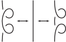
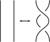
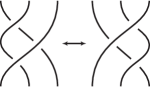
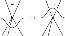
Figure 8.

Lemma 12.1.

The vector $\mathbb{F}_{\mathcal{C}}(G)\in H(G)^{\star}$ is a well-defined isotopy invariant of $G$ preserved under the moves in Figure 8.

Proof.

Independence of $\mathbb{F}_{\mathcal{C}}(G)$ of the choice of the half-edges $e_{v}$ follows from the definition of $H_{v}(G)$. Invariance of $\mathbb{F}_{\mathcal{C}}(G)$ under isotopies of $G$ follows from the sphericity of $\mathcal{C}$.

We claim that, as in Section 3.3, if a $\mathcal{C}$-colored knotted graph $G^{\prime}\subset S^{2}$ is obtained from a $\mathcal{C}$-colored knotted graph $G\subset S^{2}$ through replacement of the color of an edge $e$ by its dual and simultaneous reversion of the orientation of $e$, then the isomorphism $\psi_{X}\colon X\to X^{**}$ of Remark 1.5 (where $X\in\mathrm{Ob}(\mathcal{C})$ is the quasi-color of $e$) induces an isomorphism $\widehat{\psi}\colon H(G)\to H(G^{\prime})$ such that $(\widehat{\psi})^{\star}(\mathbb{F}_{\mathcal{C}}(G^{\prime}))=\mathbb{F}_{\mathcal{C}}(G)$. This claim is verified by comparing the contributions of the vertices and crossings of $G$, $G^{\prime}$ to $\mathbb{F}_{\mathcal{C}}(G)$, $\mathbb{F}_{\mathcal{C}}(G^{\prime})$ respectively. Indeed, without loss of generality, we can assume that $G\subset\mathbb{R}^{2}=S^{2}\setminus\{\infty\}$ and $G$ is generic with respect to the second coordinate on $\mathbb{R}^{2}$. Consider a crossing $x$ of $G$ with over-passing edge $e_{o}$ and under-passing edge $e_{u}$. Applying if necessary an isotopy to $G$ in a neighborhood of $x$, we can assume that $e_{o}$ is directed from top-left to bottom-right. Let $(A,\sigma)\in\mathcal{Z}(\mathcal{C})$ be the color of $e_{o}$ and $X\in\mathrm{Ob}(\mathcal{C})$ be the quasi-color of $e_{u}$. There are four cases to consider depending on the orientation of $e_{u}$ at $x$ (downwards or upwards) and depending on whether we reverse the orientation of $e_{o}$ or $e_{u}$. Assume that $e_{u}$ is directed downwards at $x$, so that the contribution of $x$ to $\mathbb{F}_{\mathcal{C}}(G)$ is

$$\raisebox{-0.45pt}{\scalebox{0.9}{\includegraphics{sigmainv3.eps}}}\;.$$

If $G^{\prime}$ is obtained by reversing $e_{u}$ and replacing its color with the dual object, then the contribution of $x$ to $\mathbb{F}_{\mathcal{C}}(G^{\prime})$ is

$$\raisebox{-0.45pt}{\scalebox{0.9}{\includegraphics{sigmainv4.eps}}}\;.$$

The last equality follows from the definition of $\psi_{X}$ and the formula

$$\sigma_{X}^{-1}=(\widetilde{\mathrm{ev}}_{X}\otimes\mathrm{id}_{{{A}}\otimes X})(\mathrm{id}_{X}\otimes\sigma_{X^{*}}\otimes\mathrm{id}_{X})(\mathrm{id}_{X\otimes{{A}}}\otimes\widetilde{\mathrm{coev}}_{X}).$$

The latter formula can be easily deduced from the naturality of $\sigma$ and Formula (15). Similarly, if $G^{\prime}$ is obtained by reversing $e_{u}$ and replacing its color with the dual object, then the contributions of $x$ to $\mathbb{F}_{\mathcal{C}}(G)$ and $\mathbb{F}_{\mathcal{C}}(G^{\prime})$ are obtained from each other through conjugation by $\psi_{A}$ (to see this, one should use the expression for the dual of a half braiding given in Section 10.2). The case where $e_{u}$ is directed upwards is treated similarly. Combining these local computations, we obtain the required claim.

Consider the second move in Figure 8. Applying if necessary the property of $\mathbb{F}_{\mathcal{C}}$ obtained in the previous paragraph, we can reduce ourselves to the case where both strands are oriented downward. In this case the required identity follows from the definition of $\mathbb{F}_{\mathcal{C}}(G)$. Similarly, to prove the invariance of $\mathbb{F}_{\mathcal{C}}(G)$ under the fourth move, it suffices to consider the case where all edges incident to the vertex are oriented to the left. The required identity follows from the definitions and the properties of $\sigma$. The invariance of $\mathbb{F}_{\mathcal{C}}(G)$ under the third move can be proved similarly treating the crossing point of the two lower branches as a vertex. Finally, the first move expands as a composition of the other moves through pushing the over-passing branch to the left across the rest of the diagram and across the point $\infty\in S^{2}$. ∎

Note that Lemma 4.2 extends mutatis mutandis to $\mathcal{C}$-colored knotted graphs in $S^{2}$.

12.2. Link diagrams

Let $M$ be a compact oriented 3-manifold. Given a s-skeleton $P$ of $M$, that is, a s-skeleton of the pair $(M,\emptyset)$ in the sense of Section 8.1, we can present links in $M$ by diagrams in $P$, see [Tu, Chapter IX]. (Similar presentations can be defined on arbitrary skeletons of $M$, but s-skeletons will be sufficient for our aims.) A link diagram in $P$ is a finite set of loops in $P$ such that:

1. the loops do not meet the vertices of $P$ and meet the edges of $P$ transversely;

2. the loops have only double transversal crossings and self-crossings lying in $\mathrm{Int}(P)=P\setminus P^{(1)}$;

3. at each crossing point of the loops one of the two intersecting branches is distinguished and said to be “lower”, the second branch being “upper”.

The underlying $4$-valent graph of a link diagram is formed by the loops of the diagram with over/under-crossing data forgotten. By abuse of notation, we shall usually denote a link diagram and its underlying graph by the same symbol.

Each link diagram $d$ in $P$ determines a link $\ell_{d}\subset M$ as follows. The orientations of $M$ and $P$ determine a distinguished normal direction on $\mathrm{Int}(P)$ in $M$. Pushing slightly all upper branches of $d$ in $M\setminus P$ in this direction, we transform $d$ into $\ell_{d}$. The underlying loops of $d$ have a well-defined normal line bundle ${b}_{P}(d)$ in $P$; this bundle is defined in the points of $d\cap P^{(1)}$ since, in a neighborhood of any such point, $d$ traverses two regions of $P$ locally forming a 2-disk. The bundle ${b}_{P}(d)$ induces a line subbundle ${b}_{d}$ of the (2-dimensional) normal bundle of $\ell_{d}$ in $M$.

An enriched link diagram in $P$ is a link diagram in $P$ whose loops are equipped with half-integers called pre-twists. The pre-twist of a loop $L$ is required to belong to $\mathbb{Z}$ if the normal line bundle of $L$ in $P$ is trivial and to $\frac{1}{2}+\mathbb{Z}$ otherwise. The pre-twists determine a framing of $\ell_{d}\subset M$ as follows. Twist ${b}_{d}$ around each component of $\ell_{d}$ as many times as the pre-twist of the corresponding loop. (The positive direction of the twist is determined by the orientation of $M$. For instance, a pre-twist of $\frac{1}{2}$ gives rise to a positive half-twist of ${b}_{d}$.) This produces a trivial normal line bundle on $\ell_{d}$. Its non-zero sections yield a framing of $\ell_{d}$.

It is easy to see that every framed link in $M$ may be represented by an enriched link diagram in $P$. Consider the moves $\Omega_{1},\dots,\Omega_{8}$ on enriched link diagrams shown in Figure 9 where the orientation of $M$ corresponds to the right-handed orientation in ${\mathbb{R}}^{3}$. The moves $\Omega_{1},\Omega_{2},\Omega_{3}$ proceed in $\mathrm{Int}(P)$, and $\Omega_{4},\dots,\Omega_{8}$ proceed in a neighborhood of $P^{(1)}$. In Figure 9 the link diagrams on $P$ are drawn in red bold in order to distinguish them from the edges of $P$. The move $\Omega_{1}$ decreases the pre-twist by $1$ and $\Omega_{4}$ increases the pre-twist by $\frac{1}{2}$; the other moves do not change the pre-twists. The move $\Omega_{6}$ has four versions; in the one in Figure 9 we assume that the orientations of the horizontal regions are compatible, i.e., are induced by an orientation of the horizontal plane. If these orientations are incompatible, then the picture must be modified: the overcrossing on the left (or on the right) should be replaced with an undercrossing. The third and fourth versions of $\Omega_{6}$ are obtained from the first two by changing both overcrossings to undercrossings. The move $\Omega_{7}$ has two versions; both apply only when the left horizontal region is oriented counterclockwise. By [Tu], two enriched link diagrams in $P$ represent isotopic framed links if and only if these diagrams may be related by a finite sequence of moves $\Omega_{1}^{\pm 1},\dots,\Omega_{8}^{\pm 1}$ and ambient isotopies in $P$.

Oriented framed links in $M$ can be similarly presented by oriented link diagrams in $P$. These are the (enriched) link diagrams as above formed by oriented loops. Two such diagrams present isotopic oriented framed links if and only if they may be related by the moves in Figure 9 where all strands are oriented (the orientations of the strands must be the same before and after the moves).

\psfrag{T}[Bc][Bc]{\scalebox{1.0}{$\Omega_{1}$}}\psfrag{A}[Bc][Bc]{\scalebox{1.0}{{\color[rgb]{1,0,0}$\mathbf{-1}$}}}\includegraphics{move-omega1.eps}   ,    \psfrag{T}[Bc][Bc]{\scalebox{1.0}{$\Omega_{1}$}}\psfrag{A}[Bc][Bc]{\scalebox{1.0}{{\color[rgb]{1,0,0}$\mathbf{-1}$}}}\psfrag{T}[Bc][Bc]{\scalebox{1.0}{$\Omega_{2}$}}\includegraphics{move-omega2.eps}   ,    \psfrag{T}[Bc][Bc]{\scalebox{1.0}{$\Omega_{1}$}}\psfrag{A}[Bc][Bc]{\scalebox{1.0}{{\color[rgb]{1,0,0}$\mathbf{-1}$}}}\psfrag{T}[Bc][Bc]{\scalebox{1.0}{$\Omega_{2}$}}\psfrag{T}[Bc][Bc]{\scalebox{1.0}{$\Omega_{3}$}}\includegraphics{move-omega3.eps}  ,

\psfrag{T}[Bc][Bc]{\scalebox{1.0}{$\Omega_{1}$}}\psfrag{A}[Bc][Bc]{\scalebox{1.0}{{\color[rgb]{1,0,0}$\mathbf{-1}$}}}\psfrag{T}[Bc][Bc]{\scalebox{1.0}{$\Omega_{2}$}}\psfrag{T}[Bc][Bc]{\scalebox{1.0}{$\Omega_{3}$}}\psfrag{T}[Bc][Bc]{\scalebox{1.0}{$\Omega_{4}$}}\psfrag{h}[Bc][Bc]{\scalebox{0.6}{{\color[rgb]{1,0,0}$\displaystyle\mathbf{\frac{1}{2}}$}}}\includegraphics{move-omega4a.eps} \psfrag{T}[Bc][Bc]{\scalebox{1.0}{$\Omega_{1}$}}\psfrag{A}[Bc][Bc]{\scalebox{1.0}{{\color[rgb]{1,0,0}$\mathbf{-1}$}}}\psfrag{T}[Bc][Bc]{\scalebox{1.0}{$\Omega_{2}$}}\psfrag{T}[Bc][Bc]{\scalebox{1.0}{$\Omega_{3}$}}\psfrag{T}[Bc][Bc]{\scalebox{1.0}{$\Omega_{4}$}}\psfrag{h}[Bc][Bc]{\scalebox{0.6}{{\color[rgb]{1,0,0}$\displaystyle\mathbf{\frac{1}{2}}$}}}\psfrag{T}[Bc][Bc]{\scalebox{1.0}{$\Omega_{5}$}}\includegraphics{move-omega5a.eps}

\psfrag{T}[Bc][Bc]{\scalebox{1.0}{$\Omega_{1}$}}\psfrag{A}[Bc][Bc]{\scalebox{1.0}{{\color[rgb]{1,0,0}$\mathbf{-1}$}}}\psfrag{T}[Bc][Bc]{\scalebox{1.0}{$\Omega_{2}$}}\psfrag{T}[Bc][Bc]{\scalebox{1.0}{$\Omega_{3}$}}\psfrag{T}[Bc][Bc]{\scalebox{1.0}{$\Omega_{4}$}}\psfrag{h}[Bc][Bc]{\scalebox{0.6}{{\color[rgb]{1,0,0}$\displaystyle\mathbf{\frac{1}{2}}$}}}\psfrag{T}[Bc][Bc]{\scalebox{1.0}{$\Omega_{5}$}}\psfrag{T}[Bc][Bc]{\scalebox{1.0}{$\Omega_{6}$}}\includegraphics{move-omega6a.eps} \psfrag{T}[Bc][Bc]{\scalebox{1.0}{$\Omega_{1}$}}\psfrag{A}[Bc][Bc]{\scalebox{1.0}{{\color[rgb]{1,0,0}$\mathbf{-1}$}}}\psfrag{T}[Bc][Bc]{\scalebox{1.0}{$\Omega_{2}$}}\psfrag{T}[Bc][Bc]{\scalebox{1.0}{$\Omega_{3}$}}\psfrag{T}[Bc][Bc]{\scalebox{1.0}{$\Omega_{4}$}}\psfrag{h}[Bc][Bc]{\scalebox{0.6}{{\color[rgb]{1,0,0}$\displaystyle\mathbf{\frac{1}{2}}$}}}\psfrag{T}[Bc][Bc]{\scalebox{1.0}{$\Omega_{5}$}}\psfrag{T}[Bc][Bc]{\scalebox{1.0}{$\Omega_{6}$}}\psfrag{T}[Bc][Bc]{\scalebox{1.0}{$\Omega_{8}$}}\includegraphics{move-omega8a.eps}

\psfrag{T}[Bc][Bc]{\scalebox{1.0}{$\Omega_{1}$}}\psfrag{A}[Bc][Bc]{\scalebox{1.0}{{\color[rgb]{1,0,0}$\mathbf{-1}$}}}\psfrag{T}[Bc][Bc]{\scalebox{1.0}{$\Omega_{2}$}}\psfrag{T}[Bc][Bc]{\scalebox{1.0}{$\Omega_{3}$}}\psfrag{T}[Bc][Bc]{\scalebox{1.0}{$\Omega_{4}$}}\psfrag{h}[Bc][Bc]{\scalebox{0.6}{{\color[rgb]{1,0,0}$\displaystyle\mathbf{\frac{1}{2}}$}}}\psfrag{T}[Bc][Bc]{\scalebox{1.0}{$\Omega_{5}$}}\psfrag{T}[Bc][Bc]{\scalebox{1.0}{$\Omega_{6}$}}\psfrag{T}[Bc][Bc]{\scalebox{1.0}{$\Omega_{8}$}}\psfrag{T}[Bc][Bc]{\scalebox{1.0}{$\Omega_{7.1}$}}\includegraphics{move-omega7a.eps} \psfrag{T}[Bc][Bc]{\scalebox{1.0}{$\Omega_{1}$}}\psfrag{A}[Bc][Bc]{\scalebox{1.0}{{\color[rgb]{1,0,0}$\mathbf{-1}$}}}\psfrag{T}[Bc][Bc]{\scalebox{1.0}{$\Omega_{2}$}}\psfrag{T}[Bc][Bc]{\scalebox{1.0}{$\Omega_{3}$}}\psfrag{T}[Bc][Bc]{\scalebox{1.0}{$\Omega_{4}$}}\psfrag{h}[Bc][Bc]{\scalebox{0.6}{{\color[rgb]{1,0,0}$\displaystyle\mathbf{\frac{1}{2}}$}}}\psfrag{T}[Bc][Bc]{\scalebox{1.0}{$\Omega_{5}$}}\psfrag{T}[Bc][Bc]{\scalebox{1.0}{$\Omega_{6}$}}\psfrag{T}[Bc][Bc]{\scalebox{1.0}{$\Omega_{8}$}}\psfrag{T}[Bc][Bc]{\scalebox{1.0}{$\Omega_{7.1}$}}\psfrag{T}[Bc][Bc]{\scalebox{1.0}{$\Omega_{7.2}$}}\includegraphics{move-omega7b.eps}

Figure 9. Moves $\Omega_{1}-\Omega_{8}$ on link diagrams

12.3. Invariants of links

A component $K$ of a link $L$ in a 3-manifold $M$ is said to be trivial if there is an embedded 2-disk $D\subset M$ such that $K=\partial D=D\cap L$. Consider a pair $(M,L)$, where $M$ is a compact oriented 3-manifold and $L\subset\mathrm{Int}(M)$ is an oriented framed link whose all components are non-trivial and colored by simple objects of $\mathcal{Z}(\mathcal{C})$. We define an invariant $|M,L|_{\mathcal{C}}\in\Bbbk$ as follows. Fix a (finite) representative set $I$ of simple objects of $\mathcal{C}$. Pick a s-skeleton $P$ of $M$ and an oriented enriched link diagram $d$ in $P$ representing $L$. The set ${\widetilde{d}}=P^{(1)}\cup d$ is a graph embedded in $P$ with edges contained either in $P^{(1)}$ or in $d$ and vertices of three types: the vertices of $P^{(1)}$, the points of $P^{(1)}\cap d$, and the crossings of $d$. The assumption that all components of $L$ are non-trivial ensures that every component of ${\widetilde{d}}$ contains at least one vertex, so that ${\widetilde{d}}$ is a graph in the sense of Section 3.1. Cutting out $P$ along ${\widetilde{d}}$, we obtain a compact oriented surface whose components are disks and disks with holes. These components are called the regions of $d$. The set of regions of $d$ is denoted by $\mathrm{Reg}(d)$.

Pick a map $c\colon\mathrm{Reg}(d)\to I$. For any oriented edge $e$ of the graph ${\widetilde{d}}$, we define a $\Bbbk$-module $H_{c}(e)$. If $e\subset P^{(1)}$, then $H_{c}(e)=H(P_{e})$ as in Section 6.3. If $e\subset d$, then there are two regions $r_{-},r_{+}\in\mathrm{Reg}(d)$ adjacent to $e$. We choose notation so that the orientation of $r_{+}$ (resp. $r_{-}$) induces on $e$ the orientation compatible with that of $e$ (resp. opposite to that of $e$):

\psfrag{M}[Bl][Bl]{\scalebox{0.9}{{\color[rgb]{1,0,0}${{A}}$}}}\psfrag{r}[Bc][Bc]{\scalebox{0.9}{$r_{+}$}}\psfrag{v}[Bc][Bc]{\scalebox{0.9}{$r_{-}$}}\psfrag{l}[Bc][Bc]{\scalebox{0.9}{$e$}}\includegraphics{ell-regions.eps} .

Let ${{A}}\in\mathrm{Ob}(\mathcal{C})$ be the quasi-color of the component of $L$ containing $e$. We turn the 3-element set $P_{e}=\{r_{-},e,r_{+}\}$ into a cyclic $\mathcal{C}$-set by providing it with the cyclic order $r_{-}<e<r_{+}<r_{-}$ and with the map to $\mathrm{Ob}(\mathcal{C})\times\{+,-\}$ carrying $r_{\pm}$ to $(c(r_{\pm}),\pm)$ and $e$ to $({{A}},\varepsilon)$, where $\varepsilon=+$ if the orientations of $e$ and $d$ are compatible and $\varepsilon=-$ otherwise. Set

$$H_{c}(e)=H(P_{e})\cong\mathrm{Hom}_{\mathcal{C}}(\mathbb{1},c(r_{-})^{*}\otimes{{A}}^{\varepsilon}\otimes c(r_{+})).$$

It is clear that in both cases $P_{e^{\mathrm{op}}}=(P_{e})^{\mathrm{op}}$. This induces a duality between the modules $H_{c}(e)$, $H_{c}(e^{\mathrm{op}})$ and a contraction $\ast_{e}\colon H_{c}(e)^{\star}\otimes H_{c}(e^{\mathrm{op}})^{\star}\to\Bbbk$.

We now associate to every vertex $x$ of ${\widetilde{d}}$ a certain vector $|x|_{c}$. We distinguish three cases. If $x$ is a vertex of $P^{(1)}$, then as in Section 6.3, the link of $x$ determines a $\mathcal{C}$-colored graph $\Gamma_{x}\subset S^{2}$. Set $|x|_{c}=\mathbb{F}_{\mathcal{C}}(\Gamma_{x})\in H_{c}(\Gamma_{x})^{*}$.

If $x$ is a crossing of $d$, then a neighborhood of $x$ in $P$ looks as follows:

\psfrag{i}[Bc][Bc]{\scalebox{0.9}{$i$}}\psfrag{j}[Bc][Bc]{\scalebox{0.9}{$j$}}\psfrag{k}[Bc][Bc]{\scalebox{0.9}{$k$}}\psfrag{M}[Br][Br]{\scalebox{0.9}{{\color[rgb]{1,0,0}$J$}}}\psfrag{N}[Bl][Bl]{\scalebox{0.9}{{\color[rgb]{1,0,0}$J^{\prime}$}}}\psfrag{l}[Bc][Bc]{\scalebox{0.9}{$l$}}\includegraphics{demi-vert2.eps}

Here $J$ and $J^{\prime}$ are the colors of the strands of $d$ meeting at $x$, and $i,j,k,l\in I$ are the $c$-colors of the regions in $\mathrm{Reg}(d)$ adjacent to $x$. Let $\Gamma_{x}$ be the following $\mathcal{C}$-colored knotted graph in $\mathbb{R}^{2}\subset S^{2}$:

$$\Gamma_{x}=\,\raisebox{-0.45pt}{\scalebox{0.9}{\includegraphics{demi-vert2-inv.eps}}}$$

The orientation (not shown in the picture) of the diagonals is induced by that of $d$. Section 12.1 yields a tensor $|x|_{c}=\mathbb{F}_{\mathcal{C}}(\Gamma_{x})\in H_{c}(\Gamma_{x})^{*}$.

The definition of $|x|_{c}$ in the remaining case $x\in P^{(1)}\cap d$ uses the assumption that the colors of the components of $L$ are simple objects. Since $\Bbbk$ is an algebraically closed field, we can choose for each component of $L$ a square root $\nu_{J}\in\Bbbk$ of the twist scalar $v_{J}\in\Bbbk$ of the color $J$ of this component, see Section 10.1. (At the end, the invariant $|M,L|_{\mathcal{C}}\in\Bbbk$ will be independent of this choice.) A neighborhood of $x\in P^{(1)}\cap d$ in $P$ looks as follows (as usual, the orientation of $M$ is right-handed):

$$\raisebox{-0.45pt}{\scalebox{0.9}{\includegraphics{demi-vert1.eps}}}\,.$$

The skeleton $P$ has 3 regions (possibly coinciding) adjacent to $x$. We denote them $r,r^{-},r^{+}$ so that the strand of $d$ at $x$ goes from $r^{-}$ to $r^{+}$. Let $J$ be the color of this strand. The diagram $d$ has 5 regions adjacent to $x$. We denote their $c$-colors by $i,j,k,l,m$ as in the picture. Let $e_{0}$ be a tangent vector at $x$ directed inside $r$ and let $(e^{\pm}_{1},e^{\pm}_{2})$ be a positive (i.e., positively oriented) basis of the tangent space of $r^{\pm}$ at $x$. Consider the basis $(e_{0},e^{\pm}_{1},e^{\pm}_{2})$ of the tangent space of $M$ at $x$. Set $\varepsilon^{\pm}_{x}=1$ if this basis is positive and $\varepsilon^{\pm}_{x}=-1$ if it is negative. Let $\Gamma_{x}$ be the following $\mathcal{C}$-colored knotted graph in $\mathbb{R}^{2}\subset S^{2}$:

$$\Gamma_{x}=\raisebox{-0.45pt}{\scalebox{0.9}{\includegraphics{demi-vert3-inv.eps}}}$$

where

$$\raisebox{-0.45pt}{\scalebox{0.9}{\includegraphics{demi-vert-choix1.eps}}}=\left\{\begin{array}[]{ll}\raisebox{-0.45pt}{\scalebox{0.9}{\includegraphics{demi-vert-choix1b.eps}}}&\text{if $\varepsilon^{{-}}_{x}=-1$,}\\ \raisebox{-0.45pt}{\scalebox{0.9}{\includegraphics{demi-vert-choix1a.eps}}}&\text{if $\varepsilon^{{-}}_{x}=1$,}\end{array}\right.\quad\raisebox{-0.45pt}{\scalebox{0.9}{\includegraphics{demi-vert-choix2.eps}}}=\left\{\begin{array}[]{ll}\raisebox{-0.45pt}{\scalebox{0.9}{\includegraphics{demi-vert-choix2b.eps}}}&\text{if $\varepsilon^{{+}}_{x}=-1$,}\\ \raisebox{-0.45pt}{\scalebox{0.9}{\includegraphics{demi-vert-choix2a.eps}}}&\text{if $\varepsilon^{{+}}_{x}=1$.}\end{array}\right.$$

The latter pictures determine the orientations of the edges of $\Gamma_{x}$ colored by $i,j,k,l$. The edge of $\Gamma_{x}$ colored by $m$ is directed downward if the orientation of $r$ followed by that of $d$ at $x$ yields the positive orientation of $M$ and upward otherwise. Set

$$\varepsilon_{x}=\frac{\varepsilon^{{-}}_{x}-\varepsilon^{{+}}_{x}}{2}\in\{-1,0,1\}\quad\quad\text{and}\quad\quad|x|_{c}=\nu_{J}^{\varepsilon_{x}}\,\mathbb{F}_{\mathcal{C}}(\Gamma_{x})\in H_{c}(\Gamma_{x})^{\star}.$$

For any vertex $x$ of $\widetilde{d}$, we have $H_{c}(\Gamma_{x})=\otimes_{e}\,H_{c}(e)$, where $e$ runs over the edges of ${\widetilde{d}}$ incident to $x$ and oriented away from $x$. The tensor product $\otimes_{x}\,|x|_{c}$ over all vertices $x$ of ${\widetilde{d}}$ is a vector in $\otimes_{e}\,H_{c}(e)^{\star}$, where $e$ runs over all oriented edges of ${\widetilde{d}}$. Set $\ast_{P}=\otimes_{e}\,\ast_{e}\colon\otimes_{e}\,H_{c}(e)^{\star}\to\Bbbk$.

Let $L_{1},...,L_{N}$ be the components of $L$. Let $J_{q}\in\mathrm{Ob}(\mathcal{Z}(\mathcal{C}))$ be the color of $L_{q}$. Recall the distinguished square root $\nu_{J_{q}}\in\Bbbk$ of the twist scalar $v_{J_{q}}$ of ${J_{q}}$. Let $n_{q}\in\frac{1}{2}\mathbb{Z}$ be the pre-twist of the loop of $d$ representing $L_{q}$, where $q=1,...,N$. Set

$$|M,L|_{\mathcal{C}}=(\dim(\mathcal{C}))^{-|P|}\prod_{q=1}^{N}\nu_{J_{q}}^{2n_{q}}\sum_{c}\left(\prod_{r\in\mathrm{Reg}(d)}\!(\dim c(r))^{\chi(r)}\right){\ast}_{P}(\otimes_{x}\,|x|_{c})\in\Bbbk,$$

where $|P|$ is the number of components of $M\setminus P$, $c$ runs over all maps $\mathrm{Reg}(d)\to I$, and $\chi(r)$ is the Euler characteristic of $r$.

Lemma 12.2.

$|M,L|_{\mathcal{C}}$ is a topological invariant of the pair $(M,L)$ independent of the choice of $I$ and of the choice of square roots of the twist scalars.

Proof.

The independence of $I$ follows from the naturality of $\mathbb{F}_{\mathcal{C}}$ and of the contraction homomorphisms. We prove the independence of the choice of ${\nu_{J_{q}}}$. The term of $|M,L|_{\mathcal{C}}$ determined by a map $\mathrm{Reg}(d)\to I$ is a product of an expression independent of ${\nu_{J_{q}}}$ and $\nu_{J_{q}}^{2n_{q}+s_{q}}$ for $s_{q}=\sum_{x}\varepsilon_{x}$, where $x$ runs over the intersections of the $q$-th component of $d$ with $P^{(1)}$. It suffices to show that $2n_{q}+s_{q}\in 2\mathbb{Z}$. Observe that $\varepsilon_{x}=0$ if the orientations of the regions $r_{-}$ and $r_{+}$ at $x$ are compatible, and $\varepsilon_{x}=\pm 1$ otherwise. Therefore $s_{q}\in 2\mathbb{Z}$ if and only if the normal bundle of the $i$-th component of $d$ in $P$ is trivial. By the definition of a pre-twist, the latter condition holds if and only if $n_{q}\in\mathbb{Z}$. Therefore, $2n_{q}+s_{q}\in 2\mathbb{Z}$ in all cases.

Recall that any two s-skeletons of $M$ can be related by a sequence of Matveev-Piergallini moves. Using $\Omega_{5}^{\pm 1},\Omega_{6}$, and $\Omega_{8}$ we can deform any diagram of $L$ on $P$ away from the place where an MP-move is performed on $P$. Then the same arguments as in the proof of Theorems 5.1 and 6.1 show that $|M,L|_{\mathcal{C}}$ is invariant under the MP-move in question. Therefore we need only to verify that $|M,L|_{\mathcal{C}}$ is invariant under the moves $\Omega_{1},\dots,\Omega_{8}$.

Without loss of generality, we can assume that in the pictures of $\Omega_{1},\Omega_{2},\Omega_{3}$ the orientation of the ambient region corresponds to the counterclockwise orientation of the plane of the picture. For any orientation of the red-bold strand, colored by a simple object $J$ of $\mathcal{Z}(\mathcal{C})$,

\psfrag{M}[Bl][Bl]{\scalebox{0.9}{{\color[rgb]{1,0,0}$J$}}}\psfrag{N}[Br][Br]{\scalebox{0.9}{{\color[rgb]{1,0,0}$J$}}}\psfrag{x}[Bc][Bc]{\scalebox{0.9}{${z}$}}\psfrag{i}[Bc][Bc]{\scalebox{0.9}{$i$}}\psfrag{j}[Bc][Bc]{\scalebox{0.9}{$j$}}\includegraphics{proof-omega1a.eps} $\displaystyle\;\sum_{{z}\in I}\dim({z})$   \psfrag{M}[Bl][Bl]{\scalebox{0.9}{{\color[rgb]{1,0,0}$J$}}}\psfrag{N}[Br][Br]{\scalebox{0.9}{{\color[rgb]{1,0,0}$J$}}}\psfrag{x}[Bc][Bc]{\scalebox{0.9}{${z}$}}\psfrag{i}[Bc][Bc]{\scalebox{0.9}{$i$}}\psfrag{j}[Bc][Bc]{\scalebox{0.9}{$j$}}\includegraphics{proof-omega1b.eps} $\;=\;$ \psfrag{M}[Bl][Bl]{\scalebox{0.9}{{\color[rgb]{1,0,0}$J$}}}\psfrag{N}[Br][Br]{\scalebox{0.9}{{\color[rgb]{1,0,0}$J$}}}\psfrag{x}[Bc][Bc]{\scalebox{0.9}{${z}$}}\psfrag{i}[Bc][Bc]{\scalebox{0.9}{$i$}}\psfrag{j}[Bc][Bc]{\scalebox{0.9}{$j$}}\includegraphics{proof-omega1c.eps} $\;=\,\displaystyle v_{J}$  \psfrag{M}[Bl][Bl]{\scalebox{0.9}{{\color[rgb]{1,0,0}$J$}}}\psfrag{N}[Br][Br]{\scalebox{0.9}{{\color[rgb]{1,0,0}$J$}}}\psfrag{x}[Bc][Bc]{\scalebox{0.9}{${z}$}}\psfrag{i}[Bc][Bc]{\scalebox{0.9}{$i$}}\psfrag{j}[Bc][Bc]{\scalebox{0.9}{$j$}}\includegraphics{proof-omega1d.eps}  .

The arrow indicates that we compute the contribution of the picture (the curl) to the state sum. The dotted arc indicates the tensor contraction of the vector spaces corresponding to the endpoints of the arc. The equalities follow respectively from Lemma 4.2.c and the definition of the twist scalar $v_{J}$ (if the red-bold strand is oriented upward, one should also use the equality $v_{J^{*}}=v_{J}$). Taking into account the normalization factor $\prod_{q}\nu_{q}^{2n_{q}}$ and the additional pre-twist $-1$ introduced by $\Omega_{1}$, we conclude that $|M,L|_{\mathcal{C}}$ is invariant under $\Omega_{1}$.

For any orientations of the red-bold strands (colored by simple objects of $\mathcal{Z}(\mathcal{C})$),

\psfrag{M}[Br][Br]{\scalebox{0.9}{{\color[rgb]{1,0,0}$J$}}}\psfrag{N}[Bl][Bl]{\scalebox{0.9}{{\color[rgb]{1,0,0}$J^{\prime}$}}}\psfrag{x}[Bc][Bc]{\scalebox{0.9}{${z}$}}\psfrag{i}[Bc][Bc]{\scalebox{0.9}{$i$}}\psfrag{j}[Bc][Bc]{\scalebox{0.9}{$j$}}\psfrag{k}[Bc][Bc]{\scalebox{0.9}{$k$}}\psfrag{l}[Bl][Bl]{\scalebox{0.9}{$l$}}\includegraphics{proof-omega2a.eps} $\displaystyle\sum_{{z}\in I}\dim({z})$   \psfrag{M}[Br][Br]{\scalebox{0.9}{{\color[rgb]{1,0,0}$J$}}}\psfrag{N}[Bl][Bl]{\scalebox{0.9}{{\color[rgb]{1,0,0}$J^{\prime}$}}}\psfrag{x}[Bc][Bc]{\scalebox{0.9}{${z}$}}\psfrag{i}[Bc][Bc]{\scalebox{0.9}{$i$}}\psfrag{j}[Bc][Bc]{\scalebox{0.9}{$j$}}\psfrag{k}[Bc][Bc]{\scalebox{0.9}{$k$}}\psfrag{l}[Bl][Bl]{\scalebox{0.9}{$l$}}\includegraphics{proof-omega2b.eps} $\displaystyle\;=\sum_{{z}\in I}\dim({z})$   \psfrag{M}[Br][Br]{\scalebox{0.9}{{\color[rgb]{1,0,0}$J$}}}\psfrag{N}[Bl][Bl]{\scalebox{0.9}{{\color[rgb]{1,0,0}$J^{\prime}$}}}\psfrag{x}[Bc][Bc]{\scalebox{0.9}{${z}$}}\psfrag{i}[Bc][Bc]{\scalebox{0.9}{$i$}}\psfrag{j}[Bc][Bc]{\scalebox{0.9}{$j$}}\psfrag{k}[Bc][Bc]{\scalebox{0.9}{$k$}}\psfrag{l}[Bl][Bl]{\scalebox{0.9}{$l$}}\includegraphics{proof-omega2c.eps} $\;=\;$ \psfrag{M}[Br][Br]{\scalebox{0.9}{{\color[rgb]{1,0,0}$J$}}}\psfrag{N}[Bl][Bl]{\scalebox{0.9}{{\color[rgb]{1,0,0}$J^{\prime}$}}}\psfrag{x}[Bc][Bc]{\scalebox{0.9}{${z}$}}\psfrag{i}[Bc][Bc]{\scalebox{0.9}{$i$}}\psfrag{j}[Bc][Bc]{\scalebox{0.9}{$j$}}\psfrag{k}[Bc][Bc]{\scalebox{0.9}{$k$}}\psfrag{l}[Bl][Bl]{\scalebox{0.9}{$l$}}\includegraphics{proof-omega2d.eps}

$\;=\;$ \psfrag{M}[Br][Br]{\scalebox{0.9}{{\color[rgb]{1,0,0}$J$}}}\psfrag{N}[Bl][Bl]{\scalebox{0.9}{{\color[rgb]{1,0,0}$J^{\prime}$}}}\psfrag{x}[Bc][Bc]{\scalebox{0.9}{${z}$}}\psfrag{i}[Bc][Bc]{\scalebox{0.9}{$i$}}\psfrag{j}[Bc][Bc]{\scalebox{0.9}{$j$}}\psfrag{k}[Bc][Bc]{\scalebox{0.9}{$k$}}\psfrag{l}[Bl][Bl]{\scalebox{0.9}{$l$}}\includegraphics{proof-omega2e.eps} $\;=\;\displaystyle\delta_{k,l}$   \psfrag{M}[Br][Br]{\scalebox{0.9}{{\color[rgb]{1,0,0}$J$}}}\psfrag{N}[Bl][Bl]{\scalebox{0.9}{{\color[rgb]{1,0,0}$J^{\prime}$}}}\psfrag{x}[Bc][Bc]{\scalebox{0.9}{${z}$}}\psfrag{i}[Bc][Bc]{\scalebox{0.9}{$i$}}\psfrag{j}[Bc][Bc]{\scalebox{0.9}{$j$}}\psfrag{k}[Bc][Bc]{\scalebox{0.9}{$k$}}\psfrag{l}[Bl][Bl]{\scalebox{0.9}{$l$}}\psfrag{j}[Bc][Bc]{\scalebox{0.9}{$k$}}\includegraphics{proof-omega1d.eps}   \psfrag{M}[Br][Br]{\scalebox{0.9}{{\color[rgb]{1,0,0}$J$}}}\psfrag{N}[Bl][Bl]{\scalebox{0.9}{{\color[rgb]{1,0,0}$J^{\prime}$}}}\psfrag{x}[Bc][Bc]{\scalebox{0.9}{${z}$}}\psfrag{i}[Bc][Bc]{\scalebox{0.9}{$i$}}\psfrag{j}[Bc][Bc]{\scalebox{0.9}{$j$}}\psfrag{k}[Bc][Bc]{\scalebox{0.9}{$k$}}\psfrag{l}[Bl][Bl]{\scalebox{0.9}{$l$}}\psfrag{j}[Bc][Bc]{\scalebox{0.9}{$k$}}\psfrag{i}[Bc][Bc]{\scalebox{0.9}{$k$}}\psfrag{j}[Bc][Bc]{\scalebox{0.9}{$j$}}\includegraphics{proof-omega1d.eps}    \psfrag{M}[Br][Br]{\scalebox{0.9}{{\color[rgb]{1,0,0}$J$}}}\psfrag{N}[Bl][Bl]{\scalebox{0.9}{{\color[rgb]{1,0,0}$J^{\prime}$}}}\psfrag{x}[Bc][Bc]{\scalebox{0.9}{${z}$}}\psfrag{i}[Bc][Bc]{\scalebox{0.9}{$i$}}\psfrag{j}[Bc][Bc]{\scalebox{0.9}{$j$}}\psfrag{k}[Bc][Bc]{\scalebox{0.9}{$k$}}\psfrag{l}[Bl][Bl]{\scalebox{0.9}{$l$}}\psfrag{j}[Bc][Bc]{\scalebox{0.9}{$k$}}\psfrag{i}[Bc][Bc]{\scalebox{0.9}{$k$}}\psfrag{j}[Bc][Bc]{\scalebox{0.9}{$j$}}\psfrag{i}[Bc][Bc]{\scalebox{0.9}{$i$}}\includegraphics{proof-omega2f.eps}  .

The first two equalities follow respectively from Claims (d) and (c) of Lemma 4.2. The third equality follows from Lemma 12.1. We conclude that $|M,L|_{\mathcal{C}}$ is invariant under $\Omega_{2}$. The invariance under $\Omega_{3}$ is verified similarly.

Below we verify the invariance of $|M,L|_{\mathcal{C}}$ under the moves $\Omega_{4},\dots\Omega_{8}$ for a certain orientation of the link diagram. The proof of the invariance for the opposite orientation of a component of the diagram can be obtained by repeating exactly the same arguments but using everywhere the opposite orientation of the relevant edges of the $\mathcal{C}$-colored knotted graphs. In particular, the tensors associated with all vertices are represented by the same graphs with opposite orientation of the appropriate red-bold edges. For the tensors associated with the crossings, this follows directly from the definitions. For the tensors associated with the vertices of $P^{(1)}\cap d$, we use that

\psfrag{M}[Br][Br]{\scalebox{0.9}{{\color[rgb]{1,0,0}$J$}}}\includegraphics{proof-link-orient1b.eps} $\quad=\quad$ \psfrag{M}[Br][Br]{\scalebox{0.9}{{\color[rgb]{1,0,0}$J$}}}\includegraphics{proof-link-orient2b.eps} $\quad=\;\nu_{J}^{-2}\quad$ \psfrag{M}[Br][Br]{\scalebox{0.9}{{\color[rgb]{1,0,0}$J$}}}\includegraphics{proof-link-orient3b.eps}  .

and

\psfrag{M}[Br][Br]{\scalebox{0.9}{{\color[rgb]{1,0,0}$J$}}}\includegraphics{proof-link-orient1.eps} $\quad=\quad$ \psfrag{M}[Br][Br]{\scalebox{0.9}{{\color[rgb]{1,0,0}$J$}}}\includegraphics{proof-link-orient2.eps} $\quad=\;\nu_{J}^{2}\quad$ \psfrag{M}[Br][Br]{\scalebox{0.9}{{\color[rgb]{1,0,0}$J$}}}\includegraphics{proof-link-orient3.eps}  .

For example, we have

\psfrag{M}[Bc][Bc]{\scalebox{0.9}{{\color[rgb]{1,0,0}$J$}}}\psfrag{i}[Bc][Bc]{\scalebox{0.9}{$i$}}\psfrag{j}[Bc][Bc]{\scalebox{0.9}{$j$}}\psfrag{k}[Bc][Bc]{\scalebox{0.9}{$k$}}\psfrag{l}[Bc][Bc]{\scalebox{0.9}{$l$}}\psfrag{m}[Bc][Bc]{\scalebox{0.9}{$m$}}\includegraphics{proof-link-orient-ex1.eps} $\quad\nu_{J}^{\frac{-1-1}{2}}\,$ \psfrag{M}[Bc][Bc]{\scalebox{0.9}{{\color[rgb]{1,0,0}$J$}}}\psfrag{i}[Bc][Bc]{\scalebox{0.9}{$i$}}\psfrag{j}[Bc][Bc]{\scalebox{0.9}{$j$}}\psfrag{k}[Bc][Bc]{\scalebox{0.9}{$k$}}\psfrag{l}[Bc][Bc]{\scalebox{0.9}{$l$}}\psfrag{m}[Bc][Bc]{\scalebox{0.9}{$m$}}\includegraphics{proof-link-orient-ex2.eps}

and

\psfrag{M}[Bc][Bc]{\scalebox{0.9}{{\color[rgb]{1,0,0}$J$}}}\psfrag{X}[Br][Br]{\scalebox{1.11}{$\nu_{J}^{\frac{1+1}{2}}$}}\psfrag{Y}[Br][Br]{\scalebox{1.11}{$=\,\nu_{J}^{-1}$}}\psfrag{i}[Bc][Bc]{\scalebox{0.9}{$i$}}\psfrag{j}[Bc][Bc]{\scalebox{0.9}{$j$}}\psfrag{k}[Bc][Bc]{\scalebox{0.9}{$k$}}\psfrag{l}[Bc][Bc]{\scalebox{0.9}{$l$}}\psfrag{m}[Bc][Bc]{\scalebox{0.9}{$m$}}\includegraphics{proof-link-orient-ex1b.eps}  .

The last graph differs from the graph obtained in the previous picture only by the orientation of the red-bold edge.

Let us now verify the invariance of $|M,L|_{\mathcal{C}}$ under the moves $\Omega_{4}-\Omega_{8}$ for a certain orientation of the s-skeleton and of the link diagram. We begin with $\Omega_{4}$, $\Omega_{5}$, and $\Omega_{8}$. In these computations, the (unique) red-bold strand is colored with a simple object $J$ of $\mathcal{Z}(\mathcal{C})$. We have

\psfrag{M}[Bc][Bc]{\scalebox{0.9}{{\color[rgb]{1,0,0}$J$}}}\psfrag{x}[Bc][Bc]{\scalebox{0.9}{${z}$}}\psfrag{i}[Bc][Bc]{\scalebox{0.9}{$i$}}\psfrag{j}[Bc][Bc]{\scalebox{0.9}{$j$}}\psfrag{k}[Bc][Bc]{\scalebox{0.9}{$k$}}\psfrag{l}[Bc][Bc]{\scalebox{0.9}{$l$}}\psfrag{m}[Bc][Bc]{\scalebox{0.9}{$m$}}\includegraphics{proof-omega4a.eps}

$\displaystyle\nu_{J}^{\frac{-1-1}{2}}\,\nu_{J}^{\frac{1-1}{2}}\;\sum_{{z}\in I}\dim({z})\;$ \psfrag{M}[Bc][Bc]{\scalebox{0.9}{{\color[rgb]{1,0,0}$J$}}}\psfrag{x}[Bc][Bc]{\scalebox{0.9}{${z}$}}\psfrag{i}[Bc][Bc]{\scalebox{0.9}{$i$}}\psfrag{j}[Bc][Bc]{\scalebox{0.9}{$j$}}\psfrag{k}[Bc][Bc]{\scalebox{0.9}{$k$}}\psfrag{l}[Bc][Bc]{\scalebox{0.9}{$l$}}\psfrag{m}[Bc][Bc]{\scalebox{0.9}{$m$}}\includegraphics{proof-omega4b.eps}

$\displaystyle=\,\nu_{J}^{-1}\;\sum_{{z}\in I}\dim({z})\;$ \psfrag{M}[Bc][Bc]{\scalebox{0.9}{{\color[rgb]{1,0,0}$J$}}}\psfrag{x}[Bc][Bc]{\scalebox{0.9}{${z}$}}\psfrag{i}[Bc][Bc]{\scalebox{0.9}{$i$}}\psfrag{j}[Bc][Bc]{\scalebox{0.9}{$j$}}\psfrag{k}[Bc][Bc]{\scalebox{0.9}{$k$}}\psfrag{l}[Bc][Bc]{\scalebox{0.9}{$l$}}\psfrag{m}[Bc][Bc]{\scalebox{0.9}{$m$}}\includegraphics{proof-omega4c.eps}

$\displaystyle=\,\nu_{J}^{-1}\;\sum_{{z}\in I}\dim({z})\;$ \psfrag{M}[Bc][Bc]{\scalebox{0.9}{{\color[rgb]{1,0,0}$J$}}}\psfrag{x}[Bc][Bc]{\scalebox{0.9}{${z}$}}\psfrag{i}[Bc][Bc]{\scalebox{0.9}{$i$}}\psfrag{j}[Bc][Bc]{\scalebox{0.9}{$j$}}\psfrag{k}[Bc][Bc]{\scalebox{0.9}{$k$}}\psfrag{l}[Bc][Bc]{\scalebox{0.9}{$l$}}\psfrag{m}[Bc][Bc]{\scalebox{0.9}{$m$}}\includegraphics{proof-omega4d.eps}

$\displaystyle=\,\nu_{J}^{-1}\;$ \psfrag{M}[Bc][Bc]{\scalebox{0.9}{{\color[rgb]{1,0,0}$J$}}}\psfrag{x}[Bc][Bc]{\scalebox{0.9}{${z}$}}\psfrag{i}[Bc][Bc]{\scalebox{0.9}{$i$}}\psfrag{j}[Bc][Bc]{\scalebox{0.9}{$j$}}\psfrag{k}[Bc][Bc]{\scalebox{0.9}{$k$}}\psfrag{l}[Bc][Bc]{\scalebox{0.9}{$l$}}\psfrag{m}[Bc][Bc]{\scalebox{0.9}{$m$}}\includegraphics{proof-omega4e.eps} $\displaystyle=\,\nu_{J}^{-1}\;$ \psfrag{M}[Bc][Bc]{\scalebox{0.9}{{\color[rgb]{1,0,0}$J$}}}\psfrag{x}[Bc][Bc]{\scalebox{0.9}{${z}$}}\psfrag{i}[Bc][Bc]{\scalebox{0.9}{$i$}}\psfrag{j}[Bc][Bc]{\scalebox{0.9}{$j$}}\psfrag{k}[Bc][Bc]{\scalebox{0.9}{$k$}}\psfrag{l}[Bc][Bc]{\scalebox{0.9}{$l$}}\psfrag{m}[Bc][Bc]{\scalebox{0.9}{$m$}}\includegraphics{proof-omega4f.eps}

All these equalities except the penultimate one follow from Lemma 12.1; the penultimate equality follows from Lemma 4.2. By definition,

\psfrag{M}[Bc][Bc]{\scalebox{0.9}{{\color[rgb]{1,0,0}$J$}}}\psfrag{x}[Bc][Bc]{\scalebox{0.9}{${z}$}}\psfrag{i}[Bc][Bc]{\scalebox{0.9}{$i$}}\psfrag{j}[Bc][Bc]{\scalebox{0.9}{$j$}}\psfrag{k}[Bc][Bc]{\scalebox{0.9}{$k$}}\psfrag{l}[Bc][Bc]{\scalebox{0.9}{$l$}}\psfrag{m}[Bc][Bc]{\scalebox{0.9}{$m$}}\includegraphics{proof-omega4g.eps} $\displaystyle\;\nu_{J}^{\frac{-1+1}{2}}\;$ \psfrag{M}[Bc][Bc]{\scalebox{0.9}{{\color[rgb]{1,0,0}$J$}}}\psfrag{x}[Bc][Bc]{\scalebox{0.9}{${z}$}}\psfrag{i}[Bc][Bc]{\scalebox{0.9}{$i$}}\psfrag{j}[Bc][Bc]{\scalebox{0.9}{$j$}}\psfrag{k}[Bc][Bc]{\scalebox{0.9}{$k$}}\psfrag{l}[Bc][Bc]{\scalebox{0.9}{$l$}}\psfrag{m}[Bc][Bc]{\scalebox{0.9}{$m$}}\includegraphics{proof-omega4h.eps}  .

Taking into account the normalization factor $\prod_{q}\nu_{q}^{2n_{q}}$ and the additional pre-twist $\frac{1}{2}$ introduced by $\Omega_{4}$, we conclude that $|M,L|_{\mathcal{C}}$ is invariant under $\Omega_{4}$.

Next, we have

\psfrag{M}[Bc][Bc]{\scalebox{0.9}{{\color[rgb]{1,0,0}$J$}}}\psfrag{x}[Bc][Bc]{\scalebox{0.9}{${z}$}}\psfrag{i}[Bc][Bc]{\scalebox{0.9}{$i$}}\psfrag{j}[Bc][Bc]{\scalebox{0.9}{$j$}}\psfrag{k}[Bc][Bc]{\scalebox{0.9}{$k$}}\psfrag{l}[Bc][Bc]{\scalebox{0.9}{$l$}}\psfrag{m}[Bc][Bc]{\scalebox{0.9}{$m$}}\includegraphics{proof-omega5a.eps}

$\displaystyle\nu_{J}^{\frac{1-1}{2}}\,\nu_{J}^{\frac{1-1}{2}}\;\sum_{{z}\in I}\dim({z})$ \psfrag{M}[Bc][Bc]{\scalebox{0.9}{{\color[rgb]{1,0,0}$J$}}}\psfrag{x}[Bc][Bc]{\scalebox{0.9}{${z}$}}\psfrag{i}[Bc][Bc]{\scalebox{0.9}{$i$}}\psfrag{j}[Bc][Bc]{\scalebox{0.9}{$j$}}\psfrag{k}[Bc][Bc]{\scalebox{0.9}{$k$}}\psfrag{l}[Bc][Bc]{\scalebox{0.9}{$l$}}\psfrag{m}[Bc][Bc]{\scalebox{0.9}{$m$}}\includegraphics{proof-omega5b.eps} $\;=\;$ \psfrag{M}[Bc][Bc]{\scalebox{0.9}{{\color[rgb]{1,0,0}$J$}}}\psfrag{x}[Bc][Bc]{\scalebox{0.9}{${z}$}}\psfrag{i}[Bc][Bc]{\scalebox{0.9}{$i$}}\psfrag{j}[Bc][Bc]{\scalebox{0.9}{$j$}}\psfrag{k}[Bc][Bc]{\scalebox{0.9}{$k$}}\psfrag{l}[Bc][Bc]{\scalebox{0.9}{$l$}}\psfrag{m}[Bc][Bc]{\scalebox{0.9}{$m$}}\includegraphics{proof-omega5c.eps}

$\;=\;$ \psfrag{M}[Bc][Bc]{\scalebox{0.9}{{\color[rgb]{1,0,0}$J$}}}\psfrag{x}[Bc][Bc]{\scalebox{0.9}{${z}$}}\psfrag{i}[Bc][Bc]{\scalebox{0.9}{$i$}}\psfrag{j}[Bc][Bc]{\scalebox{0.9}{$j$}}\psfrag{k}[Bc][Bc]{\scalebox{0.9}{$k$}}\psfrag{l}[Bc][Bc]{\scalebox{0.9}{$l$}}\psfrag{m}[Bc][Bc]{\scalebox{0.9}{$m$}}\includegraphics{proof-omega5d.eps} $\;=\;\delta_{i,k}\;$ \psfrag{M}[Bc][Bc]{\scalebox{0.9}{{\color[rgb]{1,0,0}$J$}}}\psfrag{x}[Bc][Bc]{\scalebox{0.9}{${z}$}}\psfrag{i}[Bc][Bc]{\scalebox{0.9}{$i$}}\psfrag{j}[Bc][Bc]{\scalebox{0.9}{$j$}}\psfrag{k}[Bc][Bc]{\scalebox{0.9}{$k$}}\psfrag{l}[Bc][Bc]{\scalebox{0.9}{$l$}}\psfrag{m}[Bc][Bc]{\scalebox{0.9}{$m$}}\includegraphics{proof-omega5e.eps}  .

The right-hand side is the contribution to the state sum of the following piece of the diagram:

\psfrag{M}[Bc][Bc]{\scalebox{0.9}{{\color[rgb]{1,0,0}$J$}}}\psfrag{x}[Bc][Bc]{\scalebox{0.9}{${z}$}}\psfrag{i}[Bc][Bc]{\scalebox{0.9}{$i$}}\psfrag{j}[Bc][Bc]{\scalebox{0.9}{$j$}}\psfrag{k}[Bc][Bc]{\scalebox{0.9}{$k$}}\psfrag{l}[Bc][Bc]{\scalebox{0.9}{$l$}}\psfrag{m}[Bc][Bc]{\scalebox{0.9}{$m$}}\includegraphics{proof-omega5f.eps}  .

Therefore the state sum is invariant under $\Omega_{5}$.

Next, we have

\psfrag{x}[Bc][Bc]{\scalebox{0.9}{${z}$}}\psfrag{i}[Bc][Bc]{\scalebox{0.9}{$i$}}\psfrag{j}[Bc][Bc]{\scalebox{0.9}{$j$}}\psfrag{k}[Bc][Bc]{\scalebox{0.9}{$k$}}\psfrag{l}[Bc][Bc]{\scalebox{0.9}{$l$}}\psfrag{m}[Bc][Bc]{\scalebox{0.9}{$m$}}\psfrag{n}[Bc][Bc]{\scalebox{0.9}{$n$}}\psfrag{p}[Bc][Bc]{\scalebox{0.9}{$p$}}\psfrag{q}[Bc][Bc]{\scalebox{0.9}{$q$}}\includegraphics{proof-omega8a.eps}

$\displaystyle\nu_{J}^{\frac{1-1}{2}}\,\nu_{J}^{\frac{1-1}{2}}\;\sum_{{z}\in I}\dim({z})$ \psfrag{x}[Bc][Bc]{\scalebox{0.9}{${z}$}}\psfrag{i}[Bc][Bc]{\scalebox{0.9}{$i$}}\psfrag{j}[Bc][Bc]{\scalebox{0.9}{$j$}}\psfrag{k}[Bc][Bc]{\scalebox{0.9}{$k$}}\psfrag{l}[Bc][Bc]{\scalebox{0.9}{$l$}}\psfrag{m}[Bc][Bc]{\scalebox{0.9}{$m$}}\psfrag{n}[Bc][Bc]{\scalebox{0.9}{$n$}}\psfrag{p}[Bc][Bc]{\scalebox{0.9}{$p$}}\psfrag{q}[Bc][Bc]{\scalebox{0.9}{$q$}}\includegraphics{proof-omega8b.eps}

$=\;$ \psfrag{x}[Bc][Bc]{\scalebox{0.9}{${z}$}}\psfrag{i}[Bc][Bc]{\scalebox{0.9}{$i$}}\psfrag{j}[Bc][Bc]{\scalebox{0.9}{$j$}}\psfrag{k}[Bc][Bc]{\scalebox{0.9}{$k$}}\psfrag{l}[Bc][Bc]{\scalebox{0.9}{$l$}}\psfrag{m}[Bc][Bc]{\scalebox{0.9}{$m$}}\psfrag{n}[Bc][Bc]{\scalebox{0.9}{$n$}}\psfrag{p}[Bc][Bc]{\scalebox{0.9}{$p$}}\psfrag{q}[Bc][Bc]{\scalebox{0.9}{$q$}}\includegraphics{proof-omega8c.eps} $\;=\;$ \psfrag{x}[Bc][Bc]{\scalebox{0.9}{${z}$}}\psfrag{i}[Bc][Bc]{\scalebox{0.9}{$i$}}\psfrag{j}[Bc][Bc]{\scalebox{0.9}{$j$}}\psfrag{k}[Bc][Bc]{\scalebox{0.9}{$k$}}\psfrag{l}[Bc][Bc]{\scalebox{0.9}{$l$}}\psfrag{m}[Bc][Bc]{\scalebox{0.9}{$m$}}\psfrag{n}[Bc][Bc]{\scalebox{0.9}{$n$}}\psfrag{p}[Bc][Bc]{\scalebox{0.9}{$p$}}\psfrag{q}[Bc][Bc]{\scalebox{0.9}{$q$}}\includegraphics{proof-omega8d.eps}

$\displaystyle=\nu_{J}^{\frac{1-1}{2}}$ \psfrag{x}[Bc][Bc]{\scalebox{0.9}{${z}$}}\psfrag{i}[Bc][Bc]{\scalebox{0.9}{$i$}}\psfrag{j}[Bc][Bc]{\scalebox{0.9}{$j$}}\psfrag{k}[Bc][Bc]{\scalebox{0.9}{$k$}}\psfrag{l}[Bc][Bc]{\scalebox{0.9}{$l$}}\psfrag{m}[Bc][Bc]{\scalebox{0.9}{$m$}}\psfrag{n}[Bc][Bc]{\scalebox{0.9}{$n$}}\psfrag{p}[Bc][Bc]{\scalebox{0.9}{$p$}}\psfrag{q}[Bc][Bc]{\scalebox{0.9}{$q$}}\includegraphics{proof-omega8e.eps} \psfrag{x}[Bc][Bc]{\scalebox{0.9}{${z}$}}\psfrag{i}[Bc][Bc]{\scalebox{0.9}{$i$}}\psfrag{j}[Bc][Bc]{\scalebox{0.9}{$j$}}\psfrag{k}[Bc][Bc]{\scalebox{0.9}{$k$}}\psfrag{l}[Bc][Bc]{\scalebox{0.9}{$l$}}\psfrag{m}[Bc][Bc]{\scalebox{0.9}{$m$}}\psfrag{n}[Bc][Bc]{\scalebox{0.9}{$n$}}\psfrag{p}[Bc][Bc]{\scalebox{0.9}{$p$}}\psfrag{q}[Bc][Bc]{\scalebox{0.9}{$q$}}\includegraphics{proof-omega8f.eps}

Therefore the state sum is invariant under $\Omega_{8}$.

Consider now the moves $\Omega_{6}$ and $\Omega_{7}$. We assume that the two red-bold strands are colored with simple objects $J$, $J^{\prime}$ of $\mathcal{Z}(\mathcal{C})$. We have

\psfrag{M}[Bl][Bl]{\scalebox{0.9}{{\color[rgb]{1,0,0}$J$}}}\psfrag{N}[Bl][Bl]{\scalebox{0.9}{{\color[rgb]{1,0,0}$J^{\prime}$}}}\psfrag{x}[Bc][Bc]{\scalebox{0.9}{${z}$}}\psfrag{i}[Bc][Bc]{\scalebox{0.9}{$i$}}\psfrag{j}[Bc][Bc]{\scalebox{0.9}{$j$}}\psfrag{k}[Bc][Bc]{\scalebox{0.9}{$k$}}\psfrag{l}[Bc][Bc]{\scalebox{0.9}{$l$}}\psfrag{m}[Bc][Bc]{\scalebox{0.9}{$m$}}\psfrag{n}[Bc][Bc]{\scalebox{0.9}{$n$}}\psfrag{p}[Bc][Bc]{\scalebox{0.9}{$p$}}\includegraphics{proof-omega6a.eps}

$\displaystyle\nu_{J}^{\frac{1-1}{2}}\,\nu_{J^{\prime}}^{\frac{1-1}{2}}\;\sum_{{z}\in I}\dim({z})$   \psfrag{M}[Bl][Bl]{\scalebox{0.9}{{\color[rgb]{1,0,0}$J$}}}\psfrag{N}[Bl][Bl]{\scalebox{0.9}{{\color[rgb]{1,0,0}$J^{\prime}$}}}\psfrag{x}[Bc][Bc]{\scalebox{0.9}{${z}$}}\psfrag{i}[Bc][Bc]{\scalebox{0.9}{$i$}}\psfrag{j}[Bc][Bc]{\scalebox{0.9}{$j$}}\psfrag{k}[Bc][Bc]{\scalebox{0.9}{$k$}}\psfrag{l}[Bc][Bc]{\scalebox{0.9}{$l$}}\psfrag{m}[Bc][Bc]{\scalebox{0.9}{$m$}}\psfrag{n}[Bc][Bc]{\scalebox{0.9}{$n$}}\psfrag{p}[Bc][Bc]{\scalebox{0.9}{$p$}}\includegraphics{proof-omega6b.eps}

$=\;$ \psfrag{M}[Bl][Bl]{\scalebox{0.9}{{\color[rgb]{1,0,0}$J$}}}\psfrag{N}[Bl][Bl]{\scalebox{0.9}{{\color[rgb]{1,0,0}$J^{\prime}$}}}\psfrag{x}[Bc][Bc]{\scalebox{0.9}{${z}$}}\psfrag{i}[Bc][Bc]{\scalebox{0.9}{$i$}}\psfrag{j}[Bc][Bc]{\scalebox{0.9}{$j$}}\psfrag{k}[Bc][Bc]{\scalebox{0.9}{$k$}}\psfrag{l}[Bc][Bc]{\scalebox{0.9}{$l$}}\psfrag{m}[Bc][Bc]{\scalebox{0.9}{$m$}}\psfrag{n}[Bc][Bc]{\scalebox{0.9}{$n$}}\psfrag{p}[Bc][Bc]{\scalebox{0.9}{$p$}}\includegraphics{proof-omega6c.eps} $\;=\;$ \psfrag{M}[Bl][Bl]{\scalebox{0.9}{{\color[rgb]{1,0,0}$J$}}}\psfrag{N}[Bl][Bl]{\scalebox{0.9}{{\color[rgb]{1,0,0}$J^{\prime}$}}}\psfrag{x}[Bc][Bc]{\scalebox{0.9}{${z}$}}\psfrag{i}[Bc][Bc]{\scalebox{0.9}{$i$}}\psfrag{j}[Bc][Bc]{\scalebox{0.9}{$j$}}\psfrag{k}[Bc][Bc]{\scalebox{0.9}{$k$}}\psfrag{l}[Bc][Bc]{\scalebox{0.9}{$l$}}\psfrag{m}[Bc][Bc]{\scalebox{0.9}{$m$}}\psfrag{n}[Bc][Bc]{\scalebox{0.9}{$n$}}\psfrag{p}[Bc][Bc]{\scalebox{0.9}{$p$}}\includegraphics{proof-omega6d.eps}

$\displaystyle=\nu_{J}^{\frac{1-1}{2}}\,\nu_{J^{\prime}}^{\frac{1-1}{2}}\;\sum_{{z}\in I}\dim({z})$   \psfrag{M}[Bl][Bl]{\scalebox{0.9}{{\color[rgb]{1,0,0}$J$}}}\psfrag{N}[Bl][Bl]{\scalebox{0.9}{{\color[rgb]{1,0,0}$J^{\prime}$}}}\psfrag{x}[Bc][Bc]{\scalebox{0.9}{${z}$}}\psfrag{i}[Bc][Bc]{\scalebox{0.9}{$i$}}\psfrag{j}[Bc][Bc]{\scalebox{0.9}{$j$}}\psfrag{k}[Bc][Bc]{\scalebox{0.9}{$k$}}\psfrag{l}[Bc][Bc]{\scalebox{0.9}{$l$}}\psfrag{m}[Bc][Bc]{\scalebox{0.9}{$m$}}\psfrag{n}[Bc][Bc]{\scalebox{0.9}{$n$}}\psfrag{p}[Bc][Bc]{\scalebox{0.9}{$p$}}\includegraphics{proof-omega6e.eps}

\psfrag{M}[Bl][Bl]{\scalebox{0.9}{{\color[rgb]{1,0,0}$J$}}}\psfrag{N}[Bl][Bl]{\scalebox{0.9}{{\color[rgb]{1,0,0}$J^{\prime}$}}}\psfrag{x}[Bc][Bc]{\scalebox{0.9}{${z}$}}\psfrag{i}[Bc][Bc]{\scalebox{0.9}{$i$}}\psfrag{j}[Bc][Bc]{\scalebox{0.9}{$j$}}\psfrag{k}[Bc][Bc]{\scalebox{0.9}{$k$}}\psfrag{l}[Bc][Bc]{\scalebox{0.9}{$l$}}\psfrag{m}[Bc][Bc]{\scalebox{0.9}{$m$}}\psfrag{n}[Bc][Bc]{\scalebox{0.9}{$n$}}\psfrag{p}[Bc][Bc]{\scalebox{0.9}{$p$}}\includegraphics{proof-omega6f.eps}  .

Therefore the state sum is invariant under $\Omega_{6}$.

We verify the invariance for $\Omega_{7.1}$ (the case of $\Omega_{7.2}$ is similar). We have

\psfrag{M}[Bl][Bl]{\scalebox{0.9}{{\color[rgb]{1,0,0}$J$}}}\psfrag{N}[Bl][Bl]{\scalebox{0.9}{{\color[rgb]{1,0,0}$J^{\prime}$}}}\psfrag{x}[Bc][Bc]{\scalebox{0.9}{${z}$}}\psfrag{i}[Bc][Bc]{\scalebox{0.9}{$i$}}\psfrag{j}[Bc][Bc]{\scalebox{0.9}{$j$}}\psfrag{k}[Bc][Bc]{\scalebox{0.9}{$k$}}\psfrag{l}[Bc][Bc]{\scalebox{0.9}{$l$}}\psfrag{m}[Bc][Bc]{\scalebox{0.9}{$m$}}\psfrag{n}[Bc][Bc]{\scalebox{0.9}{$n$}}\psfrag{p}[Bc][Bc]{\scalebox{0.9}{$p$}}\psfrag{q}[Bc][Bc]{\scalebox{0.9}{$q$}}\includegraphics{proof-omega7a.eps}

$\displaystyle\nu_{J}^{\frac{-1+1}{2}}\,\nu_{J^{\prime}}^{\frac{1-1}{2}}\;\sum_{{z}\in I}\dim({z})$   \psfrag{M}[Bl][Bl]{\scalebox{0.9}{{\color[rgb]{1,0,0}$J$}}}\psfrag{N}[Bl][Bl]{\scalebox{0.9}{{\color[rgb]{1,0,0}$J^{\prime}$}}}\psfrag{x}[Bc][Bc]{\scalebox{0.9}{${z}$}}\psfrag{i}[Bc][Bc]{\scalebox{0.9}{$i$}}\psfrag{j}[Bc][Bc]{\scalebox{0.9}{$j$}}\psfrag{k}[Bc][Bc]{\scalebox{0.9}{$k$}}\psfrag{l}[Bc][Bc]{\scalebox{0.9}{$l$}}\psfrag{m}[Bc][Bc]{\scalebox{0.9}{$m$}}\psfrag{n}[Bc][Bc]{\scalebox{0.9}{$n$}}\psfrag{p}[Bc][Bc]{\scalebox{0.9}{$p$}}\psfrag{q}[Bc][Bc]{\scalebox{0.9}{$q$}}\includegraphics{proof-omega7b.eps}

$=\;\displaystyle\sum_{{z}\in I}\dim({z})$ \psfrag{M}[Bl][Bl]{\scalebox{0.9}{{\color[rgb]{1,0,0}$J$}}}\psfrag{N}[Bl][Bl]{\scalebox{0.9}{{\color[rgb]{1,0,0}$J^{\prime}$}}}\psfrag{x}[Bc][Bc]{\scalebox{0.9}{${z}$}}\psfrag{i}[Bc][Bc]{\scalebox{0.9}{$i$}}\psfrag{j}[Bc][Bc]{\scalebox{0.9}{$j$}}\psfrag{k}[Bc][Bc]{\scalebox{0.9}{$k$}}\psfrag{l}[Bc][Bc]{\scalebox{0.9}{$l$}}\psfrag{m}[Bc][Bc]{\scalebox{0.9}{$m$}}\psfrag{n}[Bc][Bc]{\scalebox{0.9}{$n$}}\psfrag{p}[Bc][Bc]{\scalebox{0.9}{$p$}}\psfrag{q}[Bc][Bc]{\scalebox{0.9}{$q$}}\includegraphics{proof-omega7c.eps}

$=\;$ \psfrag{M}[Bl][Bl]{\scalebox{0.9}{{\color[rgb]{1,0,0}$J$}}}\psfrag{N}[Bl][Bl]{\scalebox{0.9}{{\color[rgb]{1,0,0}$J^{\prime}$}}}\psfrag{x}[Bc][Bc]{\scalebox{0.9}{${z}$}}\psfrag{i}[Bc][Bc]{\scalebox{0.9}{$i$}}\psfrag{j}[Bc][Bc]{\scalebox{0.9}{$j$}}\psfrag{k}[Bc][Bc]{\scalebox{0.9}{$k$}}\psfrag{l}[Bc][Bc]{\scalebox{0.9}{$l$}}\psfrag{m}[Bc][Bc]{\scalebox{0.9}{$m$}}\psfrag{n}[Bc][Bc]{\scalebox{0.9}{$n$}}\psfrag{p}[Bc][Bc]{\scalebox{0.9}{$p$}}\psfrag{q}[Bc][Bc]{\scalebox{0.9}{$q$}}\includegraphics{proof-omega7d.eps} $\;\,=\,\;$ \psfrag{M}[Bl][Bl]{\scalebox{0.9}{{\color[rgb]{1,0,0}$J$}}}\psfrag{N}[Bl][Bl]{\scalebox{0.9}{{\color[rgb]{1,0,0}$J^{\prime}$}}}\psfrag{x}[Bc][Bc]{\scalebox{0.9}{${z}$}}\psfrag{i}[Bc][Bc]{\scalebox{0.9}{$i$}}\psfrag{j}[Bc][Bc]{\scalebox{0.9}{$j$}}\psfrag{k}[Bc][Bc]{\scalebox{0.9}{$k$}}\psfrag{l}[Bc][Bc]{\scalebox{0.9}{$l$}}\psfrag{m}[Bc][Bc]{\scalebox{0.9}{$m$}}\psfrag{n}[Bc][Bc]{\scalebox{0.9}{$n$}}\psfrag{p}[Bc][Bc]{\scalebox{0.9}{$p$}}\psfrag{q}[Bc][Bc]{\scalebox{0.9}{$q$}}\includegraphics{proof-omega7e.eps} $\;\,=$ \psfrag{M}[Bl][Bl]{\scalebox{0.9}{{\color[rgb]{1,0,0}$J$}}}\psfrag{N}[Bl][Bl]{\scalebox{0.9}{{\color[rgb]{1,0,0}$J^{\prime}$}}}\psfrag{x}[Bc][Bc]{\scalebox{0.9}{${z}$}}\psfrag{i}[Bc][Bc]{\scalebox{0.9}{$i$}}\psfrag{j}[Bc][Bc]{\scalebox{0.9}{$j$}}\psfrag{k}[Bc][Bc]{\scalebox{0.9}{$k$}}\psfrag{l}[Bc][Bc]{\scalebox{0.9}{$l$}}\psfrag{m}[Bc][Bc]{\scalebox{0.9}{$m$}}\psfrag{n}[Bc][Bc]{\scalebox{0.9}{$n$}}\psfrag{p}[Bc][Bc]{\scalebox{0.9}{$p$}}\psfrag{q}[Bc][Bc]{\scalebox{0.9}{$q$}}\includegraphics{proof-omega7f.eps}

$=\displaystyle\nu_{J}^{\frac{-1+1}{2}}\,\nu_{J^{\prime}}^{\frac{1-1}{2}}$ \psfrag{M}[Bl][Bl]{\scalebox{0.9}{{\color[rgb]{1,0,0}$J$}}}\psfrag{N}[Bl][Bl]{\scalebox{0.9}{{\color[rgb]{1,0,0}$J^{\prime}$}}}\psfrag{x}[Bc][Bc]{\scalebox{0.9}{${z}$}}\psfrag{i}[Bc][Bc]{\scalebox{0.9}{$i$}}\psfrag{j}[Bc][Bc]{\scalebox{0.9}{$j$}}\psfrag{k}[Bc][Bc]{\scalebox{0.9}{$k$}}\psfrag{l}[Bc][Bc]{\scalebox{0.9}{$l$}}\psfrag{m}[Bc][Bc]{\scalebox{0.9}{$m$}}\psfrag{n}[Bc][Bc]{\scalebox{0.9}{$n$}}\psfrag{p}[Bc][Bc]{\scalebox{0.9}{$p$}}\psfrag{q}[Bc][Bc]{\scalebox{0.9}{$q$}}\includegraphics{proof-omega7g.eps} \psfrag{M}[Bl][Bl]{\scalebox{0.9}{{\color[rgb]{1,0,0}$J$}}}\psfrag{N}[Bl][Bl]{\scalebox{0.9}{{\color[rgb]{1,0,0}$J^{\prime}$}}}\psfrag{x}[Bc][Bc]{\scalebox{0.9}{${z}$}}\psfrag{i}[Bc][Bc]{\scalebox{0.9}{$i$}}\psfrag{j}[Bc][Bc]{\scalebox{0.9}{$j$}}\psfrag{k}[Bc][Bc]{\scalebox{0.9}{$k$}}\psfrag{l}[Bc][Bc]{\scalebox{0.9}{$l$}}\psfrag{m}[Bc][Bc]{\scalebox{0.9}{$m$}}\psfrag{n}[Bc][Bc]{\scalebox{0.9}{$n$}}\psfrag{p}[Bc][Bc]{\scalebox{0.9}{$p$}}\psfrag{q}[Bc][Bc]{\scalebox{0.9}{$q$}}\includegraphics{proof-omega7h.eps}

Therefore the state sum is invariant under $\Omega_{7}$.

The invariance of $|M,L|_{\mathcal{C}}$ under the moves $\Omega_{4}-\Omega_{8}$ with other orientations of the s-skeleton can be verified similarly. As above, this verification is easy for $\Omega_{5}$ and $\Omega_{6}$ but longer for the other moves. However, having verified this invariance for $\Omega_{5}$ and $\Omega_{6}$, we can prove that $|M,L|_{\mathcal{C}}$ does not depend on the orientation of the s-skeleton $P$. Then the invariance for the other moves follows from the special cases considered above. To prove our claim, it is enough to prove the invariance of $|M,L|_{\mathcal{C}}$ under reversion of the orientation in an arbitrary region, $X$, of $P$. Applying bubble moves $T_{4}^{{}^{\prime\prime}}$ (see Figure 4) at the boundary of $X$, then using $\Omega_{5}$ to push the newly attached disks near the crossings and using $\Omega_{6}$ to pull the crossings into these disks, we can reduce the claim to the case where $X$ contains no crossings of the diagram (note that all these transformations keep $|M,L|_{\mathcal{C}}$). Then $X$ meets the link diagram in several disjoint embedded arcs. Similarly, applying bubble moves $T_{4}^{{}^{\prime\prime}}$ and then lune moves $\mathcal{L}^{\pm 1}$ (see Figure 7) to push the newly attached disks between the arcs of the diagram in $X$, we can reduce the claim to the case where the diagram meets the disk $X$ along a single embedded arc. Finally, applying the moves $(T^{2,1})^{-1}$ (see Figure 6) to $P$ outside the diagram, we can reduce the claim to the case where $X$ has only two vertices in $P$ as in the picture below. There are two cases to consider, depending on whether or not this arc arrives and leaves in the same direction:

  and   

Let us check that the two orientations of the disk do contribute similarly to the state sum. In the first case, we have

\psfrag{M}[Bl][Bl]{\scalebox{0.9}{{\color[rgb]{1,0,0}$J$}}}\psfrag{x}[Bc][Bc]{\scalebox{0.9}{$x$}}\psfrag{i}[Bc][Bc]{\scalebox{0.9}{$i$}}\psfrag{j}[Bc][Bc]{\scalebox{0.9}{$j$}}\psfrag{y}[Bc][Bc]{\scalebox{0.9}{$y$}}\includegraphics{proof-orient1.eps}

$\displaystyle\nu_{J}^{\frac{\varepsilon_{x}^{-}+1}{2}}\,\nu_{J}^{\frac{-1-\varepsilon_{y}^{+}}{2}}\;\sum_{i,j\in I}\dim(i)\dim(j)$   \psfrag{M}[Bl][Bl]{\scalebox{0.9}{{\color[rgb]{1,0,0}$J$}}}\psfrag{x}[Bc][Bc]{\scalebox{0.9}{$x$}}\psfrag{i}[Bc][Bc]{\scalebox{0.9}{$i$}}\psfrag{j}[Bc][Bc]{\scalebox{0.9}{$j$}}\psfrag{y}[Bc][Bc]{\scalebox{0.9}{$y$}}\includegraphics{proof-orient1c.eps}

$=\displaystyle\nu_{J}^{\frac{\varepsilon_{x}^{-}-\varepsilon_{y}^{+}}{2}}\;$ \psfrag{M}[Bl][Bl]{\scalebox{0.9}{{\color[rgb]{1,0,0}$J$}}}\psfrag{x}[Bc][Bc]{\scalebox{0.9}{$x$}}\psfrag{i}[Bc][Bc]{\scalebox{0.9}{$i$}}\psfrag{j}[Bc][Bc]{\scalebox{0.9}{$j$}}\psfrag{y}[Bc][Bc]{\scalebox{0.9}{$y$}}\includegraphics{proof-orient1d.eps} XXXXXXXXXXXXXXXXXX

$=\displaystyle\nu_{J}^{\frac{\varepsilon_{x}^{-}-1}{2}}\,\nu_{J}^{\frac{+1-\varepsilon_{y}^{+}}{2}}\;\sum_{i,j\in I}\dim(i)\dim(j)$   \psfrag{M}[Bl][Bl]{\scalebox{0.9}{{\color[rgb]{1,0,0}$J$}}}\psfrag{x}[Bc][Bc]{\scalebox{0.9}{$x$}}\psfrag{i}[Bc][Bc]{\scalebox{0.9}{$i$}}\psfrag{j}[Bc][Bc]{\scalebox{0.9}{$j$}}\psfrag{y}[Bc][Bc]{\scalebox{0.9}{$y$}}\includegraphics{proof-orient1e.eps}

\psfrag{M}[Bl][Bl]{\scalebox{0.9}{{\color[rgb]{1,0,0}$J$}}}\psfrag{x}[Bc][Bc]{\scalebox{0.9}{$x$}}\psfrag{i}[Bc][Bc]{\scalebox{0.9}{$i$}}\psfrag{j}[Bc][Bc]{\scalebox{0.9}{$j$}}\psfrag{y}[Bc][Bc]{\scalebox{0.9}{$y$}}\includegraphics{proof-orient1b.eps}

In the second case, we have

\psfrag{M}[Bl][Bl]{\scalebox{0.9}{{\color[rgb]{1,0,0}$J$}}}\psfrag{x}[Bc][Bc]{\scalebox{0.9}{$x$}}\psfrag{i}[Bc][Bc]{\scalebox{0.9}{$i$}}\psfrag{j}[Bc][Bc]{\scalebox{0.9}{$j$}}\psfrag{y}[Bc][Bc]{\scalebox{0.9}{$y$}}\includegraphics{proof-orient2.eps}

$\displaystyle\nu_{J}^{\frac{\varepsilon_{x}^{-}+1}{2}}\,\nu_{J}^{\frac{1-\varepsilon_{y}^{+}}{2}}\;\sum_{i,j\in I}\dim(i)\dim(j)$   \psfrag{M}[Bl][Bl]{\scalebox{0.9}{{\color[rgb]{1,0,0}$J$}}}\psfrag{x}[Bc][Bc]{\scalebox{0.9}{$x$}}\psfrag{i}[Bc][Bc]{\scalebox{0.9}{$i$}}\psfrag{j}[Bc][Bc]{\scalebox{0.9}{$j$}}\psfrag{y}[Bc][Bc]{\scalebox{0.9}{$y$}}\includegraphics{proof-orient2c.eps}

$=\displaystyle\nu_{J}^{1+\frac{\varepsilon_{x}^{-}-\varepsilon_{y}^{+}}{2}}\;\sum_{i,j\in I}\dim(i)\dim(j)$   \psfrag{M}[Bl][Bl]{\scalebox{0.9}{{\color[rgb]{1,0,0}$J$}}}\psfrag{x}[Bc][Bc]{\scalebox{0.9}{$x$}}\psfrag{i}[Bc][Bc]{\scalebox{0.9}{$i$}}\psfrag{j}[Bc][Bc]{\scalebox{0.9}{$j$}}\psfrag{y}[Bc][Bc]{\scalebox{0.9}{$y$}}\includegraphics{proof-orient2d.eps}

$=\displaystyle\nu_{J}^{1+\frac{\varepsilon_{x}^{-}-\varepsilon_{y}^{+}}{2}}\;\sum_{i,j\in I}\dim(i)\dim(j)\;$ \psfrag{M}[Bl][Bl]{\scalebox{0.9}{{\color[rgb]{1,0,0}$J$}}}\psfrag{x}[Bc][Bc]{\scalebox{0.9}{$x$}}\psfrag{i}[Bc][Bc]{\scalebox{0.9}{$i$}}\psfrag{j}[Bc][Bc]{\scalebox{0.9}{$j$}}\psfrag{y}[Bc][Bc]{\scalebox{0.9}{$y$}}\includegraphics{proof-orient2e.eps}

$=\displaystyle\nu_{J}^{1+\frac{\varepsilon_{x}^{-}-\varepsilon_{y}^{+}}{2}}\;\sum_{j\in I}\dim(j)$   \psfrag{M}[Bl][Bl]{\scalebox{0.9}{{\color[rgb]{1,0,0}$J$}}}\psfrag{x}[Bc][Bc]{\scalebox{0.9}{$x$}}\psfrag{i}[Bc][Bc]{\scalebox{0.9}{$i$}}\psfrag{j}[Bc][Bc]{\scalebox{0.9}{$j$}}\psfrag{y}[Bc][Bc]{\scalebox{0.9}{$y$}}\includegraphics{proof-orient2f.eps}

$=\displaystyle\nu_{J}^{1+\frac{\varepsilon_{x}^{-}-\varepsilon_{y}^{+}}{2}}$   \psfrag{M}[Bl][Bl]{\scalebox{0.9}{{\color[rgb]{1,0,0}$J$}}}\psfrag{x}[Bc][Bc]{\scalebox{0.9}{$x$}}\psfrag{i}[Bc][Bc]{\scalebox{0.9}{$i$}}\psfrag{j}[Bc][Bc]{\scalebox{0.9}{$j$}}\psfrag{y}[Bc][Bc]{\scalebox{0.9}{$y$}}\includegraphics{proof-orient2g.eps}   $=\displaystyle\nu_{J}^{-1+\frac{\varepsilon_{x}^{-}-\varepsilon_{y}^{+}}{2}}$   \psfrag{M}[Bl][Bl]{\scalebox{0.9}{{\color[rgb]{1,0,0}$J$}}}\psfrag{x}[Bc][Bc]{\scalebox{0.9}{$x$}}\psfrag{i}[Bc][Bc]{\scalebox{0.9}{$i$}}\psfrag{j}[Bc][Bc]{\scalebox{0.9}{$j$}}\psfrag{y}[Bc][Bc]{\scalebox{0.9}{$y$}}\includegraphics{proof-orient2gb.eps}

$=\displaystyle\nu_{J}^{-1+\frac{\varepsilon_{x}^{-}-\varepsilon_{y}^{+}}{2}}\;\sum_{i,j\in I}\dim(i)\dim(j)$   \psfrag{M}[Bl][Bl]{\scalebox{0.9}{{\color[rgb]{1,0,0}$J$}}}\psfrag{x}[Bc][Bc]{\scalebox{0.9}{$x$}}\psfrag{i}[Bc][Bc]{\scalebox{0.9}{$i$}}\psfrag{j}[Bc][Bc]{\scalebox{0.9}{$j$}}\psfrag{y}[Bc][Bc]{\scalebox{0.9}{$y$}}\includegraphics{proof-orient2j.eps}

$=\displaystyle\nu_{J}^{-1+\frac{\varepsilon_{x}^{-}-\varepsilon_{y}^{+}}{2}}\;\sum_{i,j\in I}\dim(i)\dim(j)$   \psfrag{M}[Bl][Bl]{\scalebox{0.9}{{\color[rgb]{1,0,0}$J$}}}\psfrag{x}[Bc][Bc]{\scalebox{0.9}{$x$}}\psfrag{i}[Bc][Bc]{\scalebox{0.9}{$i$}}\psfrag{j}[Bc][Bc]{\scalebox{0.9}{$j$}}\psfrag{y}[Bc][Bc]{\scalebox{0.9}{$y$}}\includegraphics{proof-orient2i.eps}

$=\displaystyle\nu_{J}^{\frac{\varepsilon_{x}^{-}-1}{2}}\,\nu_{J}^{\frac{-1-\varepsilon_{y}^{+}}{2}}\;\sum_{i,j\in I}\dim(i)\dim(j)$   \psfrag{M}[Bl][Bl]{\scalebox{0.9}{{\color[rgb]{1,0,0}$J$}}}\psfrag{x}[Bc][Bc]{\scalebox{0.9}{$x$}}\psfrag{i}[Bc][Bc]{\scalebox{0.9}{$i$}}\psfrag{j}[Bc][Bc]{\scalebox{0.9}{$j$}}\psfrag{y}[Bc][Bc]{\scalebox{0.9}{$y$}}\includegraphics{proof-orient2h.eps}

\psfrag{M}[Bl][Bl]{\scalebox{0.9}{{\color[rgb]{1,0,0}$J$}}}\psfrag{x}[Bc][Bc]{\scalebox{0.9}{$x$}}\psfrag{i}[Bc][Bc]{\scalebox{0.9}{$i$}}\psfrag{j}[Bc][Bc]{\scalebox{0.9}{$j$}}\psfrag{y}[Bc][Bc]{\scalebox{0.9}{$y$}}\includegraphics{proof-orient2b.eps}

This concludes the proof of Lemma 12.2. ∎

12.4. The case of arbitrary links

We extend the invariant $|M,L|_{\mathcal{C}}$ of links without trivial components in a compact oriented 3-manifold $M$ (see Lemma 12.2) to arbitrary links in $M$. Consider an oriented framed link $L\subset\mathrm{Int}(M)$ whose components are colored by simple objects of $\mathcal{Z}(\mathcal{C})$. Let $L_{1},\ldots,L_{k}$ be the trivial components of $L$, and let $\widetilde{L}$ be the sublink of $L$ formed by all the other components. For $i=1,\ldots,k$, let $J_{i}$ be the object of $\mathcal{Z}(\mathcal{C})$ coloring $L_{i}$ and let $f_{i}\in\mathbb{Z}$ be the framing number of $L_{i}$ (defined as in the standard case of knots in the 3-sphere). Set

$$|M,L|_{\mathcal{C}}=|M,\widetilde{L}|_{\mathcal{C}}\,\prod_{i=1}^{k}v_{J_{i}}^{f_{i}}\dim(J_{i})\in\Bbbk.$$

Theorem 12.3.

$|M,L|_{\mathcal{C}}$ is a topological invariant of the pair $(M,L)$.

This theorem directly follows from Lemma 12.2.

The invariant $|M,L|_{\mathcal{C}}$ can be computed via the same formula as in Section 12.3 applied to an arbitrary s-skeleton $P$ of $M$ and an oriented enriched link diagram $d$ in $P$ representing $L$ such that every component of $d$ has a self-crossing or meets the 1-skeleton of $P$.

12.5. Remarks

(1) Since all objects of $\mathcal{Z}(\mathcal{C})$ are direct sums of simple objects, the invariant $|M,L|_{\mathcal{C}}$ extends by linearity to arbitrary colors of the components of $L$.

(2) Theorem 11.1 directly extends to 3- manifolds with links, see Formula (18) in Section 13.5.

12.6. A special case

It is obvious that for $L=\emptyset$, we have $|M,L|_{\mathcal{C}}=|M|_{\mathcal{C}}$, where $|M|_{\mathcal{C}}\in\Bbbk$ is the invariant defined for closed $M$ in Section 5 and generalized to compact $M$ in Section 9.2. We obtain a similar formula for any $\mathcal{Z}(\mathcal{C})$-colored framed oriented link $L$ lying in a 3-ball in $M$. Denote by $L^{\prime}$ the $\mathcal{Z}(\mathcal{C})$-colored framed oriented link in $S^{3}$ obtained by cutting out the ball containing $L$ from $M$ and embedding this ball - with $L$ inside - in $S^{3}$. The embedding in question should be orientation-preserving.

Lemma 12.4.

$|M,L|_{\mathcal{C}}=|M|_{\mathcal{C}}\,F_{\mathcal{Z}(\mathcal{C})}(L^{\prime})$.

Proof.

Pick an s-skeleton $P$ of $M$ and a diagram $d$ of $L$ contained in a region $r$ of $P$. Inserting if necessary small curls in $d$, we can assume that $d$ has at least one self-crossing and all pre-twists of $d$ are equal to zero. Denote the underlying ($4$-valent) graph of $d$ by ${\underline{d}}$. Applying if necessary $\Omega_{2}$ to $d$ in $r$, we can ensure that ${\underline{d}}$ is connected and all its edges have distinct endpoints. Then all regions of $d$ are disks except the “exterior region” $r_{0}$ of $d$ in $r$, which is an annulus. Let $R_{1}$ be the set of the disk regions of $d$ contained in $r$ and $R_{2}$ be the set of all other disk regions of $d$. Thus, $\mathrm{Reg}(d)=R_{1}\amalg R_{2}\amalg\{r_{0}\}$.

Since $P^{(1)}\cap{d}=\emptyset$, the scalar ${\ast}_{P}(\otimes_{x}\,|x|_{c})\in\Bbbk$ in the definition of $|M,L|_{\mathcal{C}}$ expands as a product of two scalars $t^{c}_{1},t^{c}_{2}\in\Bbbk$. The scalar $t^{c}_{1}$ (resp. $t^{c}_{2}$) is obtained from the tensor associated with the vertices of $P^{(1)}$ (resp. ${\underline{d}}$) through the tensor contraction associated with the edges of $P^{(1)}$ (resp. ${\underline{d}}$). Each $t^{c}_{k}$ is determined by $i=c(r_{0})\in I$ and the map $c_{k}=c|_{R_{k}}\colon R_{k}\to I$. We therefore denote $t^{c}_{k}$ by $t^{i,c_{k}}$. We have

$$|M,L|_{\mathcal{C}}=(\dim(\mathcal{C}))^{-|P|}\sum_{i\in I}\sum_{\begin{subarray}{c}c\colon\mathrm{Reg}(d)\to I\\ c(r_{0})=i\end{subarray}}\,\,\left(\prod_{r\in R_{1}\cup R_{2}}\!\dim c(r)\right)\,t^{c}_{1}t^{c}_{2}$$

$$=(\dim(\mathcal{C}))^{-|P|}\sum_{i\in I}\sum_{c_{1}\colon R_{1}\to I}\left(\prod_{r\in R_{1}}\!\dim c_{1}(r)\right)t^{i,c_{1}}\sum_{c_{2}\colon R_{2}\to I}\left(\prod_{r\in R_{2}}\!\dim c_{2}(r)\right)t^{i,c_{2}}.$$

Below we prove that for all $i\in I$,

(16) $$\sum_{c\colon R_{1}\to I}\left(\prod_{r\in R_{1}}\!\dim c(r)\right)t^{i,c}=\dim(i)\,F_{\mathcal{Z}(\mathcal{C})}(L^{\prime}).$$

Substituting this in the expression for $|M,L|_{\mathcal{C}}$ above, we obtain that

$$|M,L|_{\mathcal{C}}=(\dim(\mathcal{C}))^{-|P|}\sum_{i\in I}\sum_{c\colon R_{2}\to I}\left(\prod_{r\in R_{2}}\!\dim c(r)\right)t^{i,c_{2}}\dim(i)\,F_{\mathcal{Z}(\mathcal{C})}(L^{\prime})$$

$$=|M|_{\mathcal{C}}\,F_{\mathcal{Z}(\mathcal{C})}(L^{\prime}).$$

To prove (16), we need to study the graph $\underline{d}$ in more detail. Let $N\geq 1$ be the number of vertices of $\underline{d}$ (i.e., the number of crossings of $d$). Since the graph $\underline{d}$ is 4-valent, it has $2N$ edges. A computation of the Euler characteristic of $r$ shows that $\underline{d}$ splits $r$ into $N+1$ disk regions and the exterior region $r_{0}$. The diagram ${d}$ also determines a graph ${d}^{*}\subset r$ as follows. Fix a point in each region of $d$ in $r$ called the center of the region. These $N+2$ points are the vertices of ${d}^{*}$. Every edge $e$ of ${\underline{d}}$ determines a dual edge $e^{*}$ of ${d}^{*}$ which connects the centers of the two regions adjacent to $e$, meets the interior of $e$ transversely in one point, and is disjoint from ${\underline{d}}$ otherwise. Note that the two regions adjacent to $e$ are always distinct so that the edges of $d^{*}$ are not loops. We choose the edges of ${d}^{*}$ so that they meet only in common vertices. The vertex of ${d}^{*}$ represented by the center of $r_{0}$ is denoted $O$.

By a subgraph of a graph $G$ we mean a graph formed by some vertices and edges of $G$. A subgraph $F$ of $G$ is full if all vertices of $G$ are vertices of $F$. A maximal tree in $G$ is a full subgraph of $G$ which is a tree. Each subgraph $F$ of ${\underline{d}}$ determines a full subgraph $F^{*}$ of ${d}^{*}$ whose edges are dual to the edges of $\underline{d}$ not belonging to $F$. Clearly, $F\cap F^{*}=\emptyset$. If $F$ is a maximal tree in ${\underline{d}}$, then $F^{*}$ is a maximal tree in ${d}^{*}$. Indeed, since every component of $r\setminus F^{*}$ contains a vertex of $\underline{d}$ and any two vertices of $\underline{d}$ can be related by a path in $F\subset r\setminus F^{*}$, the set $r\setminus F^{*}$ is connected. Hence $F^{*}$ is a forest with $N+2$ vertices and $2N-(N-1)=N+1$ edges. Such a forest is necessarily a tree.

Let $e_{1},\ldots,e_{2N}$ be the edges of $\underline{d}$ enumerated so that the following conditions are met. For $k=1,\ldots,2N$, set $F_{k}=\cup_{l=1}^{k}e_{l}\subset\underline{d}$ and observe that $F^{*}_{k}$ is the full subgraph of $d^{*}$ with edges $e_{k+1}^{*},\ldots,e_{2N}^{*}$. We require that (a) the graph $F_{N-1}$ is a maximal tree in $\underline{d}$ and (b) for all $k=N,\ldots,2N$, the graph $F_{k-1}^{*}$ has a 1-valent vertex distinct from $O$ and incident to $e_{k}^{*}$. It is easy to choose $e_{1},\ldots,e_{N-1}$ to ensure (a). We explain now how to choose $e_{k}$ with $k\geq N$ to ensure (b). For $k=N$, pick a 1-valent vertex $v_{N}$ of the maximal tree $F_{N-1}^{*}\subset d^{*}$ distinct from $O$. (Such a vertex exists because a tree having at least one edge necessarily has $\geq 2$ vertices of valency 1.) Let $e_{N}$ be the edge of $\underline{d}$ such that $e^{*}_{N}$ is the edge of $F_{N-1}^{*}$ adjacent to $v_{N}$. The graph $F_{N}^{*}$ is obtained from $F_{N-1}^{*}$ by removing $e^{*}_{N}$ (keeping all the vertices). Clearly, $F_{N}^{*}$ is a disjoint union of the isolated vertex $v_{N}$ and a tree with $N+1$ vertices. We choose $e_{N+1}$ so that $e^{*}_{N+1}$ is the edge of the latter tree adjacent to a 1-valent vertex $v_{N+1}\neq O$. Continuing by induction we obtain that the graph $F_{k}^{*}$ constructed at the $k$-th step consists of isolated vertices $v_{N},\ldots,v_{k}$ and a tree with $2N+1-k$ vertices. We choose $e_{k+1}$ so that $e^{*}_{k+1}$ is the edge of the latter tree adjacent to a 1-valent vertex $v_{k+1}\neq O$. This process stops at $k=2N$ because the graph $F_{2N}^{*}$ has only isolated vertices.

We can now prove (16). Recall that the term $t^{i,c}$ is obtained by placing a small colored tetrahedron-type graph in every crossing of $d$, taking the tensor product of the associated $\mathbb{F}_{\mathcal{Z}(\mathcal{C})}$-invariants, and tensor contracting this product along the edges of $\underline{d}$. The colors of the edges of these tetrahedron-type graphs are determined by $i,c$, and the given coloring of the link components. We shall perform the tensor contraction at one edge at a time following the order of the edges $e_{1},\ldots,e_{2N}$ fixed above. Condition (a) shows that for $k=1,\ldots,N-1$, the $k$-th tensor contraction involves two different pieces of the diagram so that we can apply Claim (d) of Lemma 4.2. At each of these $N-1$ steps, the tensor contraction of the tensor product of two $\mathbb{F}_{\mathcal{Z}(\mathcal{C})}$-invariants yields the $\mathbb{F}_{\mathcal{Z}(\mathcal{C})}$-invariant of a “fused” diagram. For $k\geq N$, the endpoint $v_{k}$ of $e^{*}_{k}$ is the center of a disk region, $V_{k}\subset r$, of $d$ adjacent to the edge $e_{k}$. Note that all other sides of $V_{k}$ (i.e., all other edges of $d$ adjacent to $V_{k}$) must have appeared at the previous steps among $e_{1},\ldots,e_{k-1}$. This follows from the fact that neither of the edges $e_{k+1}^{*},\ldots,e_{2N}^{*}$ is adjacent to $v_{k}$. Therefore the fusions corresponding to all sides of $V_{k}$ except $e_{k}$ have been done before the $k$-th step. The tetrahedron-type graph associated with a vertex of $V_{k}$ has a side in $V_{k}$; under the fusions in question, these sides are united into a single arc labeled with $c(V_{k})$. This shows that the $k$-th tensor contraction involves two vertices of the same connected piece of the diagram. We apply Claim (c) of Lemma 4.2 where the roles of $i,u,v$ are played respectively by $c(V_{k})$ and the endpoints of $e_{k}$ (here we use that all edges of $\underline{d}$ have distinct endpoints). After fusion along $e_{k}$ our diagram will contain an embedded $c(V_{k})$-colored circle. Lemma 4.2.c says that to preserve the state sum under the fusion we must delete this circle, the summation over $c(V_{k})\in I$, and the factor $\dim c(V_{k})$. The rest of the diagram is the “fused diagram” obtained at the $k$-th step. Continuing by induction, we obtain that the left-hand side of (16) is equal to the $\mathbb{F}_{\mathcal{Z}(\mathcal{C})}$-invariant of the fused diagram obtained at the last step $k=2N$. This diagram consists of a diagram of $L^{\prime}$ surrounded by a big circle colored with $i$. The $\mathbb{F}_{\mathcal{Z}(\mathcal{C})}$-invariant of this fused diagram is equal to $\dim(i)\,F_{\mathcal{Z}(\mathcal{C})}(L^{\prime})$. This proves our claim. ∎

Applying Lemma 12.4 to $M=S^{3}$ and using the equality $|S^{3}|_{\mathcal{C}}=(\dim(\mathcal{C}))^{-1}$ (see Section 6.3), we obtain that for any $\mathcal{Z}(\mathcal{C})$-colored framed oriented link $L\subset S^{3}$,

(17) $$|S^{3},L|_{\mathcal{C}}=(\dim(\mathcal{C}))^{-1}F_{\mathcal{Z}(\mathcal{C})}(L).$$

13. Deduction of Theorems 11.1 and 11.2 from Lemma 11.3

13.1. Conventions

In this section, the symbol $D^{2}$ denotes the unit disk in $\mathbb{C}$ with counterclockwise orientation and $S^{1}=\partial D^{2}$ is the unit circle with counterclockwise orientation. Unless explicitly stated to the contrary, the torus $S^{1}\times S^{1}$ and the solid tori $S^{1}\times D^{2}$ and $D^{2}\times S^{1}$ are provided with the product orientations.

13.2. A surgery formula

Let $Z\colon\mathrm{Cob}_{3}\to\mathrm{vect}_{\Bbbk}$ be a 3-dimensional TQFT over a field $\Bbbk$. We establish a surgery formula for the values of $Z$ on closed 3-manifolds.

Given a framed oriented link $L=\cup_{q=1}^{N}L_{q}$ in $S^{3}$, denote by $E_{L}$ its exterior, i.e., the complement in $S^{3}$ of an open regular neighborhood of $L$. We endow $E_{L}$ with the orientation induced by the right-handed orientation of $S^{3}$. There is a homeomorphism $f=f_{L}$ from the disjoint union $N(S^{1}\times S^{1})=\amalg_{q=1}^{N}(S^{1}\times S^{1})_{q}$ of $N$ ordered $2$-tori to $\partial E_{L}$ carrying the $q$-th copy of the torus to the boundary of a closed regular neighborhood of $L_{q}$ so that $f(S^{1}\times{\text{pt}})$ is a positively oriented meridian of $L_{q}$ and $f({\text{pt}}\times S^{1})$ is a positively oriented longitude of $L_{q}$ determined by the framing for $q=1,...,N$. Observe that $f$ is an orientation preserving homeomorphism $N(S^{1}\times S^{1})\simeq-\partial E_{L}$. We use $f$ to identify $-\partial E_{L}$ and $N(S^{1}\times S^{1})$. Then $Z(-\partial E_{L})=A^{\otimes N}$, where $A=Z(S^{1}\times S^{1})$. Consider the homomorphism

$$Z\bigl{(}E_{L},-\partial E_{L},\emptyset\bigr{)}\colon A^{\otimes N}=Z(-\partial E_{L})\to Z(\emptyset)=\Bbbk.$$

For any $y_{1},\dots,y_{N}\in A$, set

$$Z(L;y_{1},\dots,y_{N})=Z\bigl{(}E_{L},-\partial E_{L},\emptyset\bigr{)}({{y}_{1}}\otimes\cdots\otimes{{y}_{N}})\in\Bbbk.$$

Consider the solid torus ${V}=-(S^{1}\times D^{2})$ with orientation opposite to the product orientation. Then $\partial{V}=S^{1}\times S^{1}$ in the category of oriented manifolds. Let $w\in A=Z(S^{1}\times S^{1})$ be the image of $1\in\Bbbk$ under the homomorphism $Z({V},\emptyset,\partial{V})\colon\Bbbk\to A$. We call $w$ the canonical vector associated with $Z$. Pick an arbitrary basis $Y$ of the vector space $A$ and expand $w=\sum_{y\in Y}w_{y}y$ where $w_{y}\in\Bbbk$.

Lemma 13.1.

Let $M$ be a closed oriented $3$-manifold obtained by surgery on $S^{3}$ along a framed link $L=L_{1}\cup\cdots\cup L_{N}\subset S^{3}$. For any orientation of $L$,

$$Z(M)=\sum_{{y}_{1},\dots,{y}_{N}\in Y}\left(\prod_{q=1}^{N}w_{{y}_{q}}\right)Z(L;{y}_{1},\dots,{y}_{N}).$$

Proof.

Let ${V}_{N}$ be a disjoint union of $N$ copies of ${V}$. The associated homomorphism $Z({V}_{N},\emptyset,\partial{V}_{N})\colon\Bbbk\to A^{\otimes N}$ carries $1\in\Bbbk$ to

$$w^{\otimes N}=\sum_{{y}_{1},\dots,{y}_{N}\in Y}\left(\prod_{q=1}^{N}w_{y_{q}}\right){{y}_{1}}\otimes\cdots\otimes{{y}_{N}}.$$

The 3-cobordism $M=(M,\emptyset,\emptyset)$ can be obtained by attaching the cobordism $(E_{L},-\partial E_{L},\emptyset)$ on top of the cobordism $({V}_{N},\emptyset,\partial{V}_{N})$ along the homeomorphism $f\colon\partial{V}_{N}=N(S^{1}\times S^{1})\to-\partial E_{L}$ specified above. Therefore

$$Z(M,\emptyset,\emptyset)=Z(E_{L},-\partial E_{L},\emptyset)\circ Z({V}_{N},\emptyset,\partial{V}_{N})\colon\Bbbk\to\Bbbk$$

and

$$Z(M) =Z(M,\emptyset,\emptyset)(1)=Z(E_{L},-\partial E_{L},\emptyset)(\sum_{{y}_{1},\dots,{y}_{N}\in Y}\left(\prod_{q=1}^{N}w_{y_{q}}\right){{y}_{1}}\otimes\cdots\otimes{{y}_{N}})$$

$$=\sum_{{y}_{1},\dots,{y}_{N}\in Y}\left(\prod_{q=1}^{N}w_{y_{q}}\right)\,Z\bigl{(}E_{L},-\partial E_{L},\emptyset\bigr{)}({{y}_{1}}\otimes\cdots\otimes{{y}_{N}})$$

$$=\sum_{{y}_{1},\dots,{y}_{N}\in Y}\left(\prod_{q=1}^{N}w_{y_{q}}\right)Z(L;{y}_{1},\dots,{y}_{N}).$$

∎

13.3. Link TQFTs

For any category $\mathcal{B}$, we define a category $\mathcal{L}_{\mathcal{B}}$ of 3-cobordisms with $\mathcal{B}$-colored framed oriented links inside. The objects of $\mathcal{L}_{\mathcal{B}}$ are closed oriented surfaces. A morphism $\Sigma_{0}\to\Sigma_{1}$ in $\mathcal{L}_{\mathcal{B}}$ is represented by a triple $(M,{h},K)$, where $M$ is a compact oriented 3-manifold, ${h}$ is an orientation-preserving homeomorphism $(-\Sigma_{0})\sqcup\Sigma_{1}\simeq\partial M$, and $K$ is a $\mathcal{B}$-colored framed oriented link in $M\setminus\partial M$. (A link $K$ is $\mathcal{B}$-colored if every component of $K$ is endowed with an object of $\mathcal{B}$ called its color.) Two such triples $(M,{h},K)$ and $(M^{\prime},{h}^{\prime},K^{\prime})$ represent the same morphism if there is an orientation-preserving homeomorphism $F\colon M\to M^{\prime}$ such that ${h}^{\prime}=F{h}$ and $K^{\prime}=F(K)$ in the class of $\mathcal{B}$-colored framed oriented links. The composition of morphisms in $\mathcal{L}_{\mathcal{B}}$ is defined via the gluing of cobordisms and the tensor product in $\mathcal{L}_{\mathcal{B}}$ is defined via disjoint union. This turns $\mathcal{L}_{\mathcal{B}}$ into a symmetric monoidal category. The links in question may be empty so that the category $\mathrm{Cob}_{3}$ of Section 9.1 is a subcategory of $\mathcal{L}_{\mathcal{B}}$.

By a link TQFT we mean a symmetric monoidal functor $Z\colon\mathcal{L}_{\mathcal{B}}\to\mathrm{vect}_{\Bbbk}$. We establish a version of Lemma 13.1 for such a $Z$. Consider disjoint framed oriented links $K$ and $L=\cup_{q=1}^{N}L_{q}$ in $S^{3}$ and assume that $K$ is $\mathcal{B}$-colored. Then $K$ lies in the exterior $E_{L}$ of $L$. As in Section 13.2, $Z(-\partial E_{L})=A^{\otimes N}$, where $A=Z(S^{1}\times S^{1})$. For any $y_{1},\dots,y_{N}\in A$, set

$$Z(K,L;y_{1},\dots,y_{N})=Z\bigl{(}(E_{L},K),-\partial E_{L},\emptyset\bigr{)}({{y}_{1}}\otimes\cdots\otimes{{y}_{N}})\in\Bbbk,$$

where the pair $(E_{L},K)$ is viewed as a morphism $-\partial E_{L}\to\emptyset$ in $\mathcal{L}_{\mathcal{B}}$. Let $M$ be the closed oriented 3-manifold obtained from $S^{3}$ by surgery along $L$. Then $K\subset E_{L}\subset M$ is a $\mathcal{B}$-colored framed oriented link in $M$.

Lemma 13.2.

Let $Y$ be any basis of $A$ and $w=\sum_{y\in Y}w_{y}y\in A$ be the canonical vector. Then

$$Z(M,K)=\sum_{{y}_{1},\dots,{y}_{N}\in Y}\left(\prod_{q=1}^{N}w_{{y}_{q}}\right)Z(K,L;{y}_{1},\dots,{y}_{N}).$$

For $K=\emptyset$, we recover Lemma 13.1. The proof of Lemma 13.2 repeats that of Lemma 13.1 with the obvious changes.

13.4. The link TQFT $|\cdot|_{\mathcal{C}}$

Fix a spherical fusion category $\mathcal{C}$ over an algebraically closed field $\Bbbk$ such that $\dim\mathcal{C}\neq 0$. The results of Section 12 allow us to extend the TQFT $|\cdot|_{\mathcal{C}}\colon\mathrm{Cob}_{3}\to\mathrm{vect}_{\Bbbk}$ of Section 9 to a link TQFT $\mathcal{L}_{\mathcal{Z}(\mathcal{C})}\to\mathrm{vect}_{\Bbbk}$, where $\mathcal{Z}(\mathcal{C})$ is the center of $\mathcal{C}$. On surfaces and 3-cobordisms with empty links these TQFTs are equal. In general, the construction follows the same lines as in Sections 9.3 and 9.4 but involves 3-cobordisms with $\mathcal{Z}(\mathcal{C})$-colored framed oriented links inside. The resulting link TQFT is also denoted $|\cdot|_{\mathcal{C}}$.

Let $0\in D^{2}$ be the center of $D^{2}$. For any $j\in\mathrm{Ob}(\mathcal{Z}(\mathcal{C}))$, denote by $U^{j}$ the solid torus $D^{2}\times S^{1}$ endowed with the $j$-colored framed oriented knot $\{0\}\times S^{1}$ whose orientation is induced by that of $S^{1}$ and whose framing is constant, i.e., determined by a non-zero tangent vector of $D^{2}$ at $0$. Clearly, $\partial U^{j}=S^{1}\times S^{1}$ so that the link TQFT $|\cdot|_{\mathcal{C}}$ produces a vector

$$y^{j}=|U^{j},\emptyset,\partial U^{j}|_{\mathcal{C}}\in A=|S^{1}\times S^{1}|_{\mathcal{C}}.$$

By Müger’s theorem (Theorem 10.3), the category $\mathcal{Z}(\mathcal{C})$ is modular and anomaly free. We fix a (finite) representative set ${\mathcal{J}}$ of simple objects of $\mathcal{Z}(\mathcal{C})$.

Lemma 13.3.

The set $Y=(y^{j})_{j\in{\mathcal{J}}}$ is a basis of the vector space $A$. The canonical vector $w\in A$ expands as $w=(\dim(\mathcal{C}))^{-1}\sum_{j\in{\mathcal{J}}}\dim(j)y^{j}$.

Proof.

Consider the framed oriented Hopf link $K\cup L\subset S^{3}$ whose components $K$, $L$ have framing $0$ and linking number $1$. Endow $K$ with a color $i\in\mathcal{J}$. The definitions of Section 13.3 applied to the link TQFT $|\cdot|_{\mathcal{C}}$ yield a $\Bbbk$-linear map $A\to\Bbbk,y\mapsto|K,L;{y}|_{\mathcal{C}}\in\Bbbk$. We compute the value of this map on $y^{j}\in A$ for $j\in\mathcal{J}$. Since the gluing of $D^{2}\times S^{1}$ to the exterior $E_{L}$ of $L$ along the homeomorphism $f_{L}\colon S^{1}\times S^{1}\to\partial E_{L}$ yields $S^{3}$, the functoriality of $|\cdot|_{\mathcal{C}}$ implies that

$$|K,L;{y^{j}}|_{\mathcal{C}}=|((E_{L},K),-\partial E_{L},\emptyset)|_{\mathcal{C}}({{y}^{j}})=|S^{3},H_{i,j}|_{\mathcal{C}},$$

where $H_{i,j}=K\cup L$ is the framed oriented Hopf link whose components $K,L$ are colored with $i,j$ respectively. Formula (17) gives then

$$|K,L;{y^{j}}|_{\mathcal{C}}=(\dim(\mathcal{C}))^{-1}F_{\mathcal{Z}(\mathcal{C})}(H_{i,j})=(\dim(\mathcal{C}))^{-1}S_{i,j},$$

where $[S_{i,j}]_{i,j\in{\mathcal{J}}}$ is the $S$-matrix of $\mathcal{Z}(\mathcal{C})$. By the definition of a modular category, this matrix is non-degenerate. Hence the vectors $(y^{j})_{j}$ are linearly independent. By Lemma 11.3, $\dim A=\dim\tau_{\mathcal{Z}(\mathcal{C})}(S^{1}\times S^{1})$. By [Tu], $\dim\tau_{\mathcal{Z}(\mathcal{C})}(S^{1}\times S^{1})=\mathrm{card}\,{\mathcal{J}}$. Therefore $\dim A=\mathrm{card}\,{\mathcal{J}}$ and the set $Y=(y^{j})_{j\in{\mathcal{J}}}$ is a basis of $A$.

Consider the $\mathcal{Z}(\mathcal{C})$-colored framed oriented link $H^{+}_{i,j}=K^{+}\cup L^{+}\subset S^{3}$ obtained from $H_{i,j}$ by adding a positive twist to the framing of each component. Since $L^{+}$ is an unknot with framing $1$, the surgery on $S^{3}$ along $L^{+}$ gives $S^{3}$. The knot $K^{+}$ gives after this surgery an unknot in $S^{3}$ with framing $0$ and color $i$. Denote this unknot by $K_{0}^{i}$. By (17),

$$|S^{3},K_{0}^{i}|_{\mathcal{C}}=(\dim(\mathcal{C}))^{-1}F_{\mathcal{Z}(\mathcal{C})}(K_{0}^{i})=(\dim(\mathcal{C}))^{-1}\dim(i).$$

On the other hand, Lemma 13.2 gives

$$|S^{3},K_{0}^{i}|_{\mathcal{C}}=\sum_{{}_{j\in{\mathcal{J}}}}w_{{j}}|K^{+},L^{+};{y^{j}}|_{\mathcal{C}},$$

where $w=\sum_{j\in{\mathcal{J}}}w_{j}y^{j}$ with $w_{j}\in\Bbbk$ for all $j$. As above,

$$|K^{+},L^{+};{y^{j}}|_{\mathcal{C}}=|S^{3},H^{+}_{i,j}|_{\mathcal{C}}=(\dim(\mathcal{C}))^{-1}F_{\mathcal{Z}(\mathcal{C})}(H^{+}_{i,j})=(\dim(\mathcal{C}))^{-1}v_{i}v_{j}S_{i,j},$$

where $v_{k}\in\Bbbk$ is the twist scalar of $k\in{\mathcal{J}}$. Combining these equalities, we obtain that for all $i\in{\mathcal{J}}$,

$$\dim(i)=\sum_{{}_{j\in{\mathcal{J}}}}w_{{j}}v_{i}v_{j}S_{i,j}.$$

Since the $S$-matrix and the twist scalars are invertible, this system of equations has a unique solution. By [Tu], Chapter II, Formula (3.8.d),

$$\dim(i)=(\dim(\mathcal{C}))^{-1}\sum_{{}_{j\in{\mathcal{J}}}}\dim(j)v_{i}v_{j}S_{i,j}.$$

Hence $w_{j}=(\dim(\mathcal{C}))^{-1}\dim(j)$ for all $j$. ∎

13.5. Proof of Theorem 11.1

We shall prove that for any $\mathcal{Z}(\mathcal{C})$-colored framed oriented link $K$ in a closed oriented 3-manifold $M$,

(18) $$|M,K|_{\mathcal{C}}=\tau_{\mathcal{Z}(\mathcal{C})}(M,K).$$

For $K=\emptyset$, this gives Theorem 11.1.

Present $M$ by surgery on $S^{3}$ along a framed oriented link $L=L_{1}\cup\cdots\cup L_{N}\subset S^{3}$. Pushing $K$ in the exterior $E_{L}$ of $L$ in $S^{3}$, we can assume that $K\subset E_{L}$. For any $j_{1},...,j_{N}\in{\mathcal{J}}$, denote by $L_{(j_{1},\dots,j_{N})}$ the link $L$ whose components $L_{1},\ldots,L_{N}$ are colored with $j_{1},\ldots,j_{N}$ respectively. We shall apply the notation of Section 13.3 to the link TQFT $Z=|\cdot|_{\mathcal{C}}$. Observe that

$$|K,L;{y}^{j_{1}},\dots,{y}^{j_{N}}|_{\mathcal{C}}=|S^{3},K\cup L_{(j_{1},\dots,j_{N})}|_{\mathcal{C}}.$$

This follows from the definitions, the functoriality of $|\cdot|_{\mathcal{C}}$, and the fact that the gluing of $\amalg_{q=1}^{N}U^{j_{q}}$ to $(E_{L},K)$ along the homeomorphism $f_{L}\colon N(S^{1}\times S^{1})\to\partial E_{L}$ introduced in Section 13.2 yields the pair $(S^{3},K\cup L_{(j_{1},\dots,j_{N})})$. By (17),

$$|S^{3},K\cup L_{(j_{1},\dots,j_{N})}|_{\mathcal{C}}=(\dim(\mathcal{C}))^{-1}F_{\mathcal{Z}(\mathcal{C})}(K\cup L_{(j_{1},\dots,j_{N})}).$$

Applying Lemma 13.2 to $Z=|\cdot|_{\mathcal{C}}$ and the basis of $|S^{1}\times S^{1}|_{\mathcal{C}}$ given by Lemma 13.3, we obtain

$$|M,K|_{\mathcal{C}} =\sum_{{j}_{1},\dots,{j}_{N}\in{\mathcal{J}}}\left(\prod_{q=1}^{N}\frac{\dim({j}_{q})}{\dim(\mathcal{C})}\right)|K,L;{y}^{j_{1}},\dots,{y}^{j_{N}}|_{\mathcal{C}}$$

$$=\sum_{{j}_{1},\dots,{j}_{N}\in{\mathcal{J}}}\left(\prod_{q=1}^{N}\frac{\dim({j}_{q})}{\dim(\mathcal{C})}\right)(\dim(\mathcal{C}))^{-1}F_{\mathcal{Z}(\mathcal{C})}(K\cup L_{({j}_{1},\dots,{j}_{N})})$$

$$=(\dim(\mathcal{C}))^{-N-1}\sum_{{j}_{1},\dots,{j}_{N}\in{\mathcal{J}}}\left(\prod_{q=1}^{N}\dim({j}_{q})\right)F_{\mathcal{Z}(\mathcal{C})}(K\cup L_{({j}_{1},\dots,{j}_{N})})$$

$$=\tau_{\mathcal{Z}(\mathcal{C})}(M,K),$$

where the last equality is the definition of $\tau_{\mathcal{Z}(\mathcal{C})}(M,K)$ in [Tu].

13.6. Proof of Theorem 11.2

For a category $\mathcal{B}$, we define a category $\mathcal{G}_{\mathcal{B}}$ of 3-cobordisms with $\mathcal{B}$-colored ribbon graphs inside, see [Tu] for a definition of colored ribbon graphs. (Here we consider only ribbon graphs disjoint from the bases of cobordisms.) The category $\mathcal{G}_{\mathcal{B}}$ is defined as $\mathcal{L}_{\mathcal{B}}$ replacing “framed oriented links” with “ribbon graphs”. The category $\mathcal{G}_{\mathcal{B}}$ contains $\mathrm{Cob}_{3}$ as a subcategory and is a symmetric monoidal category in the obvious way. By a graph TQFT we mean a symmetric monoidal functor $\mathcal{G}_{\mathcal{B}}\to\mathrm{vect}_{\Bbbk}$. In the rest of the argument $\mathcal{B}=\mathcal{Z}(\mathcal{C})$.

The TQFT $\tau_{\mathcal{Z}(\mathcal{C})}\colon\mathrm{Cob}_{3}\to\mathrm{vect}_{\Bbbk}$ extends to a graph TQFT $\mathcal{G}_{\mathcal{Z}(\mathcal{C})}\to\mathrm{vect}_{\Bbbk}$ still denoted $\tau_{\mathcal{Z}(\mathcal{C})}$, see [Tu], Chapter IV. This TQFT is non-degenerate in the following sense: the vector space $\tau_{\mathcal{Z}(\mathcal{C})}(\Sigma)$ associated with any closed oriented surface $\Sigma$ is generated by the vectors $\tau_{\mathcal{Z}(\mathcal{C})}(M,\emptyset,\Sigma)(1)$, where $M$ runs over all compact oriented 3-manifolds with $\mathcal{Z}(\mathcal{C})$-colored ribbon graphs inside and with $\partial M=\Sigma$.

The TQFT $|\cdot|_{\mathcal{C}}\colon\mathrm{Cob}_{3}\to\mathrm{vect}_{\Bbbk}$ also can be extended to a graph TQFT. To do this, one proceeds similarly to Section 12 by representing the ribbon graphs in a 3-manifold $M$ by diagrams on a s-skeleton $P$ of $M$. Then one defines a state sum on such a diagram $d$ as in Section 12. A typical coupon of $d$

$$\raisebox{-0.45pt}{\scalebox{0.9}{\includegraphics{contrib-ribbon-graph.eps}}}\;,$$

contributes to the state sum the factor

$$\mathbb{F}_{\mathcal{C}}\left(\raisebox{-0.45pt}{\scalebox{0.9}{\includegraphics{contrib-ribbon-graph2.eps}}}\right)\,,$$

where the invariant $\mathbb{F}_{\mathcal{C}}$ of $\mathcal{C}$-colored knotted graphs in $S^{2}$ is extended straightforwardly (by the Penrose calculus) to $\mathcal{C}$-colored ribbon graphs in $S^{2}$. (In this example of a coupon, $A,B,C,D,E\in\mathrm{Ob}(\mathcal{Z}(\mathcal{C}))$, $f\in\mathrm{Hom}_{\mathcal{Z}(\mathcal{C})}(A\otimes B\otimes C^{*},D^{*}\otimes E)$, and $i,j,k,l,m\in I$ are the colors of the regions of $d$ in $P$ adjacent to the coupon.) The resulting state sum is invariant under the moves $\Omega_{1}-\Omega_{8}$ (away from the coupons) and under the moves pushing a coupon over or under a strand or across an edge of $P$. Therefore the state sum in question yields an isotopy invariant of $\mathcal{Z}(\mathcal{C})$-colored ribbon graphs in $M$. The extension of $|\cdot|_{\mathcal{C}}$ to $\mathcal{G}_{\mathcal{Z}(\mathcal{C})}$ proceeds as in Sections 9.3, 9.4, and 13.4 replacing “framed oriented links” with “ribbon graphs”. The resulting graph TQFT $\mathcal{G}_{\mathcal{Z}(\mathcal{C})}\to\mathrm{vect}_{\Bbbk}$ is still denoted $|\cdot|_{\mathcal{C}}$.

We claim that there is a natural monoidal isomorphism of the functors $\tau_{\mathcal{Z}(\mathcal{C})}$ and $|\cdot|_{\mathcal{C}}$ from $\mathcal{G}_{\mathcal{Z}(\mathcal{C})}$ to $\mathrm{vect}_{\Bbbk}$. Restricting both functors to $\mathrm{Cob}_{3}$, we obtain the theorem. Our claim follows from a general criterion establishing isomorphism of two TQFTs, cf. [Tu], Chapter III, Section 3. Namely, if at least one of the TQFTs is non-degenerate, the values of these TQFTs on cobordisms with empty bases are equal, and the vector spaces associated by these TQFTs with any closed oriented surface have equal dimensions, then these TQFTs are isomorphic. Here by a TQFT we mean a generalized TQFT incorporating graph TQFTs. The first condition holds because the graph TQFT $\tau_{\mathcal{Z}(\mathcal{C})}$ is non-degenerate. That $|M,K|_{\mathcal{C}}=\tau_{\mathcal{Z}(\mathcal{C})}(M,K)$ for any $\mathcal{Z}(\mathcal{C})$-colored ribbon graph $K$ in a closed oriented 3-manifold $M$ is proven along the same lines as Formula (18). The equality of dimensions is provided by Lemma 11.3. This completes the proof of our claim and of the theorem.

14. The coend of the center

The aim of this section is to compute the coend of the center of a fusion category. This computation will be instrumental in the proof of Lemma 11.3 given in the next section. It is based on the theory of Hopf monads, which was introduced precisely to this end in [BV1, BV2]. We briefly recall this theory and state the relevant results of [BV1, BV2].

14.1. Coends

Let $\mathcal{C}$ and $\mathcal{D}$ be categories. A dinatural transformation from a functor $F\colon\mathcal{C}^{\mathrm{op}}\times\mathcal{C}\to\mathcal{D}$ to an object $D$ of $\mathcal{D}$ is a family

$$d=\{d_{X}\colon F(X,X)\to D\}_{X\in\mathrm{Ob}(\mathcal{C})}$$

of morphisms in $\mathcal{D}$ such that $d_{X}F(f,\mathrm{id}_{X})=d_{Y}F(\mathrm{id}_{Y},f)$ for every morphism $f\colon X\to Y$ in $\mathcal{C}$. The composition of such a $d$ with a morphism $\varphi\colon D\to D^{\prime}$ in $\mathcal{D}$ is the dinatural transformation $\varphi\circ d=\{\varphi\circ d_{X}\colon F(X,X)\to D^{\prime}\}_{X\in\mathrm{Ob}(\mathcal{C})}$ from $F$ to $D^{\prime}$. A coend of $F$ is a pair $(C,\rho)$ consisting in an object $C$ of $\mathcal{D}$ and a dinatural transformation $\rho$ from $F$ to $C$ satisfying the following universality condition: every dinatural transformation $d$ from $F$ to an object of $\mathcal{D}$ is the composition of $\rho$ with a morphism in $\mathcal{D}$ and the latter morphism is uniquely determined by $d$. If $F$ has a coend $(C,\rho)$, then it is unique (up to unique isomorphism). One writes $C=\int^{X\in\mathcal{C}}F(X,X)$. For more on coends, see [Mac].

For a left rigid category $\mathcal{C}$ (that is, a monoidal category such that every object $X$ of $\mathcal{C}$ has a left dual $\leftidx{{}^{\vee}}{X}{}$), the formula $(X,Y)\mapsto\leftidx{{}^{\vee}}{X}{}\otimes Y$ defines a functor $\mathcal{C}^{\mathrm{op}}\times\mathcal{C}\to\mathcal{C}$. The coend of this functor (if it exists) is called the coend of $\mathcal{C}$.

Consider in more detail the case where $\mathcal{C}$ is a fusion category over a commutative ring $\Bbbk$. Let $I$ be a (finite) representative set of simple objects of $\mathcal{C}$. If $\mathcal{D}$ is a $\Bbbk$-category which admits finite direct sums, then any $\Bbbk$-linear functor $F\colon\mathcal{C}^{\mathrm{op}}\times\mathcal{C}\to\mathcal{D}$ has a coend $(C,\rho)$. Here $C=\oplus_{i\in I}F(i,i)$ and $\rho=\{\rho_{X}\colon F(X,X)\to C\}_{X\in\mathrm{Ob}(\mathcal{C})}$ is computed by $\rho_{X}=\sum_{\alpha}F(q^{\alpha}_{X},p^{\alpha}_{X})$, where $(p_{X}^{\alpha},q_{X}^{\alpha})_{\alpha}$ is any $I$-partition of $X$. An arbitrary dinatural transformation $d$ from $F$ to an object $D$ of $\mathcal{D}$ is the composition of $\rho$ with $\sum_{i\in I}d_{i}\colon C\to D$. In particular, $\mathcal{C}$ has a coend $\bigoplus_{i\in I}i^{*}\otimes i$.

14.2. Centralizable functors

Let $\mathcal{C}$ be a left rigid category. A functor $T\colon\mathcal{C}\to\mathcal{C}$ is centralizable if for every object $X$ of $\mathcal{C}$, the functor $\mathcal{C}^{\mathrm{op}}\times\mathcal{C}\to\mathcal{C}$ carrying any pair $(Y_{1},Y_{2})$ to $\leftidx{{}^{\vee}}{T}{}(Y_{1})\otimes X\otimes Y_{2}$ has a coend

$$Z_{T}(X)=\int^{Y\in\mathcal{C}}\leftidx{{}^{\vee}}{T}{}(Y)\otimes X\otimes Y.$$

The correspondence $X\mapsto Z_{T}(X)$ extends to a functor $Z_{T}\colon\mathcal{C}\to\mathcal{C}$, called the centralizer of $T$, so that the associated universal dinatural transformation

(19) $$\rho_{X,Y}\colon\leftidx{{}^{\vee}}{T}{}(Y)\otimes X\otimes Y\to Z_{T}(X)$$

is natural in $X$ and dinatural in $Y$.

For example, if $\mathcal{C}$ is a fusion category over $\Bbbk$, then any $\Bbbk$-linear functor $T\colon\mathcal{C}\to\mathcal{C}$ is centralizable, and its centralizer $Z_{T}\colon\mathcal{C}\to\mathcal{C}$ is given by

(20) $$Z_{T}(X)=\bigoplus_{i\in I}T(i)^{*}\otimes X\otimes i$$

for all $X\in\mathrm{Ob}(\mathcal{C})$, where $I$ is a representative set of simple objects of $\mathcal{C}$. The associated universal dinatural transformation is

$$\rho_{X,Y}=\sum_{\beta}T(q^{\beta}_{Y})^{*}\otimes\mathrm{id}_{X}\otimes p^{\beta}_{Y}\colon T(Y)^{*}\otimes X\otimes Y\to Z_{T}(X),$$

where $(p_{Y}^{\beta},q_{Y}^{\beta})_{\beta}$ is any $I$-partition of $Y$.

14.3. Hopf monads

The Hopf monads generalize Hopf algebras to an abstract categorical setting. We recall the basic definitions of the theory of Hopf monads referring to [BV1] for a detailed treatment.

Any category $\mathcal{C}$ gives rise to a category ${\text{End}}\,(\mathcal{C})$ whose objects are functors $\mathcal{C}\to\mathcal{C}$ and whose morphisms are natural transformations of such functors. The category ${\text{End}}\,(\mathcal{C})$ is a (strict) monoidal category with tensor product being composition of functors and unit object being the identity functor $1_{\mathcal{C}}\colon\mathcal{C}\to\mathcal{C}$. A monad on $\mathcal{C}$ is an algebra in the category ${\text{End}}\,(\mathcal{C})$, that is, a triple $(T,\mu,\eta)$ consisting of a functor $T\colon\mathcal{C}\to\mathcal{C}$ and two natural transformations

$$\mu=\{\mu_{X}\colon T^{2}(X)\to T(X)\}_{X\in\mathrm{Ob}(\mathcal{C})}\quad{\text{and}}\quad\eta=\{\eta_{X}\colon X\to T(X)\}_{X\in\mathrm{Ob}(\mathcal{C})}$$

called the product and the unit of $T$, such that for all $X\in\mathrm{Ob}(\mathcal{C})$,

$$\mu_{X}T(\mu_{X})=\mu_{X}\mu_{T(X)}\quad{\text{and}}\quad\mu_{X}\eta_{T(X)}=\mathrm{id}_{T(X)}=\mu_{X}T(\eta_{X}).$$

For example, the identity functor $1_{\mathcal{C}}\colon\mathcal{C}\to\mathcal{C}$ is a monad on $\mathcal{C}$ (with identity as product and unit), called the trivial monad.

Given a monad $T$ on $\mathcal{C}$, a $T$- module in $\mathcal{C}$ is a pair $(M,r)$ where $M\in\mathrm{Ob}(\mathcal{C})$ and $r\colon T(M)\to M$ is a morphism in $\mathcal{C}$ such that $rT(r)=r\mu_{M}$ and $r\eta_{M}=\mathrm{id}_{M}$. A morphism from a $T$- module $(M,r)$ to a $T$- module $(N,s)$ is a morphism $f\colon M\to N$ in $\mathcal{C}$ such that $fr=sT(f)$. This defines the category $T\mbox{-}\,\mathcal{C}$ of $T$-modules in $\mathcal{C}$, with composition induced by that in $\mathcal{C}$. We denote by $U_{T}$ the forgetful functor $T\mbox{-}\,\mathcal{C}\to\mathcal{C}$, defined by $U_{T}(M,r)=M$ and $U_{T}(f)=f$. Note that $1_{\mathcal{C}}\mbox{-}\,\mathcal{C}=\mathcal{C}$.

To define Hopf monads, we recall the notion of a comonoidal functor. A functor $F\colon C\to D$ between monoidal categories is comonoidal if it is endowed with a morphism $F_{0}\colon F(\mathbb{1})\to\mathbb{1}$ and a natural transformation

$$F_{2}=\{F_{2}(X,Y)\colon F(X\otimes Y)\to F(X)\otimes F(Y)\}_{X,Y\in\mathrm{Ob}(\mathcal{C})}$$

which are coassociative and counitary, i.e., for all $X,Y,Z\in\mathrm{Ob}(\mathcal{C})$,

$$(\mathrm{id}_{F(X)}\otimes F_{2}(Y,Z))F_{2}(X,Y\otimes Z)=(F_{2}(X,Y)\otimes\mathrm{id}_{F(Z)})F_{2}(X\otimes Y,Z)$$

and

$$(\mathrm{id}_{F(X)}\otimes F_{0})F_{2}(X,\mathbb{1})=\mathrm{id}_{F(X)}=(F_{0}\otimes\mathrm{id}_{F(X)})F_{2}(\mathbb{1},X).$$

A natural transformation $\varphi=\{\varphi_{X}\colon F(X)\to G(X)\}_{X\in\mathrm{Ob}(\mathcal{C})}$ between comonoidal functors is comonoidal if $G_{0}\varphi_{\mathbb{1}}=F_{0}$ and, for all $X,Y\in\mathrm{Ob}(\mathcal{C})$,

$$G_{2}(X,Y)\,\varphi_{X\otimes Y}=(\varphi_{X}\otimes\varphi_{Y})F_{2}(X,Y).$$

Let $\mathcal{C}$ be a monoidal category. A bimonad on $\mathcal{C}$ is a monad $(T,\mu,\eta)$ on $\mathcal{C}$ such that the underlying functor $T\colon\mathcal{C}\to\mathcal{C}$ and the natural transformations $\mu$ and $\eta$ are comonoidal. For a bimonad $T$ on $\mathcal{C}$, the category of $T$- modules $T\mbox{-}\,\mathcal{C}$ has a monoidal structure with unit object $(\mathbb{1},T_{0})$ and monoidal product

$$(M,r)\otimes(N,s)=\bigl{(}M\otimes N,(r\otimes s)\,T_{2}(M,N)\bigr{)}.$$

Note that the forgetful functor $U_{T}\colon T\mbox{-}\,\mathcal{C}\to\mathcal{C}$ is strict monoidal.

By a rigid category we mean a monoidal category $\mathcal{C}$ such that every object $X$ of $\mathcal{C}$ has a left dual $\leftidx{{}^{\vee}}{}{X}$ and a right dual $X^{\vee}$. Every morphism $f\colon X\to Y$ in a rigid category gives rise to two dual morphisms $\leftidx{{}^{\vee}}{}{f}\colon\leftidx{{}^{\vee}}{}{Y}\to\leftidx{{}^{\vee}}{}{X}$ and ${f}^{\vee}\colon{Y}^{\vee}\to{X}^{\vee}$. A bimonad $T$ on a rigid category $\mathcal{C}$ is a Hopf monad if its category of modules $T\mbox{-}\,\mathcal{C}$ is rigid. This condition can be reformulated in terms of morphisms

$$s^{l}=\{s^{l}_{X}\colon T(\leftidx{{}^{\vee}}{T}{}(X))\to\leftidx{{}^{\vee}}{X}{}\}_{X\in\mathrm{Ob}(\mathcal{C})}\quad{\text{and}}\quad s^{r}=\{s^{r}_{X}\colon T(T(X)^{\vee})\to X^{\vee}\}_{X\in\mathrm{Ob}(\mathcal{C})}$$

encoding the left and right duals of any $T$- module $(M,r)$ via the formulas

$$\leftidx{{}^{\vee}}{(}{}M,r)=(\leftidx{{}^{\vee}}{M}{},s^{l}_{M}T(\leftidx{{}^{\vee}}{r}{}))\quad{\text{and}}\quad(M,r)^{\vee}=(M^{\vee},s^{r}_{M}T(r^{\vee})).$$

The morphisms $s^{l}$ and $s^{r}$ are called the left and right antipodes, respectively. For example, the trivial monad on $\mathcal{C}$ is a Hopf monad (with identity morphisms for comonoidal structure and antipodes), called the trivial Hopf monad.

14.4. Distributive laws

Let $(P,m,u)$ and $(T,\mu,\eta)$ be monads on a category $\mathcal{C}$. Following Beck [Be], a distributive law of $T$ over $P$ is a natural transformation $\Omega=\{\Omega_{X}\colon TP(X)\to PT(X)\}_{X\in\mathrm{Ob}(\mathcal{C})}$ satisfying appropriate axioms which ensure that the functor $PT\colon\mathcal{C}\to\mathcal{C}$ is a monad on $\mathcal{C}$ with product $p$ and unit $e$ given by

$$p_{X}=m_{T(X)}P^{2}(\mu_{X})P(\Omega_{T(X)})\quad\text{and}\quad e_{X}=u_{T(X)}\eta_{X}\quad\text{for any}\quad X\in\mathrm{Ob}(\mathcal{C}).$$

The monad $(PT,p,e)$ is denoted by $P\circ_{\Omega}T$. A distributive law $\Omega$ of $T$ over $P$ also defines a lift of $P$ to a monad $(\tilde{P},\tilde{m},\tilde{u})$ on the category $T\mbox{-}\,\mathcal{C}$ by

$$\tilde{P}(M,r)=\bigl{(}P(M),P(r)\Omega_{M}\bigr{)},\quad\tilde{m}_{(M,r)}=m_{M},\quad\tilde{u}_{(M,r)}=u_{M},$$

and the categories $\tilde{P}\mbox{-}\,(T\mbox{-}\,\mathcal{C})$ and $(P\circ_{\Omega}T)\mbox{-}\,\mathcal{C}$ are isomorphic.

If $\mathcal{C}$ is rigid, $P$ and $T$ are Hopf monads, and $\Omega$ is comonoidal, then $P\circ_{\Omega}T$ is a Hopf monad on $\mathcal{C}$, $\tilde{P}$ is a Hopf monad on $T\mbox{-}\,\mathcal{C}$, and $\tilde{P}\mbox{-}\,(T\mbox{-}\,\mathcal{C})\simeq(P\circ_{\Omega}T)\mbox{-}\,\mathcal{C}$ as monoidal categories (see [BV2, Corollary 4.11]).

14.5. Centralizer and double of a Hopf monad

Let $\mathcal{C}$ be a rigid category. We state here some results of [BV2] concerning the centralizer and the double of a Hopf monad on $\mathcal{C}$. As an application, we shall compute (under certain additional assumptions on $\mathcal{C}$) the coend of the center $\mathcal{Z}(\mathcal{C})$ of $\mathcal{C}$.

Let $T\colon\mathcal{C}\to\mathcal{C}$ be a centralizable Hopf monad on $\mathcal{C}$. Then its centralizer $Z_{T}\colon\mathcal{C}\to\mathcal{C}$ has a natural structure of a Hopf monad on $\mathcal{C}$, see [BV2, Theorems 5.6]. Consider the universal dinatural transformation $\rho$ associated with $Z_{T}$, see (19). Since $T$ is a Hopf monad on $\mathcal{C}$, for any $X\in\mathrm{Ob}(\mathcal{C})$, the dinatural transformation

$$\{T(\rho_{X,Y})\colon T\bigl{(}\leftidx{{}^{\vee}}{}{T}(Y)\otimes X\otimes Y\bigr{)}\to TZ_{T}(X)\}_{Y\in\mathrm{Ob}(\mathcal{C})}$$

is universal. Therefore there exists a unique morphism $\Omega^{T}_{X}\colon TZ_{T}(X)\to Z_{T}T(X)$ such that, for any $Y\in\mathrm{Ob}(\mathcal{C})$,

(21) $$\Omega^{T}_{X}T(\rho_{X,Y})=\rho_{T(X),T(Y)}\bigl{(}\leftidx{{}^{\vee}}{\mu}{{}_{Y}}s^{l}_{T(Y)}T(\leftidx{{}^{\vee}}{\mu}{{}_{Y}})\otimes T_{2}(X,Y)\bigr{)}\,T_{2}(\leftidx{{}^{\vee}}{}{T}(Y),X\otimes Y),$$

where $\mu$ and $s^{l}$ are the product and the left antipode of $T$. By [BV2, Theorem 6.1], $\Omega^{T}=\{\Omega^{T}_{X}\colon TZ_{T}(X)\to Z_{T}T(X)\}_{X\in\mathrm{Ob}(\mathcal{C})}$ is an invertible comonoidal distributive law, called the canonical distributive law of $T$ over $Z_{T}$. By Section 14.4, this has two consequences.

Firstly, $D_{T}=Z_{T}\circ_{\Omega^{T}}T$ is a Hopf monad on $\mathcal{C}$ and the rigid categories $D_{T}\mbox{-}\,\mathcal{C}$ and $\mathcal{Z}(T\mbox{-}\,\mathcal{C})$ are isomorphic, see [BV2, Theorem 6.5]. An explicit isomorphism $\Phi_{T}\colon D_{T}\mbox{-}\,\mathcal{C}\to\mathcal{Z}(T\mbox{-}\,\mathcal{C})$ carries any morphism in $D_{T}\mbox{-}\,\mathcal{C}$ to itself viewed as a morphism in $\mathcal{Z}(T\mbox{-}\,\mathcal{C})$ and carries any $(M,r)\in\mathrm{Ob}(D_{T}\mbox{-}\,\mathcal{C})$ to $\bigl{(}(M,ru_{T(M)}),\sigma\bigr{)}\in\mathrm{Ob}(\mathcal{Z}(T\mbox{-}\,\mathcal{C}))$ with

$$\sigma_{(N,s)}=(s\otimes r\rho_{T(M),N})(\mathrm{coev}_{T(N)}\otimes\eta_{M}\otimes\mathrm{id}_{N})\colon M\otimes N\to N\otimes M,$$

where $\eta$ and $u$ are the units of $T$ and $Z_{T}$ respectively. The Hopf monad $D_{T}$ is called the double of $T$. Though we shall not use it, it is important to note that $D_{T}$ is quasitriangular in an appropriate sense and $\Phi_{T}\colon D_{T}\mbox{-}\,\mathcal{C}\to\mathcal{Z}(T\mbox{-}\,\mathcal{C})$ is an isomorphism of braided categories.

Secondly, $\Omega^{T}$ determines a lift of $Z_{T}$ to a Hopf monad $\tilde{Z}_{T}$ on $T\mbox{-}\,\mathcal{C}$, which turns out to be the centralizer of the identity functor of $T\mbox{-}\,\mathcal{C}$, see [BV2, Theorem 6.9]. By the definition of a centralizer, $\tilde{Z}_{T}(\mathbb{1},T_{0})=\bigl{(}Z_{T}(\mathbb{1}),Z_{T}(T_{0})\Omega^{T}_{\mathbb{1}}\bigr{)}$ is the coend of $T\mbox{-}\,\mathcal{C}$.

Now let $\mathcal{C}$ be a rigid category such that the trivial Hopf monad $1_{\mathcal{C}}$ is centralizable. Clearly, the centralizer $Z=Z_{1_{\mathcal{C}}}$ of $1_{\mathcal{C}}$ coincides with the double of $1_{\mathcal{C}}$. Applying the results above to $T=1_{\mathcal{C}}$, we obtain that $Z$ is a quasitriangular Hopf monad and $\Phi=\Phi_{1_{\mathcal{C}}}\colon Z\mbox{-}\,\mathcal{C}\to\mathcal{Z}(\mathcal{C})$ is an isomorphism of braided categories. Assume furthermore that $Z$ is centralizable. Applying the results above to $T=Z$, we obtain a morphism $\Omega=\Omega^{Z}_{\mathbb{1}}\colon ZZ_{Z}(\mathbb{1})\to Z_{Z}Z(\mathbb{1})$. Then $\bigl{(}Z_{Z}(\mathbb{1}),Z_{Z}(Z_{0})\Omega\bigr{)}$ is the coend of $Z\mbox{-}\,\mathcal{C}$. So,

$$(C,\sigma)=\Phi\bigl{(}Z_{Z}(\mathbb{1}),Z_{Z}(Z_{0})\Omega\bigr{)}\in\mathrm{Ob}(\mathcal{Z}(\mathcal{C}))$$

is the coend of $\mathcal{Z}(\mathcal{C})$. We have $C=Z_{Z}(\mathbb{1})$ and, for any $X\in\mathrm{Ob}(\mathcal{C})$,

(22) $$\sigma_{X}=(\mathrm{id}_{X}\otimes Z_{Z}(Z_{0})\Omega\varrho_{C,X})(\mathrm{coev}_{X}\otimes\mathrm{id}_{C\otimes X})\colon C\otimes X\to X\otimes C,$$

where $\varrho_{X,Y}\colon\leftidx{{}^{\vee}}{Y}{}\otimes X\otimes Y\to Z(X)$ is the universal dinatural transformation for $Z(X)=\int^{Y\in\mathcal{C}}\leftidx{{}^{\vee}}{Y}{}\otimes X\otimes Y$.

14.6. The case of fusion categories

We apply the computations of the previous subsections to a fusion category $\mathcal{C}$ over $\Bbbk$. Fix a representative set $I$ of simple objects of $\mathcal{C}$. For $X\in\mathrm{Ob}(\mathcal{C})$, denote by $(p_{X}^{\alpha}\colon X\to i_{\alpha},q_{X}^{\alpha}\colon i_{\alpha}\to X)_{\alpha\in\Lambda_{X}}$ an $I$-partition of $X$. For $i\in I$, let $\Lambda_{X}^{i}$ be the subset of $\Lambda_{X}$ consisting of all $\alpha\in\Lambda_{X}$ such that $i_{\alpha}=i$.

By the results above, the trivial Hopf monad $1_{\mathcal{C}}$, being $\Bbbk$-linear, is centralizable and its centralizer $Z\colon\mathcal{C}\to\mathcal{C}$ is the Hopf monad given by Formula (20) for $T=1_{\mathcal{C}}$, that is, $Z(X)=\bigoplus_{i\in I}i^{*}\otimes X\otimes i$. The structural morphisms of $Z$ can be computed as follows, see [BV2]. Let $\psi$ be the pivotal structure of $\mathcal{C}$ (see Remark 1.5). Then for any $X,Y\in\mathrm{Ob}(\mathcal{C})$,

$\displaystyle Z_{2}(X,Y)=\sum_{i\in I}$  \psfrag{i}[Bc][Bc]{\scalebox{0.85}{$i$}}\psfrag{X}[Bc][Bc]{\scalebox{0.85}{$X$}}\psfrag{Y}[Bc][Bc]{\scalebox{0.85}{$Y$}}\includegraphics{Z-coprod.eps} $\colon Z(X\otimes Y)\to Z(X)\otimes Z(Y)$,

$\displaystyle Z_{0}=\sum_{i\in I}$  \psfrag{i}[Bc][Bc]{\scalebox{0.85}{$i$}}\psfrag{X}[Bc][Bc]{\scalebox{0.85}{$X$}}\psfrag{Y}[Bc][Bc]{\scalebox{0.85}{$Y$}}\psfrag{i}[Bc][Bc]{\scalebox{0.85}{$i$}}\includegraphics{Z-counit.eps} $\colon Z(\mathbb{1})\to\mathbb{1}$,

$\displaystyle\mu_{X}=\sum_{\begin{subarray}{c}i,j,k\in I\\ \alpha\in\Lambda_{i\otimes j}^{k}\end{subarray}}$  \psfrag{i}[Bc][Bc]{\scalebox{0.85}{$i$}}\psfrag{X}[Bc][Bc]{\scalebox{0.85}{$X$}}\psfrag{Y}[Bc][Bc]{\scalebox{0.85}{$Y$}}\psfrag{i}[Bc][Bc]{\scalebox{0.85}{$i$}}\psfrag{i}[Bc][Bc]{\scalebox{0.85}{$i$}}\psfrag{j}[Bc][Bc]{\scalebox{0.85}{$j$}}\psfrag{k}[Bc][Bc]{\scalebox{0.85}{$k$}}\psfrag{X}[Bc][Bc]{\scalebox{0.85}{$X$}}\psfrag{p}[c][c]{\scalebox{0.9}{$(q^{\alpha}_{i\otimes j})^{*}$}}\psfrag{q}[c][c]{\scalebox{0.9}{$p^{\alpha}_{i\otimes j}$}}\includegraphics{Z-prod.eps} $\colon Z^{2}(X)\to Z(X)$,

$\displaystyle\eta_{X}=\mathrm{id}_{X}\colon X\to X=\mathbb{1}^{*}\otimes X\otimes\mathbb{1}\hookrightarrow Z(X)$,

$\displaystyle s^{l}_{X}=s^{r}_{X}=\sum_{\begin{subarray}{c}i,j\in I\\ \alpha\in\Lambda_{j^{*}}^{i}\end{subarray}}$   \psfrag{i}[Bc][Bc]{\scalebox{0.85}{$i$}}\psfrag{X}[Bc][Bc]{\scalebox{0.85}{$X$}}\psfrag{Y}[Bc][Bc]{\scalebox{0.85}{$Y$}}\psfrag{i}[Bc][Bc]{\scalebox{0.85}{$i$}}\psfrag{i}[Bc][Bc]{\scalebox{0.85}{$i$}}\psfrag{j}[Bc][Bc]{\scalebox{0.85}{$j$}}\psfrag{k}[Bc][Bc]{\scalebox{0.85}{$k$}}\psfrag{X}[Bc][Bc]{\scalebox{0.85}{$X$}}\psfrag{p}[c][c]{\scalebox{0.9}{$(q^{\alpha}_{i\otimes j})^{*}$}}\psfrag{q}[c][c]{\scalebox{0.9}{$p^{\alpha}_{i\otimes j}$}}\psfrag{i}[Bc][Bc]{\scalebox{0.85}{$i$}}\psfrag{u}[Bc][Bc]{\scalebox{0.85}{$i^{**}$}}\psfrag{j}[Bc][Bc]{\scalebox{0.85}{$j$}}\psfrag{X}[Bc][Bc]{\scalebox{0.85}{$X$}}\psfrag{p}[c][c]{\scalebox{0.9}{$q^{\alpha}_{j^{*}}\psi_{i}^{-1}$}}\psfrag{q}[c][c]{\scalebox{0.9}{$p^{\alpha}_{j^{*}}$}}\includegraphics{Z-antip.eps} $\colon Z(Z(X)^{*})\to X^{*}$.

Being $\Bbbk$-linear, the Hopf monad $Z$ is centralizable and its centralizer $Z_{Z}\colon\mathcal{C}\to\mathcal{C}$ is given by Formula (20) for $T=Z$, that is,

$$Z_{Z}(X)=\bigoplus_{j\in I}Z(j)^{*}\otimes X\otimes j\simeq\bigoplus_{i,j\in I}i^{*}\otimes j^{*}\otimes i\otimes X\otimes j,$$

with universal dinatural transformation

$$\rho_{X,Y}=\sum_{i,j\in I,\,\alpha\in\Lambda_{Y}^{j}}\mathrm{id}_{i^{*}}\otimes(q_{Y}^{\alpha})^{*}\otimes\psi_{i}^{-1}\otimes\mathrm{id}_{X}\otimes p_{Y}^{\alpha}\colon(Z(Y))^{\ast}\otimes X\otimes Y\to Z_{Z}(X).$$

By Section 14.5, $\mathcal{Z}(\mathcal{C})$ admits a coend $(C,\sigma)$, where

(23) $$C=Z_{Z}(\mathbb{1})=\bigoplus_{i,j\in I}i^{*}\otimes j^{*}\otimes i\otimes j,$$

and $\sigma=\{\sigma_{X}\colon C\otimes X\to X\otimes C\}_{X\in\mathrm{Ob}(\mathcal{C})}$ is given by (22). Using (21) and the above description of the structural morphisms of $Z$, we obtain that, for any $X\in\mathrm{Ob}(\mathcal{C})$,

$$\sigma_{X}=\!\!\!\sum_{\begin{subarray}{c}i,j,k,l,z\in I\\ \alpha\in\Lambda_{z\otimes k\otimes z^{*}}^{i}\\ \beta\in\Lambda_{z^{*}\otimes j\otimes z}^{l}\\ \gamma\in\Lambda_{X}^{z}\end{subarray}}\;\raisebox{-0.5pt}{\scalebox{0.9}{\includegraphics{sigmacoend3.eps}}}\,.$$

Using the fact that for any $X,Y\in\mathrm{Ob}(\mathcal{C})$, the family of pairs

$\displaystyle\left(\begin{array}[]{c}\raisebox{-0.45pt}{\scalebox{0.9}{\includegraphics{ghost3c.eps}}},\;\text{$\dim(l)$}\,\raisebox{-0.45pt}{\scalebox{0.9}{\includegraphics{ghost4c.eps}}}\end{array}\right)_{l\in I,\alpha\in\Lambda^{\mathbb{1}}_{X^{*}\otimes l\otimes Y^{*}}}$

is an $I$-partition of $X\otimes Y$, the half braiding $\sigma$ can be rewritten as

$$\sigma_{X}=\!\!\!\!\!\!\sum_{\begin{subarray}{c}i,j,k,l,z\in I\\ \alpha\in\Lambda_{z\otimes k^{*}\otimes z^{*}\otimes i}^{\mathbb{1}}\\ \beta\in\Lambda_{z^{*}\otimes j^{*}\otimes z\otimes l}^{\mathbb{1}}\\ \gamma\in\Lambda_{X}^{z}\end{subarray}}\!\!\!\!\!\!\dim(i)\dim(l)\;\raisebox{-0.5pt}{\scalebox{0.9}{\includegraphics{sigmacoend5.eps}}}\,.$$

The latter formula simplifies for $X\in I$. In this case $(\mathrm{id}_{X},\mathrm{id}_{X})$ is an $I$-partition of $X$, so the top-left and bottom-right boxes may be deleted from the picture and the summation over $z$ is unnecessary: only $z=X$ may contribute a non-zero term.

15. Proof of Lemma 11.3

Since $\Bbbk$ is an algebraically closed field, $\mathcal{Z}(\mathcal{C})$ is a fusion category. By Section 14.1, the coend of $\mathcal{Z}(\mathcal{C})$ is $\bigoplus_{i\in\mathcal{I}}i^{*}\otimes i$, where $\mathcal{I}$ is a representative set of simple objects of $\mathcal{Z}(\mathcal{C})$. By [Tu, Chapter IV], for a closed oriented surface $\Sigma$ of genus $g\geq 0$,

$$\tau_{\mathcal{Z}(\mathcal{C})}(\Sigma) =\bigoplus_{i_{1},\ldots,i_{g}\in\mathcal{I}}\mathrm{Hom}_{\mathcal{Z}(\mathcal{C})}(\mathbb{1}_{\mathcal{Z}(\mathcal{C})},i_{1}^{*}\otimes i_{1}\otimes\cdots\otimes i_{g}^{*}\otimes i_{g})$$

$$=\mathrm{Hom}_{\mathcal{Z}(\mathcal{C})}\bigl{(}\mathbb{1}_{\mathcal{Z}(\mathcal{C})},\bigoplus_{i_{1},\dots,i_{g}\in\mathcal{I}}i_{1}^{*}\otimes i_{1}\otimes\cdots\otimes i_{g}^{*}\otimes i_{g}\bigr{)}$$

$$=\mathrm{Hom}_{\mathcal{Z}(\mathcal{C})}(\mathbb{1}_{\mathcal{Z}(\mathcal{C})},(\bigoplus_{i\in\mathcal{I}}i^{*}\otimes i)^{\otimes g}).$$

Therefore Lemma 11.3 is a direct consequence of the following lemma.

Lemma 15.1.

Let $\mathcal{C}$ be a spherical fusion category over a commutative ring $\Bbbk$ such that $\dim(\mathcal{C})$ is invertible in $\Bbbk$. Then for any closed connected oriented surface $\Sigma$ of genus $g\geq 0$, the $\Bbbk$-module $|\Sigma|_{\mathcal{C}}$ is isomorphic to $\mathrm{Hom}_{\mathcal{Z}(\mathcal{C})}(\mathbb{1}_{\mathcal{Z}(\mathcal{C})},(C,\sigma)^{\otimes g})$, where $(C,\sigma)$ is the coend of $\mathcal{Z}(\mathcal{C})$.

Proof.

For $g=0$, the claim of the lemma follows from the computation of Section 9.5. Suppose that $g\geq 1$. By the definition of the monoidal product of $\mathcal{Z}(\mathcal{C})$, we have $(C,\sigma)^{\otimes g}=(C^{\otimes g},\sigma^{g})$, where $\sigma^{g}=\{\sigma_{X}^{g}\colon C^{\otimes g}\otimes X\to X\otimes C^{\otimes g}\}_{X\in\mathrm{Ob}(\mathcal{C})}$ is the half braiding defined by

$$\sigma^{g}_{X}=(\sigma_{X}\otimes\mathrm{id}_{C^{\otimes(g-1)}})\cdots(\mathrm{id}_{C^{\otimes(g-2)}}\otimes\sigma_{X}\otimes\mathrm{id}_{C})(\mathrm{id}_{C^{\otimes(g-1)}}\otimes\sigma_{X}).$$

By Lemma 10.2, $\mathrm{Hom}_{\mathcal{Z}(\mathcal{C})}(\mathbb{1}_{\mathcal{Z}(\mathcal{C})},(C,\sigma)^{\otimes g})$ is the image of the involutive endomorphism $\pi$ of $\mathrm{Hom}_{\mathcal{C}}(\mathbb{1}_{\mathcal{C}},C^{\otimes g})$ carrying any $f\in\mathrm{Hom}_{\mathcal{C}}(\mathbb{1}_{\mathcal{C}},C^{\otimes g})$ to

$$\pi(f)=(\dim(\mathcal{C}))^{-1}\sum_{z\in I}\dim(z)\;\raisebox{-0.45pt}{\scalebox{0.9}{\includegraphics{projalg2g.eps}}},$$

where $I$ is a representative set of simple objects of $\mathcal{C}$. Without loss of generality, we can assume that $\mathbb{1}_{\mathcal{C}}\in I$. For $\mathbf{i}=(i_{1},\ldots,i_{g})\in I^{g}$ and $\mathbf{j}=(j_{1},\ldots,j_{g})\in I^{g}$, set

$$\dim(\mathbf{i})=\prod_{k=1}^{g}\dim(i_{k})$$

and

$$V_{\mathbf{i},\mathbf{j}}=\mathrm{Hom}_{\mathcal{C}}(\mathbb{1}_{\mathcal{C}},i_{1}^{*}\otimes j_{1}^{*}\otimes i_{1}\otimes j_{1}\otimes\cdots\otimes i_{g}^{*}\otimes j_{g}^{*}\otimes i_{g}\otimes j_{g}).$$

For an explicit description of the coend $(C,\sigma)$, see Section 14.6. In particular, Formula (23) implies that

$$\mathrm{Hom}_{\mathcal{C}}(\mathbb{1}_{\mathcal{C}},C^{\otimes g})=\bigoplus_{\mathbf{i},\mathbf{j}\in I^{g}}V_{\mathbf{i},\mathbf{j}}.$$

Hence $\pi=\sum_{\mathbf{i},\mathbf{j},\mathbf{k},\mathbf{l}\in I^{g}}\pi_{\mathbf{i},\mathbf{j}}^{\mathbf{k},\mathbf{l}}$, where $\pi_{\mathbf{i},\mathbf{j}}^{\mathbf{k},\mathbf{l}}$ is a $\Bbbk$-homomorphism $V_{\mathbf{i},\mathbf{j}}\to V_{\mathbf{k},\mathbf{l}}$. Using the expression for $\sigma$ given at the end of Section 14.6, we obtain that for any $f\in V_{\mathbf{i},\mathbf{j}}$,

$$\pi_{\mathbf{i},\mathbf{j}}^{\mathbf{k},\mathbf{l}}(f)=(\dim(\mathcal{C}))^{-1}\dim(\mathbf{i})\dim(\mathbf{l})\sum_{z\in I}\dim(z)\;\Pi_{\mathbf{i},\mathbf{j}}^{\mathbf{k},\mathbf{l}}(f),$$

where

(24) $$\Pi_{\mathbf{i},\mathbf{j}}^{\mathbf{k},\mathbf{l}}(f)=\!\!\!\!\!\!\!\!\!\!\sum_{\begin{subarray}{c}\alpha_{1}\in\lambda_{z\otimes k_{1}^{*}\otimes z^{*}\otimes i_{1}}\\ \beta_{1}\in\lambda_{z^{*}\otimes j_{1}^{*}\otimes z\otimes l_{1}}\\ \vdots\\ \alpha_{g}\in\lambda_{z\otimes k_{g}^{*}\otimes z^{*}\otimes i_{g}}\\ \beta_{g}\in\lambda_{z^{*}\otimes j_{g}^{*}\otimes z\otimes l_{g}}\end{subarray}}\;\raisebox{-0.5pt}{\scalebox{0.9}{\includegraphics{sigmacoend9.eps}}}\,.$$

Here, for any $X\in\mathrm{Ob}(\mathcal{C})$, we pick an $I$-partition $(p_{X}^{\alpha},q_{X}^{\alpha})_{\alpha\in\Lambda_{X}}$ of $X$ and denote by $\lambda_{X}$ the set of all $\alpha\in\Lambda_{X}$ such that the target of $p^{\alpha}_{X}$ is $\mathbb{1}_{\mathcal{C}}$. For $\alpha\in\lambda_{X}$, the morphisms $p_{X}^{\alpha}\colon X\to\mathbb{1}_{\mathcal{C}}$ and $q_{X}^{\alpha}\colon\mathbb{1}_{\mathcal{C}}\to X$ are depicted respectively as

$$\raisebox{-0.5pt}{\scalebox{0.8}{\includegraphics{Ishort1.eps}}}\quad\quad{\text{and}}\quad\quad\raisebox{-0.5pt}{\scalebox{0.8}{\includegraphics{Ishort2.eps}}}\,.$$

Let $\Sigma$ be a closed connected oriented surface of genus $g\geq 1$. For $\mathbf{i}=(i_{1},\ldots,i_{g})\in I^{g}$ and $\mathbf{j}=(j_{1},\ldots,j_{g})\in I^{g}$, consider the following $I$-colored graph $G_{\mathbf{i},\mathbf{j}}$ on $\Sigma$:

$$G_{\mathbf{i},\mathbf{j}}=\raisebox{-0.45pt}{\scalebox{0.9}{\includegraphics{Gij-gg.eps}}}\,.$$

The underlying oriented graph of $G_{\mathbf{i},\mathbf{j}}$, denoted $G$, is a skeleton of $\Sigma$. It has one vertex $x$ of valence $4g$, and its complement in $\Sigma$ is a disk. The surface $\Sigma$ can be obtained from a $4g$-sided polygon by gluing pairs of sides, and the graph $G_{\mathbf{i},\mathbf{j}}$ corresponds to the union of radii joining the center of the polygon to the centers of the sides:

$$\raisebox{-0.45pt}{\scalebox{0.9}{\includegraphics{Gij-ggp.eps}}}\,.$$

By definition, the $\Bbbk$-module $|\Sigma|_{\mathcal{C}}$ is isomorphic to the image of the homomorphism $p(G,G)\colon|G;\Sigma|^{\circ}\to|G;\Sigma|^{\circ}$, where

$$|G;\Sigma|^{\circ}=\oplus_{\mathbf{i},\mathbf{j}\in I^{g}}H(G_{\mathbf{i},\mathbf{j}}).$$

The cone isomorphisms $\tau_{\mathbf{i},\mathbf{j}}\colon H(G_{\mathbf{i},\mathbf{j}})=H_{x}(G_{\mathbf{i},\mathbf{j}})\to V_{\mathbf{i},\mathbf{j}}$ induce an isomorphism

$$\tau=\sum_{\mathbf{i},\mathbf{j}\in I^{g}}\tau_{\mathbf{i},\mathbf{j}}\colon|G;\Sigma|^{\circ}\to\bigoplus_{\mathbf{i},\mathbf{j}\in I^{g}}V_{\mathbf{i},\mathbf{j}}=\mathrm{Hom}_{\mathcal{C}}(\mathbb{1},C^{\otimes g}).$$

Consider the automorphism $\kappa=\sum_{\mathbf{i},\mathbf{j}\in I^{g}}\dim(\mathbf{j})\,\mathrm{id}_{V_{\mathbf{i},\mathbf{j}}}$ of $\oplus_{\mathbf{i},\mathbf{j}\in I^{g}}V_{\mathbf{i},\mathbf{j}}$. We claim that

(25) $$\kappa\tau\,p(G,G)(\kappa\tau)^{-1}=\pi.$$

Hence the images of the projectors $p(G,G)$ and $\pi$ are isomorphic. This will imply the claim of the lemma.

By definition, $p(G,G)=\sum_{\mathbf{i},\mathbf{j},\mathbf{k},\mathbf{l}\in I^{g}}p_{\mathbf{i},\mathbf{j}}^{\mathbf{k},\mathbf{l}}$, where

$$p_{\mathbf{i},\mathbf{j}}^{\mathbf{k},\mathbf{l}}=|\Sigma\times[0,1],\Sigma\times\{0\},G_{\mathbf{i},\mathbf{j}}\times\{0\},\Sigma\times\{1\},G_{\mathbf{k},\mathbf{l}}\times\{1\}|_{\mathcal{C}}\colon H(G_{\mathbf{i},\mathbf{j}})\to H(G_{\mathbf{k},\mathbf{l}}).$$

To compute $p_{\mathbf{i},\mathbf{j}}^{\mathbf{k},\mathbf{l}}$, consider the $\mathcal{C}$-colored graph

$$G_{\mathbf{i},\mathbf{j}}^{\mathbf{k},\mathbf{l}}=(G_{\mathbf{i},\mathbf{j}}^{\mathrm{op}}\times\{0\})\cup(G_{\mathbf{k},\mathbf{l}}\times\{1\})\subset\partial(\Sigma\times[0,1]).$$

By definition,

$$p_{\mathbf{i},\mathbf{j}}^{\mathbf{k},\mathbf{l}}=\dim(\mathcal{C})\left(\dim(\mathbf{k})\dim(\mathbf{l})\right)^{-1}\Upsilon\bigl{(}|\Sigma\times[0,1],G_{\mathbf{i},\mathbf{j}}^{\mathbf{k},\mathbf{l}}|_{\mathcal{C}}\bigr{)}.$$

To compute the right-hand side, consider the 2-polyhedron

$$P=(G\times[0,1])\cup(\Sigma\times\{\frac{1}{2}\})\subset\Sigma\times[0,1].$$

We stratify $P$ by taking as its edges the arcs $x\times[0,\frac{1}{2}]$, $x\times[\frac{1}{2},1]$, and the edges of $G\times\{t\}$ for $t\in\{0,\frac{1}{2},1\}$. The polyhedron $P$ has 3 vertices $x\times\{t\}$ with $t\in\{0,\frac{1}{2},1\}$. We orient the regions of $P$ as shown in the next picture.

$$P=\;\raisebox{-0.45pt}{\scalebox{0.9}{\includegraphics{Gij-skel.eps}}}\,.$$

It is clear that $P$ is a skeleton of the pair $(\Sigma\times[0,1],G_{\mathbf{i},\mathbf{j}}^{\mathbf{k},\mathbf{l}})$. The maps $\mathrm{Reg}(P)\to I$ extending the coloring of the boundary are numerated by the color $z\in I$ of the unique region of $P$ lying in $\Sigma\times\{\frac{1}{2}\}$. The link of the vertex $(x,\frac{1}{2})$ of $P$ determines a $\mathcal{C}$-colored graph $\Gamma^{z}$ in $S^{2}$:

$$\Gamma^{z}=\raisebox{-0.45pt}{\scalebox{0.9}{\includegraphics{gamma-g2.eps}}}\,.$$

Let $u,v$ be the bottom and the top vertices of $\Gamma^{z}$, respectively. Then

$$|\Sigma\times[0,1],G_{\mathbf{i},\mathbf{j}}^{\mathbf{k},\mathbf{l}}|_{\mathcal{C}}=(\dim(\mathcal{C}))^{-2}\prod_{\mathbf{y}\in\{\mathbf{i},\mathbf{j},\mathbf{k},\mathbf{l}\}}\dim(\mathbf{y})\,\sum_{z\in I}\dim(z)\,\mu_{\mathbf{i},\mathbf{j}}^{\mathbf{k},\mathbf{l}}(z)$$

where

$$\mu_{\mathbf{i},\mathbf{j}}^{\mathbf{k},\mathbf{l}}(z)={\ast}_{P}(\mathbb{F}_{\mathcal{C}}(\Gamma^{z}))\in H_{u}(\Gamma^{z})^{*}\otimes H_{v}(\Gamma^{z})^{*}.$$

In graphical notation,

$$\mu_{\mathbf{i},\mathbf{j}}^{\mathbf{k},\mathbf{l}}(z)=\mathbb{F}_{\mathcal{C}}\left(\raisebox{-0.45pt}{\scalebox{0.9}{\includegraphics{gamma-g3.eps}}}\right),$$

where the dotted lines represent the tensor contractions. Note that $H_{u}(\Gamma^{z})=H(G_{\mathbf{i},\mathbf{j}})$ and $H_{v}(\Gamma^{z})=H(G_{\mathbf{k},\mathbf{l}}^{\mathrm{op}})$.

Consider the sequence of signed objects of $\mathcal{C}$

$$S=\bigl{(}(k_{1},-),(l_{1},-),(k_{1},+),(l_{1},+),\ldots,(k_{g},-),(l_{g},-),(k_{g},+),(l_{g},+)\bigr{)}.$$

Recall the object $X=X_{S}\in\mathrm{Ob}(\mathcal{C})$ defined by (5) and the isomorphism $\psi_{S^{*}}\colon X_{S^{*}}\to X^{*}$ defined in the proof of Lemma 2.3. Consider the cone isomorphisms

$$\tau_{\mathbf{k},\mathbf{l}}:H(G_{\mathbf{k},\mathbf{l}})\to V_{\mathbf{k},\mathbf{l}}=\mathrm{Hom}_{\mathcal{C}}(\mathbb{1}_{\mathcal{C}},X)$$

and

$$\tau_{\bar{\mathbf{l}},\bar{\mathbf{k}}}\colon H(G_{\mathbf{k},\mathbf{l}}^{\mathrm{op}})\to V_{\bar{\mathbf{l}},\bar{\mathbf{k}}}=\mathrm{Hom}_{\mathcal{C}}(\mathbb{1}_{\mathcal{C}},X_{S^{*}}),$$

where $\bar{\mathbf{k}}=(k_{g},\ldots,k_{1})$ and $\bar{\mathbf{l}}=(l_{g},\ldots,l_{1})$. For $\alpha\in\lambda=\lambda_{X}$, set

$$a_{\alpha}=\tau_{\mathbf{k},\mathbf{l}}^{-1}(q_{X}^{\alpha})\in H(G_{\mathbf{k},\mathbf{l}})\quad\text{and}\quad b_{\alpha}=\tau_{\bar{\mathbf{l}},\bar{\mathbf{k}}}^{-1}(\psi_{S^{*}}^{-1}\circ(p_{X}^{\alpha})^{*})\in H(G_{\mathbf{k},\mathbf{l}}^{\mathrm{op}}).$$

Then

$$\Omega=\sum_{\alpha\in\lambda}a_{\alpha}\otimes b_{\alpha}\in H(G_{\mathbf{k},\mathbf{l}})\otimes H(G_{\mathbf{k},\mathbf{l}}^{\mathrm{op}})$$

is the inverse of the contraction pairing $H(G_{\mathbf{k},\mathbf{l}}^{\mathrm{op}})\otimes H(G_{\mathbf{k},\mathbf{l}})\to\Bbbk$, cf.  the proof of Lemma 4.1(a). Therefore, for any $h\in H(G_{\mathbf{i},\mathbf{j}})$,

$$p_{\mathbf{i},\mathbf{j}}^{\mathbf{k},\mathbf{l}}(h)=\frac{\dim(\mathbf{i})\dim(\mathbf{j})}{\dim(\mathcal{C})}\sum_{{z\in I,\alpha\in\lambda}}\dim(z)\,\mu_{\mathbf{i},\mathbf{j}}^{\mathbf{k},\mathbf{l}}(h\otimes b_{\alpha})a_{\alpha}.$$

For any $f\in V_{\mathbf{i},\mathbf{j}}$,

$$\kappa\tau_{\mathbf{k},\mathbf{l}}\,p_{\mathbf{i},\mathbf{j}}^{\mathbf{k},\mathbf{l}}(\kappa\tau_{\mathbf{i},\mathbf{j}})^{-1}(f)=\frac{\dim(\mathbf{i})\dim(\mathbf{l})}{\dim(\mathcal{C})}\sum_{{z\in I,\alpha\in\lambda}}\dim(z)\,\mu_{\mathbf{i},\mathbf{j}}^{\mathbf{k},\mathbf{l}}\bigl{(}\tau_{\mathbf{i},\mathbf{j}}^{-1}(f)\otimes b_{\alpha}\bigr{)}\tau_{\mathbf{k},\mathbf{l}}(a_{\alpha}).$$

We have

$$\sum_{\alpha\in\lambda} \mu_{\mathbf{i},\mathbf{j}}^{\mathbf{k},\mathbf{l}}\bigl{(}\tau_{\mathbf{i},\mathbf{j}}^{-1}(f)\otimes b_{\alpha}\bigr{)}\tau_{\mathbf{k},\mathbf{l}}(a_{\alpha})=\sum_{\alpha\in\lambda}\mu_{\mathbf{i},\mathbf{j}}^{\mathbf{k},\mathbf{l}}\bigl{(}\tau_{\mathbf{i},\mathbf{j}}^{-1}(f)\otimes\tau_{\bar{\mathbf{l}},\bar{\mathbf{k}}}^{-1}(\psi_{S^{*}}^{-1}\circ(p_{X}^{\alpha})^{*})\bigr{)}q_{X}^{\alpha}$$

$$=\!\!\!\!\!\!\!\!\!\!\sum_{\begin{subarray}{c}\alpha_{1}\in\lambda_{z\otimes k_{1}^{*}\otimes z^{*}\otimes i_{1}}\\ \beta_{1}\in\lambda_{z^{*}\otimes j_{1}^{*}\otimes z\otimes l_{1}}\\ \vdots\\ \alpha_{g}\in\lambda_{z\otimes k_{g}^{*}\otimes z^{*}\otimes i_{g}}\\ \beta_{g}\in\lambda_{z^{*}\otimes j_{g}^{*}\otimes z\otimes l_{g}}\\ \alpha\in\lambda\end{subarray}}\;\raisebox{-0.5pt}{\scalebox{0.9}{\includegraphics{sigmacoend8.eps}}}\,.$$

Using (24) and the fact that $\sum_{\alpha\in\lambda}p_{X}^{\alpha}q_{X}^{\alpha}h=h$ for all $h\in\mathrm{Hom}_{\mathcal{C}}(\mathbb{1},X)$, we obtain that the latter expression is equal to $\Pi_{\mathbf{i},\mathbf{j}}^{\mathbf{k},\mathbf{l}}(f)$. Therefore

$$\kappa\tau_{\mathbf{k},\mathbf{l}}\,p_{\mathbf{i},\mathbf{j}}^{\mathbf{k},\mathbf{l}}(\kappa\tau_{\mathbf{i},\mathbf{j}})^{-1}(f)=\frac{\dim(\mathbf{i})\dim(\mathbf{l})}{\dim(\mathcal{C})}\sum_{z\in I}\dim(z)\,\Pi_{\mathbf{i},\mathbf{j}}^{\mathbf{k},\mathbf{l}}(f)=\pi_{\mathbf{i},\mathbf{j}}^{\mathbf{k},\mathbf{l}}(f).$$

This proves (25) and concludes the proof of the lemma. ∎

Appendix. The $6j$-symbols

The tensors known under the awkward name $6j$-symbols (see Example 3.3) play a special role in this theory because only these tensors are needed for the computation of the state sum of Section 6.3 on special skeletons of 3-manifolds. We outline the basic properties of the $6j$-symbols associated with a spherical pre-fusion category $\mathcal{C}$. Pick a 6-tuple $T=(i,\varepsilon_{i},j,\varepsilon_{j},k,\varepsilon_{k},l,\varepsilon_{l},m,\varepsilon_{m},n,\varepsilon_{n})$ of signed objects of $\mathcal{C}$. Let $\Gamma_{T}$ be the $\mathcal{C}$-colored graph in $S^{2}$ obtained from the graph $\Gamma\subset S^{2}$ in Example 3.3 by reversing the orientation on all edges colored by $x\in\{i,j,k,l,m,n\}$ with $\varepsilon_{x}=-$. Then

$$\begin{vmatrix}i\,\varepsilon_{i}&j\,\varepsilon_{j}&k\,\varepsilon_{k}\\ l\,\varepsilon_{l}&m\,\varepsilon_{m}&n\,\varepsilon_{n}\end{vmatrix}=\mathbb{F}_{\mathcal{C}}(\Gamma_{T})\in H(\Gamma_{T})^{*},$$

is the 6j-symbol determined by $T$. Here $H(\Gamma_{T})$ is the (non-ordered) tensor product of the modules $H(m,\varepsilon_{m},i,-\varepsilon_{i},n,-\varepsilon_{n})$, $H(j,\varepsilon_{j},i,\varepsilon_{i},k,-\varepsilon_{k})$, $H(n,\varepsilon_{n},j,-\varepsilon_{j},l,-\varepsilon_{l})$, and $H(l,\varepsilon_{l},k,\varepsilon_{k},m,-\varepsilon_{m})$. In particular, $\begin{vmatrix}i+&j+&k+\\ l+&m+&n+\end{vmatrix}=\mathbb{F}_{\mathcal{C}}(\Gamma)$.

The isotopy invariance of $\mathbb{F}_{\mathcal{C}}$ implies that the 6j-symbols have the symmetries of an oriented tetrahedron. For example,

$$\begin{vmatrix}i+&j+&k+\\ l+&m+&n+\end{vmatrix}=\begin{vmatrix}j+&k-&i-\\ m+&n+&l+\end{vmatrix}=\begin{vmatrix}k+&l+&m+\\ n-&i+&j-\end{vmatrix}.$$

Given $i,j,k\in\mathrm{Ob}(\mathcal{C})$ and signs $\varepsilon,\mu,\nu$, we have a canonical (non-degenerate) pairing $H({i\varepsilon,j\mu,k\nu})\otimes H(k(-\nu),j(-\mu),i(-\varepsilon))\to\Bbbk$, see Sections 2.4 and 3.1. This form is denoted $\omega_{i\varepsilon,j\mu,k\nu}$ and the corresponding tensor contraction is denoted $\ast_{i\varepsilon,j\mu,k\nu}$.

Theorem 15.2 (The Biedenharn-Elliott identity).

Let $I$ be a representative set of simple objects in $\mathcal{C}$. For any $a,b,c,i,j,k,l,m,n\in\mathrm{Ob}(\mathcal{C})$,

$$\sum_{{z}\in I}\dim(z)\;\ast_{m\mp,k\pm,z\pm}\,\ast_{c\mp,j\mp,z\pm}\,\ast_{b\pm,i\mp,z\pm}\Bigl{(}\begin{vmatrix}i\pm&z\mp&b\pm\\ m\pm&n\pm&k\pm\end{vmatrix}\otimes\begin{vmatrix}z\pm&j\mp&c\pm\\ l\pm&m\pm&k\pm\end{vmatrix}\otimes$$

$$\otimes\begin{vmatrix}i\pm&j\mp&a\mp\\ c\mp&b\pm&z\mp\end{vmatrix}\Bigr{)}=\ast_{a\mp,n\mp,l\pm}\,\Bigl{(}\begin{vmatrix}i\pm&j\mp&a\mp\\ l\pm&n\pm&k\pm\end{vmatrix}\otimes\begin{vmatrix}n\pm&l\mp&a\mp\\ c\mp&b\pm&m\mp\end{vmatrix}\Bigr{)}.$$

Proof.

Note that the signs of all the objects in this formula may be chosen independently from each other. For the upper choice of all the signs, the graphical proof is given in Figure 10 (for the opposite choice of some of the signs, reverse the orientation of the corresponding edges). Figure 10 presents colored $\mathcal{C}$-graphs in $S^{2}$; the equality means the equality of their $\mathbb{F}_{\mathcal{C}}$-invariants. The first equality is obtained by applying Lemma 4.2(d) twice (along the dotted lines) and then Lemma 4.2(c). The second equality follows from the invariance of $\mathbb{F}_{\mathcal{C}}$ under isotopies of the graph in $S^{2}$. The last equality follows from Lemma 4.2(d). ∎

$\displaystyle\sum_{{z}\in I}\dim({z})$   \psfrag{i}[Bc][Bc]{\scalebox{0.7}{$i$}}\psfrag{x}[Bc][Bc]{\scalebox{0.7}{${z}$}}\psfrag{a}[Bc][Bc]{\scalebox{0.7}{$a$}}\psfrag{b}[Bc][Bc]{\scalebox{0.7}{$b$}}\psfrag{k}[Bc][Bc]{\scalebox{0.7}{$k$}}\psfrag{c}[Bc][Bc]{\scalebox{0.7}{$c$}}\psfrag{l}[Bc][Bc]{\scalebox{0.7}{$l$}}\psfrag{m}[Bc][Bc]{\scalebox{0.7}{$m$}}\psfrag{j}[Bc][Bc]{\scalebox{0.7}{$j$}}\psfrag{n}[Bc][Bc]{\scalebox{0.7}{$n$}}\includegraphics{bied1.eps}

XXXXXXXXXXXX = \psfrag{i}[Bc][Bc]{\scalebox{0.7}{$i$}}\psfrag{x}[Bc][Bc]{\scalebox{0.7}{${z}$}}\psfrag{a}[Bc][Bc]{\scalebox{0.7}{$a$}}\psfrag{b}[Bc][Bc]{\scalebox{0.7}{$b$}}\psfrag{k}[Bc][Bc]{\scalebox{0.7}{$k$}}\psfrag{c}[Bc][Bc]{\scalebox{0.7}{$c$}}\psfrag{l}[Bc][Bc]{\scalebox{0.7}{$l$}}\psfrag{m}[Bc][Bc]{\scalebox{0.7}{$m$}}\psfrag{j}[Bc][Bc]{\scalebox{0.7}{$j$}}\psfrag{n}[Bc][Bc]{\scalebox{0.7}{$n$}}\includegraphics{bied2.eps} =   \psfrag{i}[Bc][Bc]{\scalebox{0.7}{$i$}}\psfrag{x}[Bc][Bc]{\scalebox{0.7}{${z}$}}\psfrag{a}[Bc][Bc]{\scalebox{0.7}{$a$}}\psfrag{b}[Bc][Bc]{\scalebox{0.7}{$b$}}\psfrag{k}[Bc][Bc]{\scalebox{0.7}{$k$}}\psfrag{c}[Bc][Bc]{\scalebox{0.7}{$c$}}\psfrag{l}[Bc][Bc]{\scalebox{0.7}{$l$}}\psfrag{m}[Bc][Bc]{\scalebox{0.7}{$m$}}\psfrag{j}[Bc][Bc]{\scalebox{0.7}{$j$}}\psfrag{n}[Bc][Bc]{\scalebox{0.7}{$n$}}\includegraphics{bied3.eps}   = \psfrag{i}[Bc][Bc]{\scalebox{0.7}{$i$}}\psfrag{x}[Bc][Bc]{\scalebox{0.7}{${z}$}}\psfrag{a}[Bc][Bc]{\scalebox{0.7}{$a$}}\psfrag{b}[Bc][Bc]{\scalebox{0.7}{$b$}}\psfrag{k}[Bc][Bc]{\scalebox{0.7}{$k$}}\psfrag{c}[Bc][Bc]{\scalebox{0.7}{$c$}}\psfrag{l}[Bc][Bc]{\scalebox{0.7}{$l$}}\psfrag{m}[Bc][Bc]{\scalebox{0.7}{$m$}}\psfrag{j}[Bc][Bc]{\scalebox{0.7}{$j$}}\psfrag{n}[Bc][Bc]{\scalebox{0.7}{$n$}}\includegraphics{bied4.eps}

Figure 10. Proof of the Biedenharn-Elliot identity

Theorem 15.3 (The orthonormality relation).

For any objects $i,k,l,m,m^{\prime},n$ of $\mathcal{C}$ such that $m,m^{\prime}$ are simple and for any $I$ as above,

$$\dim(m)\sum_{{z}\in I}\dim({z})\ast_{z\pm,i\pm,k\mp}\ast_{z\pm,n\mp,l\pm}\,\Bigl{(}\begin{vmatrix}i\pm&z\pm&k\pm\\ l\pm&m\pm&n\pm\end{vmatrix}\otimes\begin{vmatrix}z\mp&i\mp&k\mp\\ m^{\prime}\pm&l\pm&n\pm\end{vmatrix}\Bigr{)}$$

$$=\delta_{m,m^{\prime}}\;\omega_{m\mp,n\pm,i\pm}\otimes\omega_{l\mp,m\pm,k\mp}.$$

The proof is given in Figure 11.

$\displaystyle\sum_{{z}\in I}\dim({z})$   \psfrag{i}[Bc][Bc]{\scalebox{0.7}{$i$}}\psfrag{x}[Bc][Bc]{\scalebox{0.7}{${z}$}}\psfrag{w}[Bc][Bc]{\scalebox{0.7}{$m^{\prime}$}}\psfrag{k}[Bc][Bc]{\scalebox{0.7}{$k$}}\psfrag{l}[Bc][Bc]{\scalebox{0.7}{$l$}}\psfrag{m}[Bc][Bc]{\scalebox{0.7}{$m$}}\psfrag{n}[Bc][Bc]{\scalebox{0.7}{$n$}}\includegraphics{ortho1.eps}

=   \psfrag{i}[Bc][Bc]{\scalebox{0.7}{$i$}}\psfrag{x}[Bc][Bc]{\scalebox{0.7}{${z}$}}\psfrag{w}[Bc][Bc]{\scalebox{0.7}{$m^{\prime}$}}\psfrag{k}[Bc][Bc]{\scalebox{0.7}{$k$}}\psfrag{l}[Bc][Bc]{\scalebox{0.7}{$l$}}\psfrag{m}[Bc][Bc]{\scalebox{0.7}{$m$}}\psfrag{n}[Bc][Bc]{\scalebox{0.7}{$n$}}\includegraphics{ortho2.eps}   $=\,\delta_{m,m^{\prime}}\,\dim(m)^{-1}$ \psfrag{i}[Bc][Bc]{\scalebox{0.7}{$i$}}\psfrag{x}[Bc][Bc]{\scalebox{0.7}{${z}$}}\psfrag{w}[Bc][Bc]{\scalebox{0.7}{$m^{\prime}$}}\psfrag{k}[Bc][Bc]{\scalebox{0.7}{$k$}}\psfrag{l}[Bc][Bc]{\scalebox{0.7}{$l$}}\psfrag{m}[Bc][Bc]{\scalebox{0.7}{$m$}}\psfrag{n}[Bc][Bc]{\scalebox{0.7}{$n$}}\includegraphics{ortho3.eps}

Figure 11. Proof of the orthonormality relation

References

- [Ba1] Balsam, B., Turaev-Viro invariants as an extended TQFT II, arXiv:1010.1222.
- [Ba2] by same author, Turaev-Viro invariants as an extended TQFT III, arXiv:1012.0560.
- [BK] Balsam, B., Kirillov, A. Jr., Turaev-Viro invariants as an extended TQFT, arXiv:1004.1533.
- [BW1] Barrett, J., Westbury, B., Invariants of piecewise-linear 3-manifolds, Trans. Amer. Math. Soc. 348 (1996), 3997–4022.
- [BW2] by same author, The equality of -manifold invariants, Math. Proc. Cambridge Philos. Soc. 118 (1995), 503–510.
- [Be] Beck, J., Distributive laws, 1969 Sem. on Triples and Categorical Homology Theory (ETH, Zürich, 1966/67) pp. 119–140 Springer, Berlin.
- [BV1] Bruguières, A., Virelizier, A., Hopf monads, Advances in Math. 215 (2007), 679–733.
- [BV2] by same author, Quantum double of Hopf monads and categorical centers, Trans. Amer. Math. Soc. 364 (2012), 1225–1279.
- [Ca] Carlip, S., Quantum gravity in 2+1 dimensions, Cambridge Monographs on Mathematical Physics. Cambridge University Press, Cambridge, 1998.
- [EG] Etingof, P., Gelaki, S. Some properties of finite-dimensional semisimple Hopf algebras, Math. Res. Lett. 5 (1998), 191–197.
- [ENO] Etingof, P., Nikshych, D., Ostrik, V., On fusion categories, Ann. of Math. (2) 162 (2005), 581–642.
- [GK] Gelfand, S., Kazhdan, D., Invariants of three-dimensional manifolds, Geom. Funct. Anal. 6 (1996), 268–300.
- [He] Hennings, M., Invariants of links and 3-manifolds obtained from Hopf algebras, J. of London Math. Soc. 54 (1996), 594–624.
- [JS] Joyal, A., Street, R. Tortile Yang-Baxter operators in tensor categories, J. Pure Appl. Algebra 71 (1991), 43–51.
- [Ka] Kassel, C., Quantum groups. Graduate Texts in Math., 155. Springer-Verlag, New York, 1995.
- [KR] Kauffman, L., Radford, D., Invariants of 3-manifolds derived from finite dimensional Hopf algebras, J. of Knot Theory and its Ramifications 4 (1995), 131–162.
- [KSW] Kawahigashi, Y., Sato, N., Wakui, M., (2+1)-dimensional topological quantum field theory from subfactors and Dehn surgery formula for 3-manifold invariants, Adv. Math. 195 (2005), 165–204.
- [Ke] Kerler, T., Genealogy of non-perturbative quantum-invariants of 3-manifolds: the surgical family. Geometry and physics (Aarhus, 1995), 503–547, Lecture Notes in Pure and Appl. Math., 184, Dekker, New York, 1997.
- [KL] Kerler, T., Lyubashenko, V., Non-semisimple topological quantum field theories for 3-manifolds with corners. Lecture Notes in Math., 1765. Springer-Verlag, Berlin, 2001.
- [Ku] Kuperberg, G., Involutory Hopf algebras and -manifold invariants, Internat. J. Math. 2 (1991), 41–66.
- [Mac] MacLane, S., Categories for the working mathematician, second ed., Springer-Verlag, New York, 1998.
- [Maj] Majid, S., Representations, duals and quantum doubles of monoidal categories, Rend. Circ. Mat. Palermo Suppl. 26 (1991), 197–206.
- [Mal] Maltsiniotis, G. Traces dans les catégories monoïdales, dualité et catégories monoïdales fibrées [Traces in monoidal categories, duality and fibered monoidal categories], Cahiers Topologie Géom. Différentielle Catég. 36 (1995), 195–288.
- [Mat] Matveev, S. V. Algorithmic topology and classification of 3-manifolds, Second edition. Algorithms and Computation in Mathematics, 9. Springer, Berlin, 2007.
- [Mü1] Müger, M., From subfactors to categories and topology. I. Frobenius algebras in and Morita equivalence of tensor categories, J. Pure Appl. Algebra 180 (2003), 81–157.
- [Mü2] by same author, From subfactors to categories and topology. II. The quantum double of tensor categories and subfactors, J. Pure Appl. Algebra 180 (2003), 159–219.
- [RT] Reshetikhin, N., Turaev, V., Invariants of 3-manifolds via link polynomials and quantum groups, Invent. Math. 103 (1991), 547–597.
- [Tu] Turaev, V., Quantum invariants of knots and 3-manifolds, de Gruyter Studies in Mathematics, 18. Walter de Gruyter, Berlin, 1994.
- [TV] Turaev, V., Viro, O., State sum invariants of 3-manifolds and quantum 6j-symbols, Topology 31 (1992), 865–902.
- [Wa] Walker, K., On Witten’s 3-manifold invariants, preprint (1991).
- [Wi] Witten, E., Quantum field theory and the Jones polynomial, Comm. Math. Phys. 121 (1989), 351–399.
- [1]