The Lagrangian description of aperiodic flows: a case study of the Kuroshio Current

Abstract

This article reviews several recently developed Lagrangian tools and shows how their combined use succeeds in obtaining a detailed description of purely advective transport events in general aperiodic flows. In particular, because of the climate impact of ocean transport processes, we illustrate a 2D application on altimeter data sets over the area of the Kuroshio Current, although the proposed techniques are general and applicable to arbitrary time dependent aperiodic flows. The first challenge for describing transport in aperiodical time dependent flows is obtaining a representation of the phase portrait where the most relevant dynamical features may be identified. This representation is accomplished by using global Lagrangian descriptors that when applied for instance to the altimeter data sets retrieve over the ocean surface a phase portrait where the geometry of interconnected dynamical systems is visible. The phase portrait picture is essential because it evinces which transport routes are acting on the whole flow. Once these routes are roughly recognised it is possible to complete a detailed description by the direct computation of the finite time stable and unstable manifolds of special hyperbolic trajectories that act as organising centres of the flow.

1 Introduction

The study of transport phenomena in aperiodic flows is an important topic that arises in numerous applications. Lagrangian particle paths of non-periodic time dependent dynamical systems are the main ingredient of mixing processes, which take place in manifold applications such as food production, microfluidics or geophysical flows. Mixing is a key contributor to significant features of the current climate when it takes place in the atmosphere or the oceans. In the southern stratosphere, for instance, mixing across the Antarctic polar vortex controls the springtime ozone depletion (de la Cámara et al., 2010; Joseph & Legras, 2002). On natural catastrophes the pollutants mixing in the ocean is also understood in terms of Lagrangian particle paths (Mezić et al., 2010). A better understanding of the mathematical tools describing transport in these contexts is important for improved control and prediction.

Dynamical systems theory is the natural mathematical framework for describing particle trajectories and transport in fluids where diffusion is not important. A challenge in the application of these tools to realistic geophysical flows is that such flows are typically defined as finite-time data sets and are not periodic. An approach to these flows from a geometric perspective includes the study of invariant manifolds, which act as barriers to particle transport and inhibit mixing. In this context manifolds are approximated by computing ridges of fields such as Finite Size Lyapunov Exponents (FSLE) Aurell et al. (1997) and Finite Time Lyapunov Exponents (FTLE) Nese (1989); Shadden et al. (2005). The latter authors show that under certain conditions there is small flux across FTLE ridges. Despite the accomplishment of these techniques there exist frequent cases in which FTLE provide artifacts (see Branicki & Wiggins (2010)) because these assumptions are not satisfied. Works such as Branicki & Wiggins (2010); B. A. Mosovsky (2011) have noted ambiguity for the interpretation of these ridges and ambiguity over flow duration for FTLE calculations, in particular in transient flows. Another perspective within the geometrical approach different from Lyapunov exponents is that provided by distinguished hyperbolic trajectories (DHT) (Ide et al., 2002; Ju et al., 2003; Madrid & Mancho, 2009) and their stable and unstable manifolds. In this approach stable and unstable manifolds are directly computed as material surfaces (see Mancho et al. (2004, 2003)) thus the flux across them is rigorously zero. Distinguished trajectories are a generalization of the concept of fixed point for dynamical systems with a general time dependence. In this article we propose the use of DHT and their stable and unstable manifolds combined with recently developed Lagrangian descriptors (Madrid & Mancho, 2009; Mendoza & Mancho, 2010; Mancho & Mendoza, 2011), which differ in some respects from other traditional techniques. Our purpose is not confined to gathering/summarizing these techniques in one article, but to providing a bigger picture that shows how the information they supply is complementary, and that their combination constitutes a powerful package able for detecting the essential transport routes acting on an arbitrary flow. For illustrative purposes we choose a 2D application on oceanic data. In particular we consider altimeter data sets over the area of the Kuroshio Current. Our choice is motivated by the fact that these data sets are realistic and obey no regular pattern, as might be objected to flows produced by exact analytical formulae. The analysed flow is irregular and there is no a priori idea or control on the transport mechanisms that take place on it. We show that our tools are able to unveil the hidden dynamical picture of this arbitrary flow by tracing medium and long term particle transport routes. The performance of the machinery on this data opens a gateway to its applications on any kind of realistic flow.

The Lagrangian analysis of altimeter data sets has been previously addressed by means of different approaches and for different purposes. For instance Lehahn et al. (2007) have used Finite-Size Lyapunov Exponents (FSLE) on the geostrophic velocity field to compute unstable manifolds which are found to modulate phytoplankton fronts in lobular forms. d’Ovidio et al. (2009) have performed FSLE diagnosis on altimeter data in the Algerian Basin, showing that Lyapunov exponents are able to predict the (sub-)mesoscale filamentary processes not captured by an eulerian analysis. By computing probability distribution functions (PDFs) of the FTLEs over currents derived from satellite altimetry, Waugh & Abraham (2008) have evaluated global stirring variations. Beron-Vera et al. (2010) have compared the lagrangian analysis provided by Finite-Time Lyapunov Exponents (FTLE) on velocity fields obtained from two different multisatellite altimetry measurements, concluding that both measurements support mixing with similar characteristics. In this context, our work aims to extract transport routes in these realistic flows where there is no a priori idea on the transport mechanisms that take place on such flows. We have chosen the Kuroshio Current region for analysis in data measured during year 2003. We characterize transport events across a prominent jet and several eddies. Studies across these kinds of structures have been formerly discussed, either in ad hoc kinematic models (Samelson, 1992; S. Dutkiewicz, 1993; Meyers, 1994; Duan & Wiggins, 1996; Cencini et al., 1999), or more recently in realistic flows (Rogerson et al., 1999; Miller et al., 2002; Kuznetsov et al., 2002; Mancho et al., 2008; Branicki et al., 2011). Our purpose now is to show how the combined use of several recently developed Lagrangian tools, valid for general time-dependent flows, easily achieve insightful transport mechanisms in this context.

The first step in our procedure seeks for geometrical structures on the phase portrait (in advection it coincides with the physical space) where a sketch of the most relevant dynamical features may be identified at a glance. This is achieved by means of a Lagrangian descriptor. Lagrangian descriptors are based on a recently defined function (Mendoza & Mancho, 2010) which evaluated over the vector field, succeed in covering the ocean surface with time-dependent geometrical structures that separate particle trajectories with different dynamical fates. The organising centres of the flow are detected at a glance over the resulting map, and the foliations induced by the stable and unstable manifolds of the present hyperbolic trajectories also are visible. We extend those results here and examine other possibilities for the definition of function $M$. The phase portrait picture indicates transport routes active on the extended flow, and transport mechanisms such as the turnstile mechanism, where fluid interchange is mediated by lobes, are sketched at this stage. Lobes may present a very tangled structure, especially in realistic flows such as the one under study, which makes it very difficult to compute them accurately from the representation provided by the Lagrangian descriptor. For this reason in order to proceed with a fine description of these pathways, we then characterize the organizing hyperbolic orbits and their stable and unstable manifolds by other techniques discussed in the literature (Mancho et al., 2003, 2004, 2006b; Mendoza et al., 2010). These methods are aimed at a direct computation of finite-time invariant manifolds. In the 2D dimensional case under study, manifolds are thus represented by lines forming intricate lobes. From these clearly represented structures complex particles paths may be traced out.

The structure of the article is as follows. Section 2 provides a description of the dynamical system under study which is defined from altimeter datasets. These have been chosen to illustrate the use of these recent Lagrangian techniques in realistic flows. Section 3 discusses the role of Lagrangian descriptors as a first approach to this data. Section 4 proceeds with the next step where we explain how special trajectories that act as organizing centres of the flow are characterised. We also explain how the direct computation of finite time manifolds is attained from them and discuss about frame invariance. Section 5 explains how manifolds trace complex and accurate transport routes, and abstract ideas from dynamical systems theory are shown to be present in realistic datasets. Finally section 6 presents the conclusions.

2 The dynamical system

We are interested in the study of transport on purely advective systems where particle evolution is given by

$$\frac{d{\bf x}}{dt} = {\bf v}({\bf x},t),\,\,{\bf x}\in\,\mathbb{R}^{n},\,t\in\,\mathbb{R}$$ (1)

In geophysical applications typically this expression takes $n=1,2,3$. We assume that ${\bf v}({\bf x},t)$ is $C^{r}$ ($r\geq 1$) in ${\bf x}$ and continuous in $t$. This will allow for unique solutions to exist, and also permit linearization, although linearization will not be used in our construction. In our study, the velocity field ${\bf v}$ given in Eq. (1) is defined from observational data. We have considered a realistic 2D flow obtained from altimeter data sets, with irregular time dependence far from periodicity. The fluid motion involves temporal transitions in which eularian structures may be annihilated, created or move rapidly. The flow is provided in a finite space-time grid, and our study will extract information assuming that data is well defined with the supplied resolution. This means that below the scale of the grid the fluid behaves smoothly and it is well approached by a standard interpolation technique. There is no other a priori condition or hypothesis on it. Our purpose is to illustrate how recent Lagrangian techniques may be combined to approach a complete transport description on highly aperiodic dynamical systems.

The velocity data set used in this work has been previously described in (Turiel et al., 2009; Mendoza et al., 2010), where many details are given. It has been processed at CLS Int Corp (www.cls.fr) in the framework of the SURCOUF project (Larnicol et al., 2006). The data span the whole Earth, in the period from November 20, 2002 to July 31, 2003. Samples are taken daily in a grid with $1080\times 915$ points which respectively correspond to longitude and latitude. The longitude is sampled uniformly from $0^{o}$ to $359.667^{o}$, however the Mercator projection is used between latitudes $-82^{o}$ to $81.9746^{o}$ so this means that along this coordinate data are not uniformly spaced. The precision is $1/3$ degrees at the Equator. Daily maps of surface currents combine altimetric sea surface heights and windstress data in a two-step procedure: on the one hand, multimission (ERS-ENVISAT, TOPEX-JASON) altimetric maps of sea level anomaly (SLA) are added to the RIO05 global Mean Dynamic Topography (Rio & Hernandez, 2004; Rio et al., 2005) to obtain global maps of sea surface heights from which surface geostrophic velocities ($u_{g}$, $v_{g}$) are obtained by simple derivation.

$$u_{g}=-\frac{g}{f}\frac{\partial h}{\partial y}$$ (2)

$$v_{g}=\frac{g}{f}\frac{\partial h}{\partial x}$$ (3)

where $g$ is the gravitational constant and $f$ is the Coriolis parameter defined as follows:

$$f=2\Omega\sin(\lambda).$$

Here $\Omega=7.2921\times 10^{?5}rad/s$ is the rotation rate of the Earth and $\lambda$ is the latitude. On the other hand, the Ekman component of the ocean surface current (${\bf u}_{ek}=u_{ek}$, $v_{ek}$) is estimated using a 2-parameter model :

$${\bf u}_{ek}=b{\rm e}^{i\theta}\boldsymbol{\tau}.$$

where $b$ and $\theta$ are estimated by latitudinal bands from a least square fit between ECMWF 6-hourly windstress analysis and $\boldsymbol{\tau}$ is an estimate of the Ekman current obtained removing the altimetric geostrophic current from the total current measured by drifting buoy velocities available from 1993 to 2005. The method is further described in (Rio & Hernandez, 2003)). Both the geostrophic and the Ekman component of the ocean surface current are added to obtain estimates of the total ocean surface current. Despite the addition of the Ekman component the resultant velocity is almost divergence free, thus motions are mainly two dimensional.

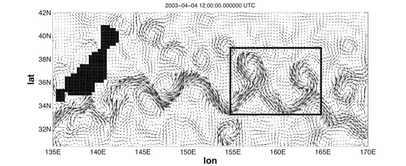
Figure 1: Velocity field of the Kuroshio current on April 4, 2003. The square highlights our main foucus area. Maximum values of the velocity field are about 3.65 m/s. (Figure taken from Mendoza et al. (2010)).

We focus over a region through which the Kuroshio Current passes, in April, May and June 2003. A typical velocity field is shown in Figure 1. Our transport description is mainly focused on the region highlighted with a rectangle. The equations of motion that describe the horizontal evolution of particle trajectories on a sphere are

$$\frac{d\phi}{dt} = \frac{u(\phi,\lambda,t)}{R{\rm cos}(\lambda)},$$ (4)

$$\frac{d\lambda}{dt} = \frac{v(\phi,\lambda,t)}{R}.$$ (5)

Here the variables ($\phi,\lambda$) are longitude and latitude; $u$ and $v$ respectively represent the eastward and northward components of the velocity field. The particle trajectories must be integrated in equations (4)-(5) and since information is provided solely in a discrete space-time grid, the first issue to deal with is that of interpolation. We have daily maps of the velocity field and this is a coarse time grid to provide a time step in the integration of particle trajectories, however this frequency sampling is adequate in the sense that changes of the vector field below that resolution are smooth enough to be approached by an interpolator. Days are a typical time scale for the system (4)-(5) and this is the unit of time in which results are reported. A recent paper by Mancho et al. (2006a) compares different interpolation techniques in tracking particle trajectories. Bicubic spatial interpolation in space (Press et al., 1992) and third order Lagrange polynomials in time are shown to provide a computationally efficient and accurate method. We use this technique in our calculations as it has been successfully implemented in realistic flows over a sphere as discussed in (Mancho et al., 2008). Following this work we notice that bicubic spatial interpolation requires a uniformly spaced grid, while our data grid is not uniformly spaced in the latitude coordinate. We transform our coordinate system to a new one ($\phi,\mu$), in which the latitude $\lambda$ is related to the new coordinate $\mu$ by

$$\mu={\rm ln}|{\rm sec}\lambda+{\rm tan}\lambda|$$ (6)

Our velocity field is now on a uniform grid in the ($\mu,\phi$) coordinates. The equations of motion in the new variables are,

$$\frac{d\phi}{dt} = \frac{u(\phi,\mu,t)}{R\,{\rm cos}(\lambda(\mu))}$$ (7)

$$\frac{d\mu}{dt} = \frac{v(\phi,\mu,t)}{R\,{\rm cos}(\lambda(\mu))}$$ (8)

In the numerical simulations the vector field in Eqs. (4)-(5) is represented in a selection of data spanning a domain in longitude and latitude $(\phi_{min},\phi_{max})\times(\lambda_{min},\lambda_{max})=(109.66^{o},259.66^{o})\times(14.74^{o},59.56^{o})$ which is much larger than those displayed in figures. This ensures that particle integrations do not cross the edges and thus boundary effects are not present. Variables $(\phi,\mu)$ are further transformed by scaling the domain to $(0,3)\times(0,1)$, which is more convenient for the manifolds computations reported in Section 4.2. The new variables are

$$x_{1}=3\frac{(\phi-\phi_{min})}{(\phi_{max}-\phi_{min})}$$ (9)

$$x_{2}=\frac{(\mu-\mu_{min})}{(\mu_{max}-\mu_{min})}$$ (10)

The scaling provides the dynamical system in which integrations are performed:

$$\frac{dx_{1}}{dt} = v_{1}(x_{1},x_{2},t)$$ (11)

$$\frac{dx_{2}}{dt} = v_{2}(x_{1},x_{2},t).$$ (12)

Once trajectories are integrated for presentation purposes, one can convert coordinates back to the original ones. In the reversion $x_{2}\to\mu\to\lambda$ we use the expression $\lambda(\mu)$ obtained by inverting Eq. (6), i.e.

$$\lambda=\frac{\pi}{2}-2\,{\rm arctan}(e^{-\mu})\ .$$ (13)

3 A time-depedent phase portrait

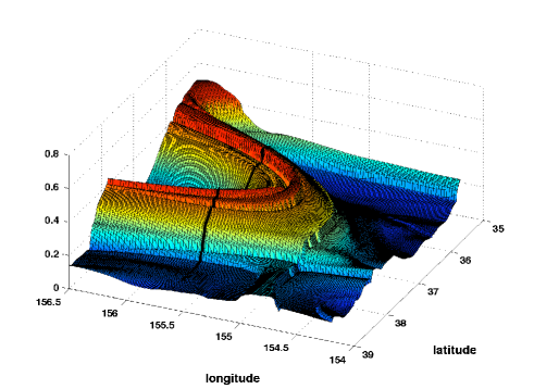
a)b)

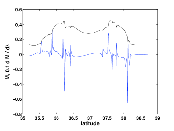
Figure 2: a) A representation of the function $M$ over a small oceanic area on May 2, 2003 for $\tau=15$ days; b) In black the function $M$ vs latitude at a fixed longitude highlighted in a) with the thick black line. Abrupt changes in $M$ pointing manifolds positions corresponds with discontinuities on the derivative. In blue 0.1 times the derivative of $M$ with respect the latitude.

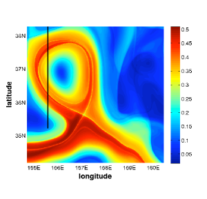
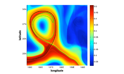
a)b)c)

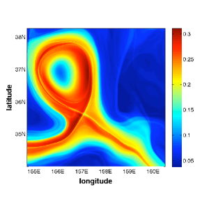
Figure 3: a) Contour plot of the function $M$ over a small oceanic area on May 2, 2003 for $\tau=15$ days. The black straight line corresponds to the selection for outputs in Fig 2 a) ; b) the same with a piece of stable manifold (black line) and a piece of unstable manifold (green line) overlapping; c) the function $M$ for $\mathcal{F}({\bf x}(t))=||{\bf a}({\bf x}(t),t)||$ and $\tau=15$ days in the same area.

Solutions of dynamical systems are qualitatively described according to Poincaré’s idea of seeking geometrical structures on the phase portrait. These can be used to organise particles schematically by regions corresponding to qualitatively different types of trajectories. In time independent systems –those in which Eq. (1) does not depend explicitly on time– fixed points are essential for describing the solutions geometrically. Fixed points may be classified as hyperbolic or non-hyperbolic depending on their stability properties. Stable and unstable manifolds of hyperbolic fixed points act as separatrices that divide the phase portrait in regions in which particles have different dynamical fates. To achieve this geometrical representation in time dependent aperiodic dynamical systems is a challenge, because the concepts used in autonomous dynamical systems do no apply directly to these systems. In these cases, structures containing Lagrangian information on the time-evolution of fluid particles have typically been obtained by means of Lyapunov exponents. The concept of Lyapunov exponent is infinite time and it is used in finite-time data sets for its finite-time versions such as finite-size Lyapunov exponents (FSLE) (Aurell et al., 1997) and finite-time Lyapunov exponents (FTLE) (Haller, 2001; Nese, 1989).

Different Lagrangian tools that also succeed in finding time dependent partitions for finite time aperiodic geophysical flows are proposed in this section. These implements are called Lagrangian descriptors. Lagrangian descriptors provide a global dynamical picture of arbitrary time dependent flows by detecting simultaneously the organizing centers of the flow, hyperbolic trajectories and their stable and unstable manifolds and elliptic regions. This technique has been successfully applied by de la Cámara et al. (2012) to stratospheric re-analysis data produced by the interim European Centre for Medium-Range Weather Forecasts (ECMWF) and has allowed the detection of dynamical features not perceived by other methods. Originally Lagrangian descriptors were introduced by Mendoza & Mancho (2010), in the context of altimeter velocity data, who proposed a function to this end. This function is referred to as $M$ and was advanced in Madrid & Mancho (2009) as a building block of the definition of Distinguished trajectories. These trajectories, their organizing role and their computation from $M$ are discussed further in the next section. We now focus on the capacity of $M$ as a Lagrangian descriptor. The function $M$ measures the Euclidean arc-length of the curve outlined by a trajectory passing through ${\bf x^{*}}$ at time ${t^{*}}$ on the phase space. The trajectory is integrated from ${t^{*}}-\tau$ to ${t^{*}}+\tau$. This is mathematically expressed as follows: For all initial conditions ${\bf x^{*}}$ in an open set ${\mathcal{B}}\in\mathbb{R}^{n}$, at a given time ${t^{*}}$, the Lagrangian descriptor is a function $M({\bf x^{*}},t^{*})_{{\bf v},\tau}:({\mathcal{B}},t)\to\mathbb{R}$ given by:

$$M({\bf x^{*}},t^{*})_{{\bf v},\tau}=\int^{t^{*}+\tau}_{t^{*}-\tau}\!\!\!\sqrt{\sum_{i=1}^{n}\left(\frac{dx_{i}(t)}{dt}\right)^{2}}dt$$ (14)

Here $(x_{1}(t),x_{2}(t),...,x_{n}(t))$ are the components in $\mathbb{R}^{n}$ of a trajectory ${\bf x}(t)$. The function $M$ depends on $\tau$ and also on the vector field v. It is defined for dynamical systems in arbitrary dimension $n$, but for the chosen system (11)-(12), $n=2$. The question is why should $M$ succeed in realizing Poincaré’s idea, revealing the geometry of objects such as the stable and unstable manifolds of hyperbolic trajectories? Mendoza & Mancho (2010) report this observed fact, and although it is not formally proven, an heuristic argument on this evidence is given. $M$ measures the arc-length of trajectories on a time interval $(t^{*}-\tau,t^{*}+\tau)$. For a given $\tau$ there may be trajectories that start and evolve close to each other and this of course may change with $\tau$. Trajectories which stay close are expected to have similar arc-lengths. However for this $\tau$, at the boundaries of regions comprising trajectories with qualitatively different evolutions, arc-lengths will change abruptly, and these regions are exactly what the stable and unstable manifolds separate. We evaluate $M$ as defined in Eq. (14) over the oceanic velocity field and a first output is provided in Figure 2. The coordinates at which sharp changes on $M$ occur are related to points of discontinuity on the derivative along a direction which is non tangent to the manifold. These are disclosed in Figure 2b). A contour plot of the same area, portrayed in Figure 3a), links the positions for these abrupt variations to lines resembling singular features. Figure 3b) visually demonstrates that the coordinates at which singular lines of the function $M$ are placed coincide with the positions of the stable and unstable manifolds. The Lagrangian information provided by $M$, that is the position of the invariant manifolds, is not contained on the specific values taken by $M$ but on the positions at which these values change abruptly. However in the interest of completeness, figures show a color bar indicating the range of $M$. Units correspond to those in the rescaled system (11)-(12).

Eq. (14) finds arc-lengths integrating the modulus of the velocity ($||{\bf v}||$) along a trajectory. It is easily observed that the heuristic argument should in fact work for the accumulation of other positive intrinsic geometrical or physical property along trajectories on a time interval $(t^{*}-\tau,t^{*}+\tau)$. For instance could have been considered integrations of the modulus of acceleration ($||{\bf a}||$), the modulus of the time derivative of acceleration ($||d{\bf a}/dt||$), or positive scalars obtained from combinations of ${\bf v}$, ${\bf a}$ or $d{\bf a}/dt$ as far as these combinations are bounded. In this way trajectories evolving close to each other during this time interval would accumulate a similar value for $M$, and the accumulated value of the property would be expected to change sharply at the boundaries of regions comprising trajectories with qualitatively different evolutions. These abrupt changes would highlight the stable and unstable manifolds. Our general method for building up families of Lagrangian descriptors for general time dependent flows replaces Eq. (14) by

$$M({\bf x^{*}},t^{*})_{{\bf v},\tau}=\int^{t^{*}+\tau}_{t^{*}-\tau}\mathcal{F}({\bf x}(t))\,dt.$$ (15)

where $\mathcal{F}({\bf x}(t))$ denotes a bounded positive intrinsic physical or geometrical property of the trajectory ${\bf x}(t)$. In practice not all choices of $\mathcal{F}({\bf x}(t))$ are equivalent. Typically for analyzing velocities fields given as data sets, choices involving $||d{\bf a}/dt||$ may be less appropriate than those involving ${\bf v}$ or ${\bf a}$ because they require interpolators with a higher order of regularity than the latter magnitudes. Similarly a choice involving ${\bf a}$ requires an interpolator with a higher regularity than those involving only ${\bf v}$. In this section we report results for $\mathcal{F}=||{\bf v}||$ and $\mathcal{F}=||{\bf a}||$. Both choices are adequate for the type of interpolation used in the velocity field. Many other options on $\mathcal{F}$ are thoroughly discussed and compared in (Mancho & Mendoza, 2011). For comparison purposes Figure 3c) shows the output obtained when $M$ is evaluated as in Eq. (15) with the choice $\mathcal{F}({\bf x}(t))=||{\bf a}({\bf x}(t),t)||$. As anticipated, singular lines in the contour plot coincide with the position of invariant manifolds. Full details of the numerical evaluation of $M$ are given in the Appendix A.

The heuristic argument pointed out above, supports the ability of Lagrangian descriptors for highlighting manifolds, but it is not a rigorous argument. The power of Lagrangian descriptors however is sustained by a strong numerical evidence consistently shown in all the examined examples, which thus inspires the development of further theoretical results.

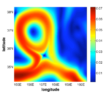
Figure 4: A representation of the function $M$ over a small oceanic area on May 2, 2003 for $\tau=2$ days. (Color version of a figure from Mendoza & Mancho (2010))

The function $M$ depends on $\tau$ in such a way that at low $\tau$, its structure is far from depicting manifolds. For instance, for $\tau=2$, Figure 4 shows a contour plot of $M$ for $\mathcal{F}({\bf x}(t))=||{\bf v}({\bf x}(t),t)||$, at the same coordinates as in Figure 3, but the observed structure is smooth and eulerian-like. The structure of $M$ at low $\tau$ is closely related to the spatial structure of the velocity field, thus for highly turbulent flows with a more complex spatial structure, $M$ is expected to display a richer pattern. Figure 5 shows contour plots of $M$ on April 17 over an area with an eddy-like vector field. For increasing $\tau$, $M$ displays more and more complex patterns and outlines a growing manifold structure.

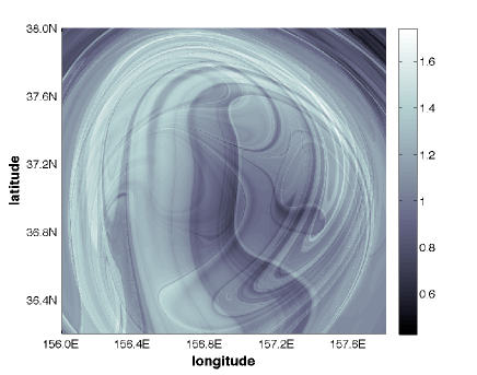
a)b)
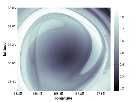
c)d)

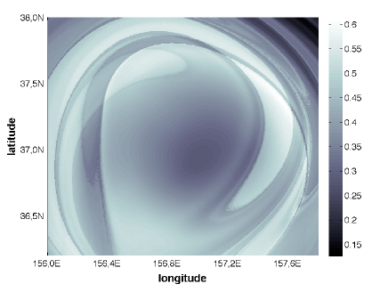
Figure 5: Lagrangian structure of the inner core of the western eddy on April 17 for increasing $\tau$ values. a) $\mathcal{F}({\bf x}(t))=|{\bf v}({\bf x}(t),t)|$ and $\tau=15$ days; b) $\mathcal{F}({\bf x}(t))=|{\bf v}({\bf x}(t),t)|$ and $\tau=30$ days; c) $\mathcal{F}({\bf x}(t))=|{\bf v}({\bf x}(t),t)|$ and $\tau=72$ days; d) $\mathcal{F}({\bf x}(t))=|{\bf a}({\bf x}(t),t)|$ and $\tau=30$ days.

In Figures 5a) and b), at low $\tau$ values the structure of $M$ at the inner part of the eddy has a minimum which is locally smooth. This implies that in the range $(t-\tau,t+\tau)$, trajectories in this vicinity outline similar paths: there are no sharp changes, and thus they behave as a coherent structure. The boundaries of this smooth region separate the mixing region (outside the core) from the non mixing region (inside). A comparison between Figures 5b) and 5d) confirms that both descriptors report similar outputs. In two-dimensional, incompressible, time-periodic velocity fields, this kind of structure is typical because the KAM tori enclose the core –a region of bounded fluid particle motions that do not mix with the surrounding region (Wiggins, 1992). However, there is no KAM theorem for velocity fields with a general time-dependence (Samelson & Wiggins, 2006) such as the one in our analysis. In this context, a question that remains open is to address the dispersion or confinement of particles in the core for aperiodic flows. In Figure 5c), for large $\tau=72$ days, the structure of $M$ in the interior of the eddy becomes less and less smooth, meaning that in the range $(t-\tau,t+\tau)$ trajectories placed at the interior core have either concentrated there from the past or will disperse in the future. In fact, the interior of the core is completely foliated by singular features associated either to stable or unstable manifolds of nearby hyperbolic trajectories. The non-smoothness of $M$ at $t={\rm April}\,\,17$ proposes $2\tau=144$ days as an upper limit for the time of residence of particles in the inner core; particles perceive nearby hyperbolic regions after this period. The accuracy of the singular lines of $M$ representing invariant manifolds is again confirmed in Figure 6, where computations of stable and unstable manifolds overlap those features. The foliated structure of $M$ is much richer than that provided by the displayed manifolds computed directly. This is so because the direct computation of manifolds requires the location of a priori special hyperbolic trajectories (also called DHTs as explained in next section) from which the manifold calculation starts. The selection of DHTs may leave out many other DHTs in the neighbourhood while $M$ exhibits all stable and unstable manifolds from all possible DHTs in the vicinity of the eddy, without the need for identifying them a priori. $M$ provides the complete visible foliation in the interval $(t-\tau,t+\tau)$ induced by the stable and unstable manifolds of all nearby hyperbolic trajectories.

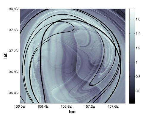
Figure 6: Stable and unstable manifolds overlapped on the function $M$ at day April 17 for $\tau=72$ days. There is a coincidence between singular features of $M$ and manifolds.

The evaluation of $M$ in large oceanic areas for long enough $\tau$, as shown in Figure 7, reveals recognisable phase portraits. The colour gradation of $M$ emphasises lasting and stronger features versus the ones that are weaker and more transient. Largest $M$ values are in red while the lowest are in blue. For instance in Figure 7a) the colours indicate that the strongest features are a central reddish stream and the one red and two yellow eddies. These are the most persistent patterns and because they remain for long periods of time it is possible to describe transport routes across them. Other recognisable bluish features such as the cat’s eyes at the upper left correspond to slow fluid motion. These features have a rapidly changing topology, and their lack of permanence makes it more difficult to describe transport across them, since transient structures are not well understood from the dynamical point of view (see Mancho et al. (2008); Branicki et al. (2011)). The function $M$ provides a global descriptor where different geometries of exchange are visualised in a straightforward manner. Figure 7b) shows the output of $M$ at the same area, at larger $\tau$ values. A more complex structure near the set of chaotic saddles is observed. The increasing of complexity of $M$ versus $\tau$ is expected from the nature of $M$, since it is reflecting the history of initial conditions on open sets, and in highly chaotic systems this history is expected to be more tangled for longer time intervals.

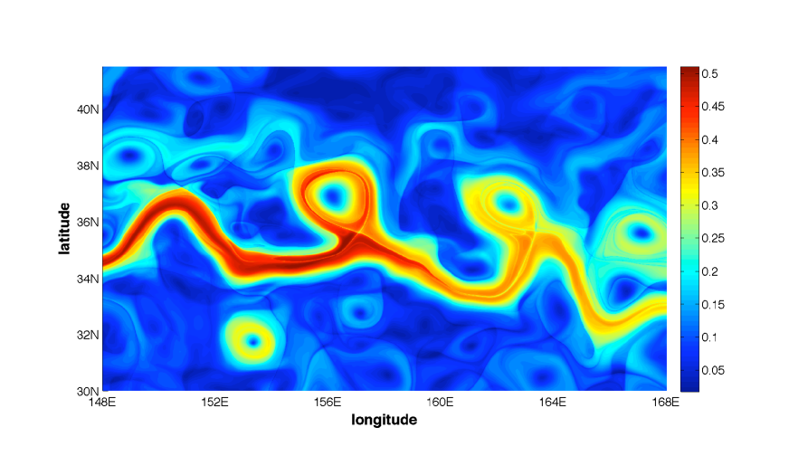
a) b)

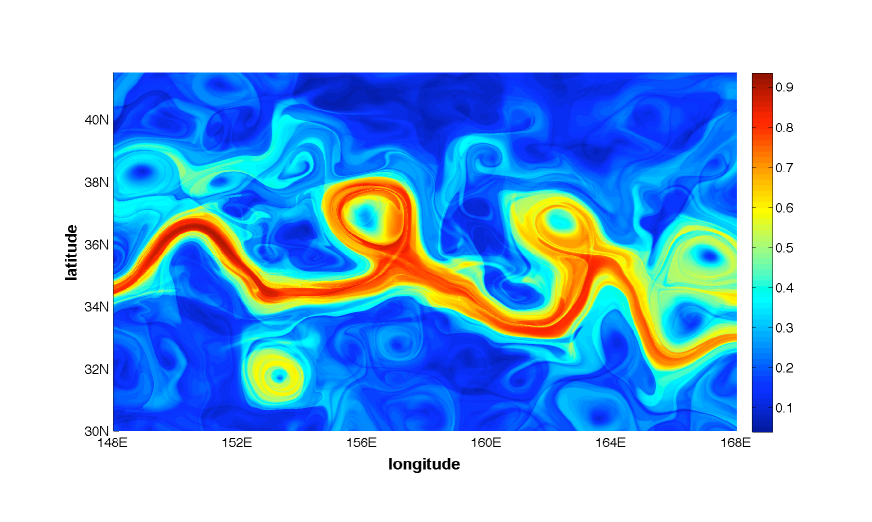
Figure 7: Evaluation of the function $M$ over the Kuroshio current between longitudes $148^{o}$E-$168^{o}$E and latitudes $30^{o}$N-$41.5^{o}$N on May 2, 2003; a) $\tau=15$ days; b) $\tau=30$ days. (Figure taken from Mendoza & Mancho (2010)).

Equation (15) proposes the integration along trajectories of a bounded positive intrinsic geometrical or physical property. Imposing the integration of a positive quantity is consistent with the perspective that Lagrangian descriptors reveal the dynamical structure by accumulating quantities along trajectories. When trajectories separate following different paths the accumulated quantity differs, and sharp changes on the descriptor values should occur at the boundaries of regions separating these qualitatively distinct behaviors, thereby highlighting the position of invariant manifolds. The accumulative perspective taken by Equation (15), although similar in its mathematical expression, is different from the finite-time average velocities used in Malhotra et al. (1998); Poje et al. (1999). In particular, these works consider the forward time integral of the velocity components divided by the time interval:

$$\frac{1}{\tau}\int^{t^{*}+\tau}_{t^{*}}\!\!\!v_{x}({\bf x},t)dt$$ (16)

This averaging is reported to reveal a patchiness structure which is also connected to invariant manifolds. In Poje et al. (1999), the authors note that for increasing averaging time a zero average velocity is obtained, and as a consequence in this limit the spatial structure in the patchiness plots is lost. As regards the integration time limits and their impact on the retrieved Lagrangian structure, the results by Poje et al. (1999) are the opposite of those obtained from the proposed Lagrangian descriptors. We have reported the existence of a minimum time $\tau$ to converge to the Lagrangian structures, which is not reported by Malhotra et al. (1998); Poje et al. (1999), and we have shown evidence that beyond that $\tau$, the longer $\tau$ is, the better and more detailed are the Lagrangian structures. The main reason for differences in the outputs between both methods is that the diagnosis by Poje et al. (1999) does not force the integral of a positive quantity, thereby allowing oscillations of the integrated quantity along trajectories, which produces non desired cancellations. Recently alternative methods which similarly to Lagrangian descriptors are based on measures along trajectories, have been described in Rypina et al. (2011). These methods have been successfully applied to describe Lagrangian Coherent Structures in geophysical flows.

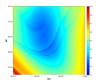
a)b)

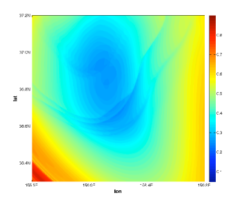
Figure 8: Contour plot of the function $M$ over the inner part of an eddy on May 2, 2003 for $\tau=30$ days a) results with bicubic spatial interpolation; b) results with bilinear spatial interpolation.

A question always under scrutiny is the robustness of the Lagrangian structures under errors. In the literature some results are found on this matter. For instance, Hernández-Carrasco et al. (2011) have studied the robustness of the Lagrangian structures under deviations induced in the vector field by noise and dynamics of unsolved scales. They have confirmed the permanence of the FSLE features under these perturbations. It is not our purpose to perform an analogue study on the function $M$. However Figure 8 presents some results in this regard. This figure estimates the reliability of $M$ by computing it with different interpolation schemes: bi-linear and bi-cubic spatial interpolation. The displayed results are structures obtained at large $\tau$ in the inner part of an eddy. The bi-linear spatial interpolation preserves the features obtained by the spatial bi-cubic interpolation, although it also adds some lines visible at the centre. Nevertheless the global appearance of the output is preserved.

The global dynamical picture provided by the function $M$ enables us to foresee active transport routes over the ocean surface. However, for describing detailed transport mechanisms associated to the recognisable phase portraits, the intricate curves making up manifolds must be accurately computed over the ocean surface. Extracting these curves from the above embroiled pictures is a difficult and imprecise task, doomed to failure, and for this reason we proceed in a different way, which is explained in the following section.

4 Distinguished trajectories and finite time invariant manifolds

The role of $M$ in transport description is based on its ability to cover the ocean surface with a geometrical structure that resembles a patchwork of interconnected dynamical systems, which indicates transport routes to be described in further detail. This important capacity cannot be achieved by the tools described in this section, which only provide details after the details themselves have been roughly identified a priori. Without this previous knowledge, the use of these tools is less effective because they are too focused and blind for distinguishing their own starting point. On the other hand the detailed transport routes reported by the tools described in this section cannot be obtained just by the use of Lagrangian descriptors. The scenario displayed by $M$ in Figure 7a) shows a strong jet, visible in the intense reddish band, and two eddies –interacting with the jet– which are visualised by two circles: one reddish situated towards the west side and the other yellowish to the east. For a detailed study of transport in this area we compute distinguished trajectories and manifolds.

4.1 Distinguished trajectories

The stable and unstable manifolds of special hyperbolic trajectories such as fixed points in autonomous dynamical systems or periodic trajectories in periodically time dependent systems are the ones of interest in our study. These trajectories, which act as organizing centres of the flow, do not have a natural extension for time-dependent aperiodic dynamical systems, in which a generalization of these concepts is required. The definition of distinguished hyperbolic trajectories (DHTs) has succeeded to this end. Several definitions have been proposed, for instance see Ide et al. (2002); Ju et al. (2003); Madrid & Mancho (2009). In this article we follow the approach to these trajectories reported by Madrid & Mancho (2009), which is based on the Lagrangian descriptor given by the function $M$ in Eq. (14).

The concept of DT generalizes the idea of fixed point for time-dependent dynamical systems. For instance for the 1D time-dependent linear system:

$$\frac{dx}{dt}=-x+t$$ (17)

the particular solution $x_{p}(t)=t-1$ is a generalized fixed point. It is considered so, because the equation (17) by means of the Galilean transformation:

$$x^{\prime}=x+vt$$ (18)

is converted into the autonomous system:

$$\frac{dx^{\prime}}{dt}=-x^{\prime}-1$$ (19)

which has a fixed point at $x^{\prime}_{p}=-1$. The Galilean transformation (18) applied to this fixed point transforms it back into the particular solution $x_{p}(t)=t-1$. The intuitive geometrical idea behind our definition for identifying $x_{p}$ as distinguished is to search for a trajectory that ”moves less” than others in a vicinity. But what does this mean?. For a given initial condition ${\bf x^{*}}$ on an open set ${\mathcal{B}}$ at a given time $t^{*}$, “move less” is satisfied by a trajectory that minimizes $M$ in Eq. (14). This function measures the arc-length of the curve outlined on the phase space by the trajectory passing through $({\bf x}^{*},t^{*})$ from $t^{*}-\tau$ to $t^{*}+\tau$. In Figure 9a), $M$ is represented for the system (17) at $t=0$ for $\tau=3,4$. It is observed that $M$ reaches a minimum at different positions ${\bf x}^{*}$ for different $\tau$. However although this fact may involve ambiguity in locating the position for a DT, at large $\tau$ the position of the minimum converges towards what is called the limit coordinate. Figure 9b) confirms this point. There the position ${\bf x}^{*m}$ at which $M$ reaches its minimum is plotted, which for increasing $\tau$ approaches the value $x=-1$. This is exactly the passing point of the particular solution $x_{p}$ at $t=0$. In practice as noted by Madrid & Mancho (2009) the convergence to the limit coordinates cannot be examined in the limit $\tau\to\infty$ either because it is impracticable in a numerical implementation, or because in the large limit errors accumulate, or simply because the dynamical system is defined by a finite time data set. For these reasons the convergence to the limit coordinates is tested up to a finite $\tau$. Formally this is expressed as follows: Let us consider a practicable time interval $[T_{i},T_{f}]$, let be ${\bf x}^{m*}_{t_{l}}(\tau)$ the coordinates at which the function $M$ reaches the minimum value at time $t_{l}$ in an open set ${\mathcal{B}}$. Then to find the limit coordinate ${\bf x}^{l}$ at time $t_{l}$ we verify that there exists a $\tau^{l}$ such that: $t_{l}-\tau^{l}>>T_{i}$, $t_{l}+\tau^{l}<<T_{f}$ and $\forall\tau>\tau^{l}$ the following is satisfied: $||{\bf x}^{m*}_{t_{l}}(\tau)-{\bf x}^{l}(t_{l})||\leq\delta$ (where $\tau$ keeps $t^{l}-\tau>T_{i}$ and $t_{l}+\tau<T_{f}$ and $\delta$ is a small positive constant). Here $||\cdot||$ represents the distance defined by

$$||{\bf a}-{\bf b}||=\sqrt{\sum_{i=1}^{n}(a_{i}-b_{i})^{2}}\,\,\,\,\,{with}\,\,\,\,{\bf a},{\bf b}\in\mathbb{R}^{n}.$$

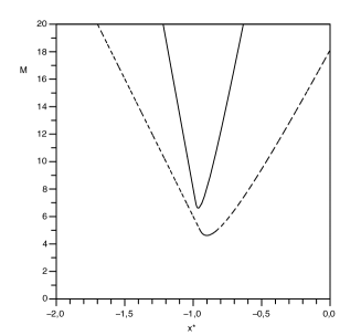
a)b)

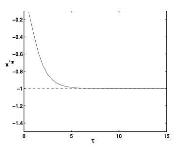
Figure 9: a) The function $M$ at $t=0$ for $\tau=3$ (dashed line) $\tau=4$ (solid line); b) evolution of the coordinate ${\bf x}^{*m}$ at which $M$ reaches a minimum versus $\tau$ at $t=0$. (Figure taken from Madrid & Mancho (2009)).

By repeating the procedure at different times $t$, it is possible to obtain a path of limit coordinates which is denoted as ${\bf x}^{l}(t)$. The distinguished trajectory $\gamma(t)$ is thus defined in a time interval $[t_{0},t_{N}]$ as that trajectory that is close enough (at a distance $\epsilon$) to a path of limit coordinates. According to (Madrid & Mancho, 2009) this is expressed formally as follows: A trajectory $\gamma(t)$ is said to be Distinguished with accuracy $\epsilon$ ($\,0\leq\epsilon$ ) in a time interval $[t_{0},t_{N}]$ if there exists a continuous path of limit coordinates $(t^{l},{\bf x}^{l})$ where $t^{l}\in[t_{0},t_{N}]$, such that,

$$||\gamma(t^{l})-{\bf x}^{l}(t^{l})||\leq\epsilon,\,\,\forall t^{l}\in[t_{0},t_{N}]$$ (20)

In this definition $\epsilon$ is a small positive constant within the numerical accuracy we can reach. Further examples of trajectories characterized as Distinguished are discussed in the work by Madrid & Mancho (2009) in two and three dimensions.

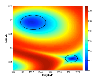
a)b)

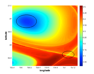
Figure 10: Contour plots of the function $M$ on May 2, 2003 in the nearby of two positions which are candidates to be DT. a) $\tau=2$ days; b) $\tau=15$ days.

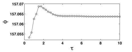
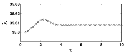
Figure 11: Evolution of the longitude and latitude position of the hyperbolic minimum of the function $M$ on May 2, 2003 versus $\tau$ (in days).

Next we illustrate how to identify DT in our 2D data set. Figure 10a) shows a contour plot of $M$ on $t^{*}=$May 2, 2003 for $\tau=2$ days in the neighbourhood of the western eddy. Two circles surround the two minima of this open set. These minima correspond to initial conditions whose trajectories outline curves shorter on the phase space than those in their vicinity. Figure 10b) shows the same contour plot of $M$, but at $\tau=15$ days. A comparison with figure 10a) reveals several differences. The neighbourhood of the minimum in the lower circle of Fig 10b) presents a crossed-line structure, that has been linked to manifolds. In the interior of this structure there exists a minimum whose position does not coincide with that obtained at $\tau=2$ days. Figure 11 shows the evolution of the longitude and latitude position of the minimum with $\tau$ converging to a limit coordinate. In figure 10b), the minimum in the lower circle has reached the position of the limit coordinate within the accuracy $\epsilon$ available with our numerical schemes. It is possible to track in a set of discrete times $t^{l}$ the path $(t^{l},{\bf x}^{l})$ described by this limit coordinate in a time interval. The path is displayed in Figure 12. In the vicinity of the path displayed in Fig 12 at a distance $\epsilon$ is found DHT_W, a trajectory that remains distinguished from March 5 to May 11, 2003. Figure 12 also represents the coordinates of a second trajectory labelled as DHT${}^{+}_{W}$, in an almost complementary period of time, between May 10 and June 1, 2003. Trajectories DHT_W and DHT${}^{+}_{W}$ were first characterised in this data set by Mendoza et al. (2010). By construction, a Distinguished Trajectory defined in this way is a property held by some trajectories in finite time intervals. Alternative definitions such as those provided in Ide et al. (2002); Ju et al. (2003) do not address this possibility.

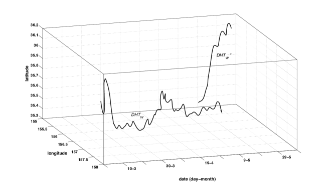
Figure 12: Path of limit coordinates for DHT_W and DHT${}^{+}_{W}$.

The ideas described above are itemised in the algorithm that computes DT, and is fully described in Madrid & Mancho (2009). We give a brief account of it next. It starts by estimating an approximate position ${\bf x}^{*m}$ for the minimum of $M$ at low $\tau$ in a specific area at a given time $t^{*}$. Its coordinates are refined up to a precision $\delta$ by considering a grid such as that depicted in Figure 13, which has its centre positioned at ${\bf x}^{*m}$. $M$ is evaluated in the nodes of the grid and if the lowest $M$-value is not taken at the centre, but in a peripheral node the grid displaces its centre at this position of the minimum, which provides a better approach for ${\bf x}^{*m}$. $M$ is then reevaluated in the nodes of the new positioned grid, and if the minimum is found to be at the central node, the search stops. This method is used to follow the position of the minimum at iteratively increasing $\tau$: $\tau_{k}=\tau_{k-1}+\Delta\tau$, where $\Delta\tau$ is a small quantity. The procedure stops when the position of the minimum ${\bf x}^{*m}$ does not change for further $\tau$ increments. At the next time $t^{*}+\Delta t$, ${\bf x}^{*m}$ is time evolved with the equations of motion, and the iterative search described above starts from this point.

Figure 13: The grid used to find the minimum position with precision $\delta$. The white central dot indicates the position where the minimum is due.

The minimum situated in the interior of the upper circles in Figure 10 presents a structure that evolves with $\tau$ quite differently to what is found in the lower circles. It remains rather flat and circular and does not evolve towards the crossed line structure typical of DT with hyperbolic stability (DHT). As discussed in (Madrid & Mancho, 2009) these patterns are typical of a DT with elliptic stability (DET). Figure 14 shows the evolution of the coordinates of this minimum versus $\tau$. In this case, a DET is not properly identified, because contrary to what is found for hyperbolic cases, a limit coordinate is not reached. DETs are not easily found in highly aperiodic flows. A previous attempt has been discussed in Madrid & Mancho (2009) for a different data set, and a failure to satisfy the definition is reported. Successful examples of DET are however reported for time periodic dynamical systems (see Madrid & Mancho (2009) for full details).

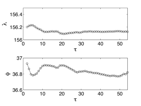
Figure 14: Evolution of the longitude and latitude position of the elliptic minimum of the function $M$ on May 2, 2003 versus $\tau$ (in days).

Although this elliptic minimum is not related to a special trajectory, it still locates a coherent structure related to an oceanic eddy. As reported in the previous section, particle confinement on this area persists in a time interval $[t^{*}-\tau,t^{*}+\tau]$ provided that $\tau$ is below the limit at which the foliation induced by the stable and unstable manifolds of nearby hyperbolic trajectories penetrates the inner core. Precisely the fact that these eddy-like structures eventually perceive nearby hyperbolic trajectories, would justify the absence of DETs in their interior.

In the scenario shown in by Figure 7a), at the east bound the jet interacts with the yellowish eddy to form a crossed line structure which is identified as an eastern DHT. The path of limit coordinates near this DHT_E is represented in Figure 15. It stays as distinguished between March 25 and June 24, 2003 (see also Mendoza et al. (2010)).

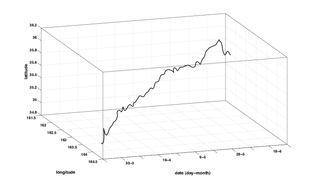
Figure 15: Path of limit coordinates for DHT_E.

4.2 Finite time invariant manifolds

Invariant manifolds are mathematical objects classically defined for infinite time intervals. The unstable (stable) manifold of a hyperbolic fixed point or periodic trajectory is formed by the set of trajectories that in minus (plus) infinity time approach these special trajectories. In geophysical contexts this definition is not realizable, because on the one hand only finite time aperiodic data sets are possible and on the other hand the reference trajectories, the DHTs, typically hold the distinguished property in finite time intervals. However, a detailed description of Lagrangian transport requires a direct computation of the stable and unstable manifolds of the selected DHTs. Branicki & Wiggins (2009) have recently proposed a novel algorithm to compute invariant manifolds in 3D non-autonomous dynamical systems. Nevertheless our next presentation is focused on the illustration of this procedure in 2D flows as corresponds to the selected data set. Mancho et al. (2004, 2008); Mendoza et al. (2010); Branicki et al. (2011) have computed stable and unstable manifolds of DHTs for 2D highly aperiodic data sets by using the method proposed in (Mancho et al., 2003). Based on ideas and techniques of contour advection (Dritschel, 1989; Dritschel & Ambaum, 1997), the algorithm computes manifolds as curves advected by the velocity field, which at the beginning of the procedure are small segments aligned with the stable and unstable subspaces of the DHT. The use of these small segments in the starting step is the way to build a finite-time version of the asymptotic property of manifolds. Hence in our computations the finite-time unstable manifold at a time $t^{*}$ is made of trajectories that at time $t_{0}$, $t_{0}<t^{*}$ were at a small segment aligned with the unstable subspace of the DHT. Similarly the finite-time stable manifold at a time $t^{*}$ is made of trajectories that at a time $t_{N}$, $t_{N}>t^{*}$ are in a small segment aligned with the stable subspace of the DHT. Localising thus a DHT and its stable and unstable directions at the starting time constitutes the first step. The way in which the stable and unstable subspaces are identified is closely related to the way in which DHTs are computed. For instance algorithms for DHTs described in Ide et al. (2002); Ju et al. (2003) provide them directly as an output, and this is the start-up for the manifolds computed in Mancho et al. (2004, 2008); Branicki et al. (2011). The algorithm for DHTs reported in Madrid & Mancho (2009), which is the one followed in this work, does not provide these subspaces, but we note that stable and unstable subspaces are supplied by the crossed lines recognised in the contour plots of the function $M$ near the DHT. These lines, as reported in Mendoza & Mancho (2010); Mendoza et al. (2010), are advected by the flow and constitute a close-up of the manifold near the DHT. Segments within the stable and unstable subspaces of the DHT are respectively evolved backward and forward in time to obtain the fully nonlinear stable and unstable manifolds (Mendoza et al., 2010). We focus on describing the details for obtaining the unstable manifold, noting that the stable manifold is obtained in a completely analogous way by inverting the time direction. The unstable manifold is represented at time $t_{0}$ by a set of points on the unstable subspace. The manifold is computed in a discrete set of time increments $t_{k}$ for $k=0...N$, in which it is represented by a well chosen set of points. We explain how to determine these points at every time $t_{k}$. The procedure starts by considering the points on the initial segment which are evolved in time from $t_{0}$ to $t_{1}$. As they evolve they may grow apart, giving rise to unacceptable large gaps between adjacent points on the manifold. The criterion for unacceptable gaps is given by a quantity $\sigma_{j}$ which is defined at each point ${\bf x}_{j}$ as the product of the distance $d_{j}$ between adjacent nodes ${\bf x}_{j}$ and ${\bf x}_{j+1}$ times the density $\rho_{j}$, i.e, $\sigma_{j}=d_{j}\rho_{j}$. If $\sigma_{j}>1$ the gap between nodes is unacceptable. The density of points along the computed manifold is measured by $\rho_{j}$, for which several expressions are proposed (Dritschel, 1989; Dritschel & Ambaum, 1997). We consider it defined as in Eq. (51) in the Appendix B. When a gap between nodes at time $t_{1}$ is too large according to the criterion just defined, it is filled by inserting a point at $t_{0}$ between the same nodes using an appropriate interpolation technique. At this stage the interpolation could be simple because the curve at $t_{0}$ is a straight line. However most refined interpolation techniques are required when this procedure is applied to evolve the manifold from $t_{k}$ to $t_{k+1}$ for $k>0$, since manifold becomes more and more intricate. The most successful interpolation scheme of those used in Mancho et al. (2003, 2006b) is due to Dritschel (1989). This method represents the curve between points ${\mathbf{x}}_{j}$ and ${\mathbf{x}}_{j+1}$ as the polynomial given by Eq. (57) in the Appendix B. The criterion is verified for each pair of adjacent points making up the manifold at $t_{1}$ and the procedure is iterated until there are no gaps exceeding the tolerance. Once the gap size acceptability condition is satisfied at $t_{1}$ we use the point redistribution algorithm described in (Dritschel, 1989) in an attempt to remove points from less computationally demanding parts of the manifold (see Mancho et al. (2004)). This algorithm works as we describe in the Appendix B. The complete procedure to evolve the unstable manifold from $t_{0}$ to $t_{1}$ is repeated for successive times $t_{k-1}$, $t_{k}$ until the end time $t_{N}$ is reached. Stable manifolds are obtained in a similar way, but the computation is started at time $t_{N}$.

Examples of manifolds computed with this method are shown in Figures 6 and 16 for the western DHT_W. Manifolds computed in this way become very long and intricate curves and from them transport is described in great detail as discussed in the next section.

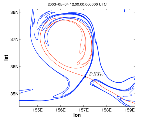
Figure 16: Stable (blue) and unstable (red) manifolds of DHT_W on the 4th of May 2003. (Figure taken from Mendoza et al. (2010)).

Almost every distinguishable line in Figure 16 contains numerous foldings of each manifold, thus confirming how intricate they may be. Other approaches such as FTLE or FSLE compute manifolds at a given time as ridges of a scalar field, thereby providing pieces of curves that are approximately material curves. However, in these approaches links between pieces of curves are difficult to establish as they fade away and this is a disadvantage compared with the direct computation of manifolds, which provides long complex linked curves due to the asymptotic condition imposed in their computation.

As noted in the previous subsection, DHT_W is characterized as Distinguished in a finite-time interval: from March 5, to May 11 2003. A question then to be addressed is, what happens to the unstable manifold in Figure 16 beyond May 11, once DHT_W losses its distinguishing property? It is observed that the manifold computation beyond this time may continue, because even if the reference trajectory on it is lost, the computation still provides a material surface advected by the flow, and second this advected object is still asymptotic to DHT_W in the finite-time sense introduced above. A similar argument can be made for the stable manifold in times prior to March 5. DHTs and their stable and unstable subspaces are the starting step of the algorithm for direct computation of manifolds. However, as reported in Mancho et al. (2004, 2006b) they are not required by the algorithm beyond this point. Nevertheless it is useful to have the full track of the DHT for transport description purposes, because it marks a reference point which separates the manifold into two branches. Section 5 illustrates the application of this division.

4.3 Frame invariance

In this section we discuss the issue of ‘frame invariance”. To begin with, it is important to understand what is meant by this phrase in the context of our work. There are two main issues. One is how the Lagrangian tools, such as those based on $M$, perform in different coordinate systems. The other is how stability and geometrical features of the flow transform under coordinate transformations. It is expected that under coordinate transformations the results obtained from the $M$ function will transform according to the manner in which the type of invariant objects that the $M$ function is expected to recover transform. However, we note that in general these invariant objects are not preserved under arbitrary coordinate transformations, as we will illustrate in this section. Three examples will provide evidence of these issues below.

The function $M$ is used for two different purposes. One is discovering and visualising the global dynamics of a time-dependent velocity field $M$ realises manifolds at positions at which abrupt changes in $M$ occur. If the coordinates of a dynamical system are transformed to a rotating frame or to a frame moving with a constant velocity (i.e. a Galilean transformation of the coordinates) the manifolds will transform to manifolds in the new coordinate system under the same transformation of coordinates. Of course the values of $M$ at specific points of space will certainly change with the reference frame, but the edges at which $M$ changes abruptly – which are the features containing the Lagrangian information– are transformed with the change of coordinates in the same manner in which the manifolds themselves are transformed. This is expected to be the case since the heuristic argument introduced to justify why $M$ detects manifolds is independent of a particular coordinate frame–manifolds play the role of dividing the phase space into regions corresponding to particles with qualitatively different dynamical fates and this is the case for any reference frame.

We verify this argument for the periodically forced Duffing equation under the rotation:

$$R(t)=\left(\begin{array}[]{cc}\cos\omega t&-\sin\omega t\\ \sin\omega t&\cos\omega t\end{array}\right).$$ (23)

In the rotating frame this equation takes the form:

$$\left(\begin{array}[]{c}\dot{\eta_{1}}\\ \dot{\eta_{2}}\end{array}\right) = \left(\begin{array}[]{cc}\sin 2\omega t&\cos 2\omega t+\omega\\ \cos 2\omega t-\omega&-\sin 2\omega t\end{array}\right)\left(\begin{array}[]{c}\eta_{1}\\ \eta_{2}\end{array}\right)$$ (30)

$$+ (\varepsilon\sin t-[\cos\omega t\eta_{1}-\sin\omega t\eta_{2}]^{3})\left(\begin{array}[]{c}\sin\omega t\\ \cos\omega t\end{array}\right).$$ (33)

The Duffing equation in the non-rotating system:

$$\dot{x_{1}} = x_{2}$$ (34)

$$\dot{x_{2}} = x_{1}-x_{1}^{3}+\epsilon\sin(t)$$ (35)

possesses a distinguished hyperbolic trajectory (DHT). This DHT can be computed as a perturbation expansion in $\epsilon$ about the hyperbolic fixed point in the $\epsilon=0$ case:

$${\bf x}_{DHT}(t)=-\frac{\varepsilon}{2}\binom{\sin t}{\cos t}-\frac{\varepsilon^{3}}{40}\binom{2\sin^{3}t+\frac{3}{2}\sin t\cos^{2}t}{\frac{3}{2}\cos^{3}t+3\sin^{2}t\cos t}+\mathcal{O}(\varepsilon^{5}).$$ (36)

The DHT in the rotating frame ${\boldsymbol{\eta}}_{DHT}$ is obtained by transforming the DHT in the non-rotating frame with the coordinate transformation:

$${\boldsymbol{\eta}}_{DHT}(t)=R(t)^{-1}{\bf x}_{DHT}(t).$$ (37)

Stable and unstable manifolds of ${\boldsymbol{\eta}}_{DHT}$ are computed for $\omega=2$ and $t=1$ thereby obtaining the output displayed in Figure 17a). These manifolds have been obtained with the algorithm reported in Subsection 4.2 which follows the approach by Mancho et al. (2003, 2004). The figure confirms that manifolds are objects rotating with the coordinates. Figure 17b) confirms that the Lagrangian descriptors discussed in Section 3 provide the same manifolds in the rotated frame.

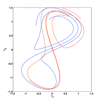
a)b)

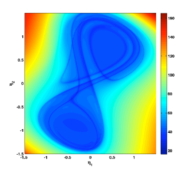
Figure 17: a) Invariant manifolds for the rotating Duffing equation for $\omega=2$ and $t=1$; b) contour plot of descriptor $M$ for $\mathcal{F}=|{\bf v}|$ with $\tau=10$ at the same $\omega$ and $t$ values.

A second use of the function $M$ is the computation limit coordinates that are at the basis of the definition of distinguished trajectory given in Madrid & Mancho (2009). In this paper the authors have shown that the definition of DT discussed in 4.1 is robust with respect to rotations in the sense that in the rotating frame the expression ${\boldsymbol{\eta}}_{DHT}$ is equally characterized as Distinguished.

The linear example in section 4.1 also illustrates that translations with constant velocity preserve Distinguished Trajectories (DT) in the sense that in the new frame of reference the transformed DT also preserves the property of being Distinguished. However not all coordinate transformations preserve Distinguished Trajectories. In particular, coordinate transformations involving trajectories of the velocity field do not necessarily preserve fixed points or their stable and unstable manifolds, and we illustrate this next.

Let us consider the dynamical system:

$$\frac{dx}{dt} = x-1$$

$$\frac{dy}{dt} = -y$$ (38)

for which $(x=1,y=0)$ is a hyperbolic fixed point. Let us consider the trajectory ${\bf x}^{p}(t)$:

$${\bf x}^{p}(t)=\binom{1.5{\rm e}^{t}+1}{0.5{\rm e}^{-t}}.$$ (39)

A coordinate transformation based on this trajectory is the following:

$${\bf x}^{N}={\bf x}-{\bf x}^{p}(t),$$ (40)

which transforms the system (38) into:

$$\frac{dx^{N}}{dt} = x^{N},$$

$$\frac{dy^{N}}{dt} = -y^{N}.$$ (41)

This is again an autonomous dynamical system with a hyperbolic fixed point at $(x^{N}=0,y^{N}=0)$. The time dependent coordinate transformation (40) obviously does not transform this fixed point into the old one $(x=1,y=0)$. Moreover this transformation does not preserve the stable and unstable manifolds themselves. The unstable manifold of the fixed point $(x,y)=(1,0)$ in the original system is given by:

$${\bf x}_{u}=\binom{\alpha+1}{0}$$ (42)

for arbitrary real $\alpha\neq 0$. On the other hand the unstable manifold of the hyperbolic fixed point $(x,y)=(0,0)$ in the transformed system is given by:

$${\bf x}^{N}_{u}=\binom{\beta}{0}$$ (43)

for arbitrary real $\beta\neq 0$. The transformation (40) does not map a point in the unstable subspace ${\bf x}_{u}$ to a point in the unstable subspace ${\bf x}^{N}_{u}$ since in general:

$$\binom{\beta}{0}\neq\binom{\alpha+1}{0}-\binom{1.5{\rm e}^{t}+1}{0.5{\rm e}^{-t}}.$$ (44)

We note that time-dependent transformations based on trajectories may have even more dramatic effects on invariant objects, such as tori. For example, if ${\bf x}^{p}(t)$ corresponds to a trajectory in a torus in the original system it will transform to a fixed point under this transformation.

Finally, we consider another example of a transformation of coordinates based on trajectories of the original system. Consider the one-dimensional autonomous system:

$$\frac{dx}{dt}=c$$ (45)

where $c$ is a nonzero constant constant. This system has no fixed points However if we consider the transformation (40) based on any trajectory of (45) ${\bf x}^{p}(t)=ct+d$:

$${\bf x}^{N}={\bf x}-(ct+d),$$ (46)

the system becomes:

$$\frac{dx^{N}}{dt}=0$$ (47)

which is also autonomous and all initial conditions are fixed points. We note that the reason that the transformation (46) does not preserve fixed points is that it is based on a trajectory of the original system, despite the fact that it is a Galilean transformation.

Finally, we remark that it has been often stated that Lagrangian “structures” and analytical methods should be frame-independent (see for instance Farazmand & Haller (2012)). However, from these examples we see that fixed points and invariant manifolds of hyperbolic fixed points may not be preserved by transformations based on particle trajectories. This indicates that more reflection is required on what is meant in this context by frame-independence and what truly must be demanded of geometrical structures and analytical tools for useful Lagrangian descriptions.

5 Transport routes across the ocean surface

In this section we show how to obtain transport information from the output of the tools described in previous sections. We start by describing transport across eddies displayed in Figure 7. Particles in their interior, despite belonging to flows in a quite chaotic regime, as is the case of the ocean surface, typically do not experience the butterfly effect which is characterised by a high sensitivity to initial conditions. On the contrary, particles contained therein remain gathered together for long periods of time, during which they form spatially coherent structures. Mathematically, eddies are related to non-hyperbolic flow regions, where particles evolve mostly “circling”. The exponentially increasing separation between particles is characteristic of hyperbolic regions, which are also responsible for unpredictability. Essentially transport across the ocean surface is governed by the interplay between these dispersive and non dispersive objects. The Lagrangian description of eddies identifies the existence of an outer collar, where the interchange with the media is understood in terms of lobe dynamics (see Joseph & Legras (2002); Branicki et al. (2011)) and an inner core, which is robust and rather impermeable to stirring, as already described in section 3. In this section we focus on describing transport across the outer part of the eddy which is located at the west end in Figure 7. The stable and unstable manifolds of $DHT_{W}$, which are involved in the transport across this vortex, are shown in Figure 16. These manifolds confirm the exchange of water by the presence of the turnstile mechanism for a period of one month from March 19 to April 23. The turnstile mechanism has been extensively used and explained in the literature (Malhotra & Wiggins, 1998; Rom-Kedar et al., 1990), and has been found to play a role in transport in several oceanographic contexts (Mendoza et al., 2010; Mancho et al., 2008; Coulliette & Wiggins, 2001). This mechanism is described from pieces of stable and unstable manifolds of the identified DHT. A first point to address is the selection of those pieces of invariant manifolds from messy curves such as those in Figure 16. For this purpose we consider that a manifold has two branches separated by the DHT which is taken as a reference point on the manifold, and selections of portions of manifolds are made from this reference point. Given that trajectories may retain the distinguished property only in finite time intervals, the identification of the two branches on the manifold is possible only on time intervals when the trajectory remains distinguished. Beyond that time the manifold computation may continue, but the reference point on it is lost. The turnstile mechanism identifies masses of water crossing a time-dependent Lagrangian barrier separating the inside from the outside. The Lagrangian barrier around the vortex in Fig 16 at a time $t_{k}$ is defined by selecting a branch of the unstable manifold which starts at DHT_W and surrounds the eddy towards the left side and a branch of the stable manifold which starts at DHT_W and surrounds the eddy towards the right side. We choose the segments considering that they must intersect at precisely one point $a_{t_{k}}$ and that they must form a relatively smooth boundary (i.e, free of the violent oscillations displayed by each of the manifolds when approaching DHT_W from the opposite side). Figure 18 shows the selections outlining the barriers for the dates $t_{1}=$March 19 and $t_{2}=$April 3, 2003. The blue line stands for the stable manifold while the red line corresponds to the unstable manifold. The boundary intersection points are marked as $a_{t_{1}}$ and $a_{t_{2}}$. Intersection points are invariant, which means that if the stable and unstable manifolds intersect in a point at a given time, then they intersect for all time, and the intersection point is hence a trajectory. For a better understanding of the time evolution of lobes, the positions of trajectories $a_{t_{1}}$ and $a_{t_{2}}$ are depicted at different times. Figure 19 shows longer pieces of the unstable and stable manifolds at the same days as those selected in Figure 18. Manifolds intersect forming regions called lobes. Only the fluid that is inside the lobes can participate in the turnstile mechanism. Two snapshots showing the evolution of lobes from March 19 to April 3 are displayed. There one may observe how the lobe which is inside the eddy on March 19 goes outside on April 3. Similarly the lobe which is outside on March 19 is inside on April 3. Trajectories $a_{t_{1}}$ and $a_{t_{2}}$ are depicted, showing that they evolve, circulating clockwise around the DHT_W. The green colour applies to the lobe that evolves towards the interior of the eddy while the magenta area evolves from the inside towards the outside. Between March 19 and April 23, several lobes are formed, mixing waters at both sides of the eddy. Figure 20 contains a time sequence showing the evolution of several lobes created by the intersection of the stable and unstable manifolds. The selected days are: $t_{2}=$April 3, $t_{3}=$April 10, $t_{4}=$ April 17 and $t_{5}=$ April 23. A sequence of trajectories $a_{t_{1}},a_{t_{2}},a_{t_{3}},...$ obtained from the intersection points is depicted. These trajectories evolve clockwise, surrounding the vortex, and serve as references for tracking lobe evolution. Beyond April 23 we cannot locate further intersections between the stable and unstable manifolds of DHT_W. Hence, no more lobes are found, and our description of the turnstile mechanism ceases.

a)b)

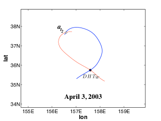
Figure 18: Lagrangian barriers for the western eddy at dates March 19 and April 3, 2003. These have been made from finite length pieces of the stable and unstable manifolds of DHT_W. The boundary intersection points are denoted respectively by $a_{t_{1}}$ and $a_{t_{2}}$.

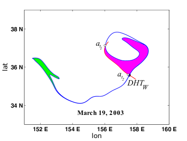
a)b)

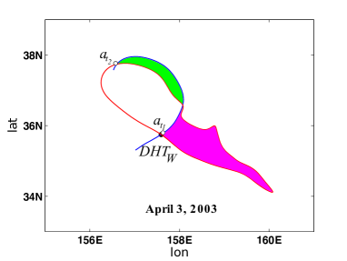
Figure 19: Turnstile lobes across the western eddy at dates March 19 and April 3, 2003. The intersection trajectories $a_{t_{1}}$ and $a_{t_{2}}$ are displayed at both dates showing their clockwise circulation around the eddy. The magenta area evolves from the inside to the outside while the green area does from the outside to the inside.

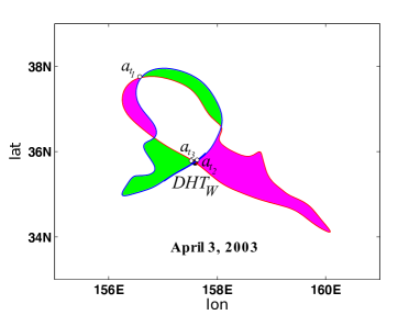
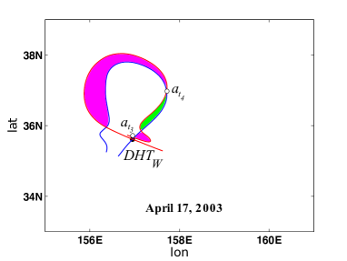
a)b)
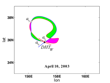
c)d)

Figure 20: Sequence of lobes mixing waters from inside the eddy to outside and viceversa in selected days of year 2003. a) April 3; b) April 10; c) April 17; d) April 23.

The turnstile mechanism across the eddy coexists in time with other transport routes observed, for instance, across structures such as the reddish main current in Figure 7. Mendoza et al. (2010) have addressed transport across this jet in terms of DHT and invariant manifolds. There it has been found that the turnstile mechanism is active in transporting masses of water across such a current, and it has been proven that the exchange survives between 3 April 2003 and 26 May 2003. To provide a complete overview of the whole transport picture, we next summarise the results reported by (Mendoza et al., 2010). The turnstile mechanism is described from pieces of stable and unstable manifolds of the identified DHTs, at the east and west limits of the main stream. The mechanism identifies masses of water crossing the time dependent Lagrangian barriers depicted in Fig. 21, which separates north from south. The figure shows a piece of the unstable manifold of DHT_W and a piece of the stable manifold of DHT_E that define those barriers on days April 3 and April 17. For consistency with the notation used to describe transport across the eddy we name these dates as $t_{2}=$April 3 and $t_{4}=$ April 17. Only portions of one branch are displayed for each DHT. They intersect at points marked with letters $b_{t_{2}}$ and $b_{t_{4}}$. They are trajectories which maintain their labels in all pictures in order for the lobe evolution to be easily tracked.

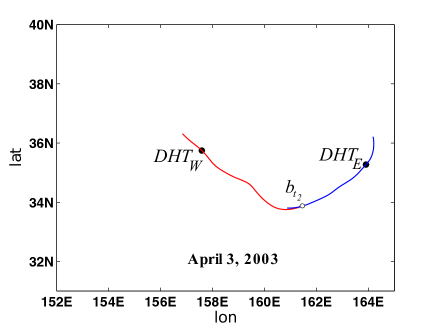
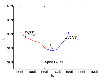
Figure 21: Boundaries at days April 3 2003 and April 17 2003 constructed from a (finite length) segment of the unstable manifold of DHT_W and a (finite length) segment of the stable manifold of DHT_E. The boundary intersection points are denoted respectively by $b_{t_{2}}$ and $b_{t_{4}}$. (Figure taken from Mendoza et al. (2010)).

Longer pieces of the same manifolds are represented in figure 22. Figure 22b) shows the asymptotic evolution on April 17 of the lobes represented in Figure 22a) on April 3. The green lobe area contains particles in the north on April 3 that eventually came to the south on April 17. Magenta particles that are analogously first in the south eventually come to the north on April 17.

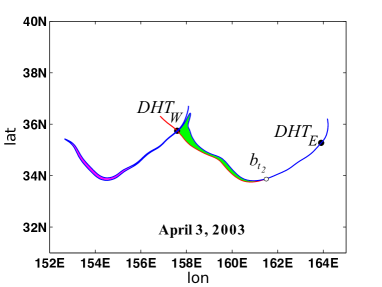
a)b)

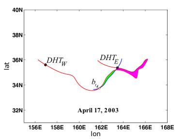
Figure 22: Turnstile lobes across the main stream at days April 3 and 17 2003. The magenta area evolves from south to north while the green area does from north to south. (Figure taken from Mendoza et al. (2010)).

Lobe dynamics across the main stream may be identified until 26 May 2003. On this date, DHT_W has lost its distinguished property and the reference point on the unstable manifold has disappeared. Mendoza et al. (2010) have reported that it is possible to identify a new reference point on the manifold, which is given by DHT${}_{W}^{+}$. The manifold is not asymptotic to DHT${}_{W}^{+}$. However, DHT${}_{W}^{+}$ marks a Distinguished Trajectory on the manifold with certain accuracy $\epsilon$.

The active transport mechanisms just described are simultaneous in time and the full description of transport routes should address how their action over ocean particles is combined. A complete representation of coincident events in Figure 23 reveals intersections between the lobe that is outside the eddy (magenta colour in Fig. 20a) on April 3, and the lobe which at the same time is located to the north of the barrier (green colour in Fig. 22a). The intersection area in grey colour, as shown in Figure 23 for April 3, provides dual information on the particles contained therein. It shows that those particles were inside the eddy on March 19 (as indicated in Figure 19 ) and were to be at the south of the Lagrangian barrier across the stream on April 17 (see Figure 22). Further similar intersections take place between the magenta lobes in the sequence displayed in Figure 20, and the sequence of lobes across the jet that transports water from north to south (see Mendoza et al. (2010) for a full description). Once particles reach the southern region, further interactions will take place with any dynamic structure covering the ocean surface in that area.

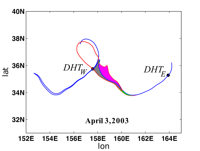
Figure 23: Intersection of lobes governing transport across the western eddy and those governing transport across the main stream of the Kuroshio current.

Additional complex routes may be traced for particles ejected from the western eddy. In fact, we are able to show that there is a non-zero flux from this eddy towards the eddy at the eastern limit. On April 16, Figure 24a) shows pieces of stable and unstable manifolds of the eddies at the west and east. The magenta coloured lobe represents the water ejected from the western eddy. There exists a non-zero intersection area between this lobe and the lobe regulating the water coming into the eastern eddy. The intersection area is depicted in dark grey. A remaining piece of the lobe penetrating on the eastern eddy is left in green. Figure 24 b) confirms the entrainment of this area on the eastern vortex on April 28.

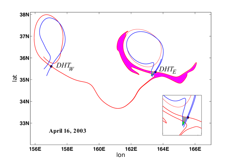
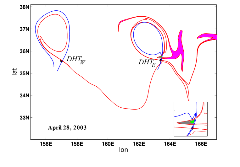
Figure 24: Intersection of lobes governing transport across the western and eastern eddies. a) On April 16 the grey area shows a portion of fluid ejected from the western eddy that will be entrained by the eastern eddy; b) on April 28 the grey area has come into the eastern eddy. Figures show insets with an amplification of the entrainment process.

A complete transport description would require connection of the information provided by all the dynamic structures tilling the ocean surface which are displayed by the function $M$ in Figure 7. However, in practice, providing thorough insights in terms of manifolds as discussed in this section is not always possible, because on the one hand it requires that the features of the observed dynamic patterns resemble those described in the mathematical literature, and on the other that they must have certain persistence in time. Rapidly transient regimes, such as those occurring in large areas of the analysed flow, are difficult to understand because they are related to changes in the topology of the flow that are not well interpreted from a dynamic point of view (see Mancho et al. (2008)). Related to these changes are mathematical issues such as non-uniform hyperbolicity, addressed for instance in (Barreira & Pesin, 2007), not yet completely understood for general non autonomous systems such as those represented by Eq. (1).

6 Conclusions

This article reports the combined used of several Lagrangian tools, some of them recently developed, and shows their success in obtaining extensive details about the description of purely advective transport events in arbitrary time dependent flows. We demonstrate the capabilities of these tools by analysing 2D data sets obtained from altimetric satellites over the Kuroshio Current.

We have first considered the evaluation of global Lagrangian descriptors over a general vector field. In particular we have chosen two types of descriptors, referred to as function $M$. Contour plots of these functions provide a time dependent phase portrait which is visualised by sharp changes in the colour code of $M$. These abrupt variations separate regions of trajectories with qualitatively different behaviours, and since this is exactly what invariant manifolds separate, boundaries of homogenous coloured areas position invariant manifolds. The dynamic picture provided by $M$ reveals at a glance the organising centres of the flow, hyperbolic and non-hyperbolic flow regions, invariant manifolds and jets. In other words it identifies the essential dynamical elements that must be considered by any kinematic model describing the exchange of trajectories on a given data set.

Although the dynamical structures are clearly visualised from $M$, a detailed description of transport requires the full identification of the organising trajectories, the Distinguished Hyperbolic Trajectories, and of their finite time stable and unstable manifolds. Our discussions are focused on 2D flows, although extension to higher dimensions are possible. Distinguished hyperbolic trajectories are computed by first examining $M$ as defined from Eq. (14), and identifying candidate areas which act as the organising centres of the flow. The search is completed by computing paths of limit coordinates on each recognised area for a full identification of the DHT positions. At a third stage, finite time stable and unstable manifolds of these DHTs are directly computed as advected curves. The algorithm starts with a small segment aligned either along the stable or the unstable subspace of the DHT, making this segment evolve either backwards or forwards in time respectively. Manifolds computed in this way become long intricate curves; transport details are obtained from them by selecting portions along the branches at both sides of the DHT. These selections allow transport routes across the ocean surface to be identified; for instance, masses of water penetrating or leaving an eddy, then of those masses protruding the eddy, parcels are identified crossing the main current or coming into a second eddy. A complete transport description connecting the information provided by all the dynamic structures tilling the ocean surface is foreseen. Despite the advances made, however a full transport description still remains a challenge because conceptual difficulties exist that are yet to be solved, especially when dealing with highly transient regimes in which the topology of the flow changes in time.

As a summary, we can say that our Lagrangian techniques have proven fluid exchange across the main current and between eddies in the Kuroshio region in a range of dates during the year 2003. This methodology constitutes an efficient tool of analysis for the uncountable data sets which nowadays are obtained from altimeter satellite or by other means. The performance of the machinery on the analyzed data opens a gateway to its applications in any kind of realistic flow for operational oceanography purposes and could be though as an alternative for the study of transport in oceanic flows to campaign measures based on quasi Lagrangian drifter releases.

Appendix A

We discuss here details about the numerical evaluation of $M$ as defined in Eq. (14). Trajectories $(x_{1}(t),x_{2}(t))$ of the system (11)-(12) are obtained numerically, and thus represented by a finite number of points, $L$. A discrete version of Eq. (14) is:

$$M=\sum_{j=1}^{L-1}\left(\int^{p_{f}}_{p_{i}}\!\!\!\sqrt{\left(\frac{dx_{1,j}(p)}{dp}\right)^{2}+\left(\frac{dx_{2,j}(p)}{dp}\right)^{2}}dp\right),$$ (48)

where the functions $x_{1,j}(p)$ and $x_{2,j}(p)$ represent a curve interpolation parametrised by $p$, and the integral

$$\int^{p_{f}}_{p_{i}}\!\!\!\sqrt{\left(\frac{dx_{1,j}(p)}{dp}\right)^{2}+\left(\frac{dx_{2,j}(p)}{dp}\right)^{2}}dp$$ (49)

is computed numerically. In accordance with the methodology described in (Madrid & Mancho, 2009), we use the interpolation method proposed by Dritschel (1989) in the context of contour dynamics. The interpolation equation, later used in this article, is given by expression (57). To compute the integral (49) we have used the Romberges method (see Press et al. (1992)) of order $2K$ where $K=5$. In the results reported in this article we have used this technique to evaluate Eq. (14). Another possibility for evaluating Eq. (49), which is less accurate but simpler and faster, is to approach it by the length of the linear segments linking successive points of the trajectory. In order to evaluate Eq. (15) where $\mathcal{F}({\bf x}(t))$ depends not only on velocity but also on other vectors such as acceleration, the time derivative of acceleration or their combinations, we propose a more versatile method which is easily adapted for any choice of $\mathcal{F}$. For instance, in the case where $\mathcal{F}({\bf x}(t))=|{\bf v}({\bf x}(t),t)|$, the integral in Eq. (15) evaluates the area $A$ below the graph $|{\bf v}({\bf x}(t),t)|$ in the referred time interval. In order to evaluate $A$ we consider the integral as the following one-dimensional dynamical system:

$$\frac{dY}{dt}=|{\bf v}({\bf x}(t),t)|.$$ (50)

For the initial condition $Y(t^{*})=0$, the area $A$ is provided by the value of $Y$ at $t^{*}+\tau$ minus the value of $Y$ at $t^{*}-\tau$ , i.e., $Y(t^{*}+\tau)-Y(t^{*}-\tau)=A$. The integration of the system (50) is performed with a 5th order variable time step Runge-Kutta method, in particular with the subroutine rkqs described in Press et al. (1992). The peculiarity of this differential equation is that it depends on $t$ both explicitly and implicitly (through the trajectory), and expressions such as the right hand side of the system (11)-(12) only provide the explicit dependence ${\bf v}({\bf x},t)$. A Runge Kutta step from $t_{0}$ to $t_{1}$ applied to Eq. (50) requires the evaluation of $|{\bf v}|$ along trajectories at intermediate steps $t_{0}+\Delta t$. To this end the argument ${\bf x}$ that must be passed to $|{\bf v}|$ at time $t_{0}+\Delta t$ must be obtained by evolving the trajectory from ($t_{0},{\bf x}(t_{0})$) to ($t_{0}+\Delta t,{\bf x}(t_{0}+\Delta t)$) according to the system (11)-(12). This method is quite adaptable, since from one descriptor to another it is only the right hand side in Eq. (50) which needs to be modified. This is the technique used for the case in which $\mathcal{F}({\bf x}(t))=|{\bf a}({\bf x}(t),t)|$, for which we report results.

Appendix B

We provide full details of the equations and algorithms used to compute the unstable manifolds. At each time $t_{k}$ in a discrete set of time increments $[t_{k},k=0...N]$, the unstable manifold is represented by a discrete set of points ${\bf x}_{j}$. In particular at time $t_{0}$ it is a small segment aligned along the unstable subspace of the hyperbolic trajectory, represented by five points. They are evolved along trajectories until time $t_{1}$, and each point is considered to leave unacceptable gaps with its neighbors if the measure $\sigma_{j}>1$. Here $\sigma_{j}=d_{j}\rho_{j}$ where $d_{j}={\bf x}_{j+1}-{\bf x}_{j}$ and $\rho_{j}$ is a density defined as follows:

$$\rho_{j}\equiv\frac{(\bar{\kappa}_{j}L)^{\frac{1}{2}}}{\mu L}+\bar{\kappa}_{j},$$ (51)

or $2/\zeta$, whichever is smaller. Here $\zeta$ serves as a small-scale cut-off distance for resolving manifold details which we have fixed to $10^{-6}$ and $L$ is a typical length scale fixed to 3. The parameter $\mu$ controls the overall point density along the manifold and needs tuning for individual problems. Small values of $\mu$ correspond to a high point density. In our computations it is fixed to 0.005. The quantity $\bar{\kappa}_{j}$ in (51) is defined in terms of $\check{\kappa}$,

$${\bar{\kappa}_{j}} \equiv(\check{\kappa}_{j}+\check{\kappa}_{j+1})/2,$$ (52)

which in turn is defined by

$$\check{\kappa}_{j} =\frac{w_{j-1}\tilde{\kappa}_{j-1}+w_{j}\tilde{\kappa}_{j}}{w_{j-1}+w_{j}},$$ (53)

which uses the weighting $$w_{j}=d_{j}/(d_{j}^{2}+4\zeta^{2}) \tilde{\kappa}_{j}$$ and the further curvature , which itself is defined by

$$\tilde{\kappa}_{j} =\sqrt{\kappa_{j}^{2}+1/L^{2}},$$ (54)

where $\kappa_{j}$, finally, is the local curvature:

$$\kappa_{j}=2\frac{a_{j-1}b_{j}-b_{j-1}a_{j}}{|d_{j-1}^{2}{\mathbf{t}}_{j}+d_{j}^{2}{\mathbf{t}}_{j-1}|}.$$ (55)

Here

$${\mathbf{t}}_{j} =(a_{j},b_{j})={{\mathbf{x}}}_{j+1}-{{\mathbf{x}}}_{j}, \qquad{t}_{j}\in{\mathbb{R}}^{2}$$ (56)

When a gap between nodes at time $t_{1}$ is too large, it is filled by inserting a point between the same nodes at $t_{0}$. The point is computed by interpolating with $p=0.5$ along the curve that links the points ${\bf x}_{j+1},{\bf x}_{j}$:

$${\mathbf{x}}(p)={\mathbf{x}}_{j}+p~{}{\mathbf{t}}_{j}+{\eta}_{j}(p)~{}{\mathbf{n}}_{j},$$ (57)

where ${\mathbf{t}}_{j}$ is given by Eq. (56) and:

$${\mathbf{n}}_{j} =(-b_{j},a_{j}), \qquad{n}_{j}\in{\mathbb{R}}^{2}$$ (58)

$${\eta}_{j}(p) =\mu_{j}p+\beta_{j}p^{2}+\gamma_{j}p^{3}, \qquad{\eta}_{j}(p)\in{\mathbb{R}}.$$ (59)

The cubic interpolation coefficients $\mu_{j}$, $\beta_{j}$ and $\gamma_{j}$ are:

$$\mu_{j} =-\frac{1}{3}d_{j}\kappa_{j}-\frac{1}{6}d_{j}\kappa_{j+1},$$ (60)

$$\beta_{j} =\frac{1}{2}d_{j}\kappa_{j},$$ (61)

$$\gamma_{j} =\frac{1}{6}d_{j}(\kappa_{j+1}-\kappa_{j}),$$ (62)

Once the manifold satisfies gap size acceptability condition at every node, i.e. $d_{j}\rho_{j}=\sigma_{j}<1$, the point redistribution algorithm is applied. This is useful to eliminate points in regions of the manifold where they may have accumulated Mancho et al. (2004). This algorithm is described in (Dritschel, 1989) and it works as we describe next. Let $n$ be the number of nodes at $t_{1}$:

$$q=\sum_{j=1}^{n}\sigma_{j}$$ (63)

and define $\tilde{n}=[q]+2$ (i.e., two more than the nearest integer to $q$). During redistribution the end points of the manifold are held fixed. The $n-2$ “old” nodes between the end points will be replaced by $\tilde{n}-1$ entirely new nodes in such a way that the spacing of new nodes is approximately consistent with the desired average density, controlled by the parameter $\mu$. Let $\sigma_{j}^{\prime}=\sigma_{j}\tilde{n}/q$ so that $\sum_{j=1}^{n}\sigma_{j}^{\prime}=\tilde{n}$. Then, the positions of the new nodes $i=2,...,\tilde{n}$ are found succesively by seeking for each successive $j$ a $p$ such that,

$$\sum_{l=1}^{j-1}\sigma_{l}^{\prime}+\sigma_{j}^{\prime}p=i-1,$$ (64)

and placing each new node $i$ between the old nodes $j$ and $j+1$ at the position ${\mathbf{x}}(p)$ given in (57).

References

- Aurell et al. (1997) Aurell, E., Boffetta, G., Crisanti, A., Paladin, G. & Vulpiani, A. 1997 Predictability in the large: an extension of the concept of lyapunov exponent. J. Phys. A 30, 1–26.
- B. A. Mosovsky (2011) B. A. Mosovsky, J. D. Meiss 2011 Transport in transitory dynamical systems. SIAM Journal on Applied Dynamical Systems 10, 35–65.
- Barreira & Pesin (2007) Barreira, L. & Pesin, Ya. 2007 Nonuniform hyperbolicity. In Encyclopedia Math. Appl. vol 115. Cambridge University Press.
- Beron-Vera et al. (2010) Beron-Vera, F. J., Olascoaga, M. J. & Goni, G. J. 2010 Surface ocean mixing inferred from multisatellite altimetry measurements. J. Phys. Oceanogr 40, 2466–2480.
- Branicki et al. (2011) Branicki, M., Mancho, A. M. & Wiggins, S. 2011 A lagrangian description of transport associated with a front-eddy interaction: application to data from the north-western mediterranean sea. Physica D 240, 282–304.
- Branicki & Wiggins (2009) Branicki, M. & Wiggins, S. 2009 An adaptive method for computing invariant manifolds in non-autonomous, three-dimensional dynamical systems. Physica D 238, 1625–1657.
- Branicki & Wiggins (2010) Branicki, M. & Wiggins, S. 2010 Finite-time lagrangian transport analysis: stable and unstable manifolds of hyperbolic trajectories and finite-time lyapunov exponents. Nonlinear Processes in Geophysics 17, 1–36.
- de la Cámara et al. (2012) de la Cámara, A., Mancho, A. M., Ide, K., Serrano, E. & Mechoso, C. R. 2012 Routes of transport across the antarctic polar vortex in the southern spring. Journal of the Atmospheric Sciences 69, 753–767.
- de la Cámara et al. (2010) de la Cámara, A., Mechoso, C. R., Ide, K., Walterscheid, R. & Schubert, G. 2010 Polar night vortex breakdown and large-scale stirring in the southern stratosphere. Climate Dynamics 35, 965–975.
- Cencini et al. (1999) Cencini, M., Lacorata, G., Vulpiani, A. & Zambianchi, E. 1999 Mixing in a meandering jet: a markovian approximation. J. Phys. Oceanography 29, 2578 2594.
- Coulliette & Wiggins (2001) Coulliette, C. & Wiggins, S. 2001 Intergyre transport in a wind-driven, quasigeostrophic double gyre: an application of lobe dynamics. Nonlin. Processes Geophys. 8, 69–94.
- d’Ovidio et al. (2009) d’Ovidio, F., Isern-Fontanet, J., López, C., Garc a-Ladona, E. & Hernández-García, E. 2009 Comparison between eulerian diagnostics and the finite-size lyapunov exponent computed from altimetry in the algerian basin. Deep Sea Res. I 56, 15–31.
- Dritschel & Ambaum (1997) Dritschel, D.G. & Ambaum, M.H.P. 1997 A contour-advective semi-lagrangian numerical algorithm for simulating fine-scale conservative dynamical fields. Quart. J. Roy. Meteor. Soc. 123, 1097–1130.
- Dritschel (1989) Dritschel, D. G. 1989 Contour dynamics and contour surgery: numerical algorithms for extended, high-resolution modelling of vortex dynamics in two-dimensional, inviscid, incompressible flows. Comput. Phys. Rep. 10, 77–146.
- Duan & Wiggins (1996) Duan, J.Q. & Wiggins, S. 1996 Fluid exchange across a meandering jet with quasiperiodic time variability. J. Phys. Oceanography 26, 1176–1188.
- Farazmand & Haller (2012) Farazmand, M. & Haller, G. 2012 Computing lagrangian coherent structures from their variational theory. Chaos 22, 013128.
- Haller (2001) Haller, G. 2001 Distinguished material surfaces and coherent structures in three-dimensional fluid flows. Physica D 149, 248–277.
- Hernández-Carrasco et al. (2011) Hernández-Carrasco, I., Hernández-García, E., López, C. & Turiel., A. 2011 How reliable are finite-size lyapunov exponents for the assessment of ocean dynamics? Ocean Modelling 36, 208–218.
- Ide et al. (2002) Ide, K., Small, D. & Wiggins, S. 2002 Distinguished hyperbolic trajectories in time-dependent fluid flows: analytical and computational approach for velocity fields defined as data sets. Nonlin. Processes Geophys. 9, 237–263.
- Joseph & Legras (2002) Joseph, B. & Legras, B. 2002 Relation between kinematic boundaries, stirring, and barriers for the antarctic polar vortex. J. of the Atmospheric Sciences 59, 1198–1212.
- Ju et al. (2003) Ju, N., Small, D. & Wiggins, S. 2003 Existence and computation of hyperbolic trajectories of aperiodically time dependent vector fields and their approximations. Int. J. Bifurcation Chaos Appl. Sci. Eng. 13, 1449–1457.
- Kuznetsov et al. (2002) Kuznetsov, L., Toner, M., Kirwan, A. D. & Jones, C.K.R.T 2002 The loop current and adjacent rings delineated by lagrangian analysis of the near-surface flow. J. of Marine Research 60, 405–429.
- Larnicol et al. (2006) Larnicol, G., Guinehut, S., Rio, M. H., Drevillon, M., Faugere, Y. & Nicolas, G. 2006 The global observed ocean products of the french mercator project. Proceedings of the 15 years of progress in Radar altimetry, ESA symposium, Venice, March .
- Lehahn et al. (2007) Lehahn, Y., d’Ovidio, F., Levy, M. & Heifetz, E. 2007 Stirring of the northeast atlantic spring bloom: a lagrangian analysis based on multi-satellite data. J. Geophys. Res. 112, C08005.
- Madrid & Mancho (2009) Madrid, J. A. J. & Mancho, A. M. 2009 Distinguished trajectories in time dependent vector fields. Chaos 19, 013111.
- Malhotra et al. (1998) Malhotra, N., Mezic, I. & Wiggins, S. 1998 Patchiness: A new diagnostic for lagrangian trajectory analysis in time-dependent fluid flows. International Journal of Bifurcation and Chaos 8, 1053–1093.
- Malhotra & Wiggins (1998) Malhotra, N. & Wiggins, S. 1998 Geometric structures, lobe dynamics, and lagrangian transport in flows with aperiodic timedependence, with applications to rossby wave flow. J. Nonlin. Science 8, 401–456.
- Mancho et al. (2008) Mancho, A. M., Hernández-García, E., Small, D. & Wiggins, S. 2008 Lagrangian transport through an ocean front in the northwestern mediterranean sea. J. of Physical Oceanography 38, 1222–1237.
- Mancho & Mendoza (2011) Mancho, A. M. & Mendoza, C. 2011 The phase portrait of aperiodic non-autonomous dynamical systems. http://arxiv.org/abs/1106.1306 pp. 1–35.
- Mancho et al. (2004) Mancho, A. M., Small, D. & Wiggins, S. 2004 Computation of hyperbolic and their stable and unstable manifolds for oceanographic flows represented as data sets. Nonlin. Processes Geophys. 11, 17–33.
- Mancho et al. (2006a) Mancho, A. M., Small, D. & Wiggins, S. 2006a A comparison of methods for interpolating chaotic flows from discrete velocity data. Comp. & Fluids 35, 416–428.
- Mancho et al. (2006b) Mancho, A. M., Small, D. & Wiggins, S. 2006b A tutorial on dynamical systems concepts applied to lagrangian transport in oceanic flows defined as finite time data sets: Theoretical and computational issues. Phys. Rep. 437, 55–124.
- Mancho et al. (2003) Mancho, A. M., Small, D., Wiggins, S. & Ide, K. 2003 Computation of stable and unstable manifolds of hyperbolic trajectories in two-dimensional, aperiodically time-dependent vector fields. Physica D 182, 188–222.
- Mendoza & Mancho (2010) Mendoza, C. & Mancho, A. M. 2010 The hidden geometry of ocean flows. Phys. Rev. Lett. 105, 038501–1–038501–4.
- Mendoza et al. (2010) Mendoza, C., Mancho, A. M. & Rio, M. H. 2010 The turnstile mechanism across the kuroshio current: analysis of dynamics in altimeter velocity fields. Nonlin. Processes Geophys. 17, 103–111.
- Meyers (1994) Meyers, S.D. 1994 Cross-frontal mixing in a meandering jet. J. Phys. Oceanography 24, 1641–1646.
- Mezić et al. (2010) Mezić, I., Loire, S., Fonoberov, V.A. & Hogan, P. 2010 A new mixing diagnostic and gulf oil spill movement. Science 330, 486–489.
- Miller et al. (2002) Miller, P. D., Pratt, L. J., Helfrich, K.R., Jones, C.K.R.T, Kanth, L.H. & Choi, J. 2002 Chaotic transport of mass and potential vorticity for an island recirculation. J. of Physical Oceanography 32, 80–102.
- Nese (1989) Nese, J. M. 1989 Quantifying local predictability in phase space. Physica D 35, 237–250.
- Poje et al. (1999) Poje, A.C., Haller, G. & Mezic, I. 1999 The geometry and statistics of mixing in aperiodic flows. Physics of Fluids 11, 2963–2968.
- Press et al. (1992) Press, W. H., Teukolsky, S. A., Vetterling, W.T. & Flannery, B. P. 1992 In Numerical recipes in C (ed. L. Cowles & A. Harvey), p. 1256. Cambridge University Press.
- Rio & Hernandez (2003) Rio, M. H. & Hernandez, F. 2003 High-frequency response of wind-driven currents measured by drifting buoys and altimetry over the world ocean. J. Geophysical Research-Oceans 108, 3283.
- Rio & Hernandez (2004) Rio, M. H. & Hernandez, F. 2004 A mean dynamic topography computed over the world ocean from altimetry, in situ measurements, and a geoid model. J. Geophysical Research-Oceans 109, C12032.
- Rio et al. (2005) Rio, M. H., Schaeffer, P., Hernandez, F. & Lemoine, J. 2005 The estimation of the ocean mean dynamic topography through the combination of altimetric data, in-situ measurements and grace geoid: From global to regional studies. Proceedings of the GOCINA International Workshop, Luxemburgo .
- Rogerson et al. (1999) Rogerson, A. M., Miller, P. D., Pratt, L. J. & Jones, C.K.R.T 1999 Lagrangian motion and fluid exchange in a barotropic meandering jet. J. of Physical Oceanography 29, 2635–2655.
- Rom-Kedar et al. (1990) Rom-Kedar, V., Leonard, A. & Wiggins, S. 1990 An analytical study of transport, mixing, and chaos in an unsteady vortical flow. J. Fluid Mech. 214, 347–394.
- Rypina et al. (2011) Rypina, I. I., Scott, S. E., Pratt, L. J. & Brown, M. G. 2011 Investigating the connection between complexity of isolated trajectories and lagrangian coherent structures. Nonlinear Processes in Geophysics 18, 977–987.
- S. Dutkiewicz (1993) S. Dutkiewicz, A. Griffa, D.B. Olson 1993 Particle diffusion in a meandering jet. J. Geophys. Res. 98, 16487 16500.
- Samelson (1992) Samelson, R.M. 1992 Fluid exchange across a meandering jet. J. Phys. Oceanography 22, 431–440.
- Samelson & Wiggins (2006) Samelson, R. & Wiggins, S. 2006 Interdisciplanary applied mathematics, geophysics and planetary sciences. In Lagrangian Transport in Geophysical Jets and Waves (ed. S. S. Antman & J. E. Marsden), p. 145. Springer.
- Shadden et al. (2005) Shadden, S. C., lekien, F. & Marsden, J. 2005 Definition and properties of lagrangian coherent structures from finite-time lyapunov exponents in two-dimensional aperiodic flows. Physica D 212, 271–304.
- Turiel et al. (2009) Turiel, A., Nieves, V., García-Ladona, E., Font, J., Rio, M.-H. & Larnicol, G. 2009 The multifractal structure of satellite sea surface temperature maps can be used to obtain global maps of streamlines. Ocean Science 5, 447–460.
- Waugh & Abraham (2008) Waugh, D.W. & Abraham, E.R. 2008 Stirring in the global surface ocean. Geophys. Res. Lett. 35, L20605.
- Wiggins (1992) Wiggins, S. 1992 Interdisciplanary applied mathematics. In Chaotic Transport in Dynamical Systems, p. 301. Springer-Verlag.