Cosmological Constraints on the Undulant Universe

Abstract

We use the redshift Hubble parameter $H(z)$ data derived from relative galaxy ages, distant type Ia supernovae (SNe Ia), the Baryonic Acoustic Oscillation (BAO) peak, and the Cosmic Microwave Background (CMB) shift parameter data, to constrain cosmological parameters in the Undulant Universe. We marginalize the likelihood functions over $h$ by integrating the probability density $P\propto e^{-\chi^{2}/2}$. By using the Markov Chain Monte Carlo (MCMC) technique, we obtain the best fitting results and give the confidence regions on the $b-\Omega_{\rm m0}$ plane. Then we compare their constraints. Our results show that the $H(z)$ data play a similar role with the SNe Ia data in cosmological study. By presenting the independent and joint constraints, we find that the BAO and CMB data play very important roles in breaking the degeneracy compared with the $H(z)$ and SNe Ia data alone. Combined with the BAO or CMB data, one can improve the constraints remarkably. The SNe Ia data sets constrain $\Omega_{\rm m0}$ much tighter than the $H(z)$ data sets, but the $H(z)$ data sets constrain $b$ much tighter than the SNe Ia data sets. All these results show that the Undulant Universe approaches the $\Lambda\rm$CDM model. We expect more $H(z)$ data to constrain cosmological parameters in future.

1 Introduction

Many cosmological observations (Bennett et al. (2003); Spergel et al. (2007); Eisenstein et al. (2005); Kowalski et al. (2008)), such as distant SNe Ia (Riess et al. (1998); Perlmutter et al. (1999)), the subsequent CMB measurement by Wilkinson Microwave Anisotropy Probe (WMAP) (Spergel et al. (2003)) and the large scale structure survey by Sloan Digital Sky Survey (SDSS) (Tegmark et al. (2004a); Tegmark et al. (2004b)) etc. support that our Universe is undergoing an accelerated expansion, and these data have mapped the universe successfully by constraining cosmological parameters (Perlmutter et al. (1999); Tegmark et al. (2000); Zhu (2004); Zhan et al. (2006); Lineweaver (1998); Efstathiou (1999); Zhan et al. (2005); Maartens et al. (2006)). Meanwhile, many different observations, such as the redshift-dependent quantities, are used usually. The luminosity distance to a particular class of objects, e.g. SNe Ia and Gamma-Ray Bursts (GRBs) (Nesseris & Perivolaropoulos (2004)), the size of the BAO peak detected in the large-scale correlation function of luminous red galaxies from SDSS (Eisenstein et al. (2005)) and the CMB data obtained from the three-year WMAP estimate (Wang & Mukherjee (2006); Spergel et al. (2007)) are redshift-dependent. The BAO and CMB data have been combined to constrain the cosmological parameters widely. Recently, the Hubble expansion rate at different redshifts can be obtained from the measurement of relative galaxy ages directly. As a function of redshift $z$, the $H(z)$ data have been used to test cosmological models (Gong et al. (2008); Yi & Zhang (2007); Samushia & Ratra (2006); Wei & Zhang (2007); Zhang et al. (2007); Wei & Zhang (2007); Zhang & Wu (2007); Dantas et al. (2007); Zhang & Zhu (2007); Wu & Yu (2007); Wei & Zhang (2007)). Using different data to constrain parameters can provide the consistency checks between each other, and the combination of different data can also make the constraints tighter (Li et al. (2008); Zhao et al. (2007); Xia et al. (2006)). So far, few work has been done in comparison. We’d like to study the comparison of the SNe Ia, $H(z)$, BAO and CMB data in this letter. Although lots of cosmological models, e.g. the Quintessence (Caldwell et al. (1998)), the brane world (Deffayet et al. (2002)), the Chaplygin Gas (Alcaniz et al. (2003)) and the holographic dark energy models (Ke & Li (2005)), are extensively explored to explain the acceleration of the universe. $\Lambda\rm$CDM model, which is a standard and popular model, has been studied by Lin et al. (Lin et al. (2008)). In fact, there are some problems in the standard model, and this model is not consistent with the real universe. Scientists proposed a Undulant Universe, which is characterized by alternating periods of acceleration and deceleration (Gabriela (2005)). This model can remove the fine tuning problem (Vilenkin (2001); Jaume et al. (1999); Bludman (2000); Garriga & Vilenkin (2001); Stewart (2000)), and solve the coincidence scandal between the observed vacuum energy and the current matter density, with some details in (Peebles & Ratra (2003)). The equation of state (EOS) of the Undulant Universe is

$$\omega(a)=-\cos(\rm b\ln a),$$ (1)

where the dimensionless parameter $b$ controls the frequency of the accelerating epochs. Due to most inflation models predicting $\Omega_{\rm k}<10^{-5}$ (Tegmark & Rees (1998)), we assume spatial flatness, so the Hubble parameter is

$$H^{2}(a)=H_{0}^{2}(\Omega_{\rm m0}a^{-3}+\Omega_{\Lambda 0}a^{-3}\exp[\frac{3}{b}\sin(b\ln a)]),$$ (2)

where $\Omega_{\rm m0}$, $\Omega_{\Lambda 0}$ are the density parameter of matter and dark energy, respectively. Furthermore, S. Nesseris and L. Perivolaropoulos have enhanced the fact that an oscillating expansion rate ansatz has provided the best fit to the data among many ansatz by using recent supernova data(Nesseris & Perivolaropoulos (2004)).

In this letter, we concentrate on the comparison of different data sets on the Undulant Universe. In §ii@, we simply introduce these data sets that we use. Then the constraints are shown in §iii@. Finally, we show some important conclusions and discussions in §iv@.

2 Observational data

2.1 SNe Ia data

There has been some calibrated SNe Ia data with high confidence in (Kowalski et al. (2008)). This data set contains 307 data and the redshifts of these data span from about 0.01 to 1.75. These data give luminosity distances $d_{\rm L}(z_{i})$ and the redshifts $z_{i}$ of the corresponding SNe Ia. In a Friedmann-Robertson-Walker (FRW) cosmology, considering a flat universe, the luminosity distance is,

$$d_{\rm L}(z)=\frac{c(1+z)}{H_{0}}{\mathcal{F}}(z),$$ (3)

The function ${\mathcal{F}}(z)$ is defined as ${\mathcal{F}}(z)=\int_{0}^{z}{\rm d}z/E(z)$, with $E(z)=H(z)/H_{0}=\sqrt{\Omega_{M0}a^{-3}+\Omega_{\Lambda 0}a^{-3}\exp[\frac{3}{b}\sin(b\ln a)]}$. $H_{0}$ is the Hubble constant. The distance modulus is

$$\mu(z)=\rm m-\rm M=5\log\frac{d_{\rm L}}{10{\rm pc}}=42.39+5\log\ \frac{1+z}{h}{\mathcal{F}}(z),$$ (4)

with $h=H_{0}/100$ km s^-1 Mpc ^-1, where $\rm m$ and $\rm M$ are the apparent and absolute magnitudes, respectively.

2.2 The BAO Data

As the acoustic oscillations in the relativistic plasma of the early universe will also be imprinted onto the late-time power spectrum of the non-relativistic matter (Eisenstein & Hu (1998)), the acoustic signatures in the large-scale clustering of galaxies yield additional tests for cosmology (Spergel et al. (2003)). Eisenstein et al. (Eisenstein et al. (2005)) choose a spectroscopic sample of 46748 luminous red galaxies from SDSS to find the peaks successfully. These galaxies cover 3816 square degrees and have been observed at redshifts up to $z=0.47$. The peaks are described by the model-independent $\mathcal{A}$-parameter. $\mathcal{A}$-parameter is independent of Hubble constant $H_{0}$,

$$\mathcal{A}=\frac{\sqrt{\Omega_{\rm m}}}{z_{1}}[\frac{z_{1}}{E(z_{1})}\mathcal{F}^{2}(z_{1}))]^{1/3},$$ (5)

where $z_{1}=0.35$ is the redshift at which the acoustic scale has been measured. Eisenstein et al. suggested that the measured value of the $\mathcal{A}$-parameter is $\mathcal{A}=0.469\pm 0.017$ (Eisenstein et al. (2005)).

2.3 The CMB Data

The expansion of the Universe has transformed the black body radiation, which is left over from the Big Bang, into the nearly isotropic 2.73 K cosmic microwave background (CMB) (Bernardis et al. (2000)). The whole shift of the CMB angular power spectrum is determined by the CMB shift parameter $\mathcal{R}$. The shift parameter perhaps the most model-independent parameter, is also independent of $H_{0}$. It can be derived from CMB data (Bond et al. (1997); Odman et al. (2003)),

$$\mathcal{R}=\sqrt{\Omega_{\rm m}}\mathcal{F}(z_{\rm r}),$$ (6)

where $z_{\rm r}=1089$ is the redshift of recombination. Using the Markov Chain Monte Carlo (MCMC) chains from the analysis of the three-year results of WMAP (Spergel et al. (2007)), Wang & Mukherjee compute the CMB shift parameter to get $\mathcal{R}=1.70\pm 0.03$ and demonstrate that its measured value is mostly independent of assumptions about dark energy (Wang & Mukherjee (2006)).

2.4 the $H(z)$ data from relative galaxy ages

The Hubble parameter $H(z)$ data can be derived from the derivative of redshift $z$ with respect to the cosmic time $t$, i.e. ${\rm d}z/{\rm d}t$ (Jimenez & Loeb (2002)),

$$H(z)=-\frac{1}{1+z}\frac{{\rm d}z}{{\rm d}t}.$$ (7)

Therefore, an application of the differential age method to old elliptical galaxies in the local universe can determine the value of the current Hubble constant. This is a direct measurement for $H(z)$ through a determination of ${\rm d}z/{\rm d}t$. Jimenez et al. (Jimenez et al. (2003)) have applied the method to a $z\leq 0.2$ sample. Paying careful attention to uncertainties in the distance, systematics, and model uncertainties, they have selected Monte-Carlo techniques to demonstrate the feasibility by evaluating the errors. They also use many other different methods and yield consistent value for the Hubble constant. Hence, the $H(z)$ data are reliable. With the availability of new galaxy surveys, it becomes possible to determine $H(z)$ at $z>0$. By using the differential ages of passively evolving galaxies determined from the Gemini Deep Deep Survey (GDDS) (Abraham et al. (2004)) and archival data (Treu et al. (2001); Treu et al. (2002); Nolan et al. (2003a); Nolan et al. (2003b)), Simon et al. derive a set of $H(z)$ data, which is listed in Table.1 (Simon et al. (2005), see also Samushia & Ratra (2006); Jimenez et al. (2003)). The estimation method in detail can be found in the work (Simon et al. (2005)). As $z$ has a relatively wide range, $0.1<z<1.8$, these data are expected to provide a full-scale description for the dynamical evolution of our universe. The application of the $H(z)$ data to cosmology can be referred to (Simon et al. (2005); Yi & Zhang (2007); Samushia & Ratra (2006); Wei & Zhang (2007); Lin et al. (2008); Gong et al. (2008)) and so on.

Table 1: the $H(z)$ data in units of km s^-1Mpc^-1 (Simon et al. (2005)) (see Samushia & Ratra (2006); Jimenez et al. (2003) also)

$z$(redshift)	0.09	0.17	0.27	0.40	0.88	1.30	1.43	1.53	1.75
$H(z)$	69	83	70	87	117	168	177	140	202
1$\sigma$ error	12.0	8.3	14.0	17.4	23.4	13.4	14.2	14.0	40.4

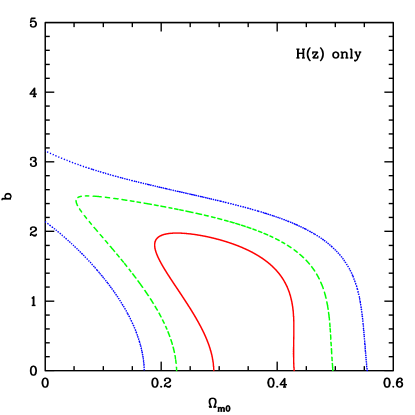
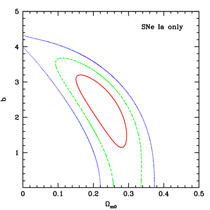
Figure 1: The contour maps of $b-\Omega_{\rm m0}$ for different data sets. The left panel is $H(z)$ only, and the right panel is SNe Ia only. Confidence regions are at $68.3\%$, $95.4\%$ and $99.7\%$ levels from inner to outer respectively, for a flat Undulant Universe without a prior of $h$.

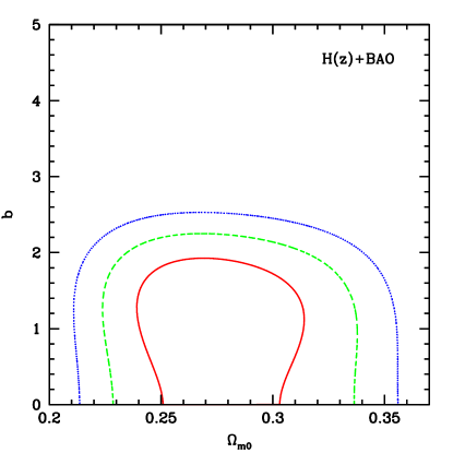
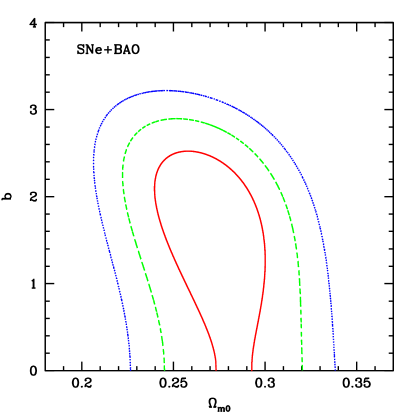
Figure 2: The contour maps of $b-\Omega_{\rm m0}$ for different sets. The left panel is $H(z)$+BAO, and the right panel is SNe Ia+BAO. Confidence regions are at $68.3\%$, $95.4\%$ and $99.7\%$ levels from inner to outer respectively, for a flat Undulant Universe without a prior of $h$.

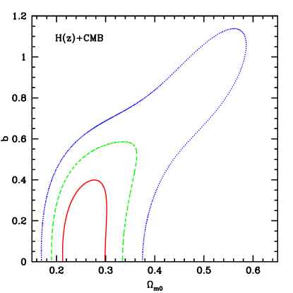
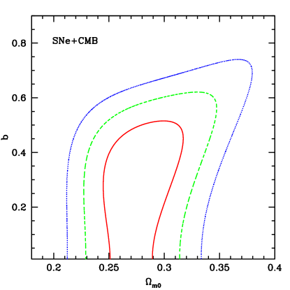
Figure 3: The contour maps of $b-\Omega_{\rm m0}$ for different sets. The left panel is $H(z)$+CMB, and the right panel is SNe Ia+CMB. Confidence regions are at $68.3\%$, $95.4\%$ and $99.7\%$ levels from inner to outer respectively, for a flat Undulant Universe without a prior of $h$.

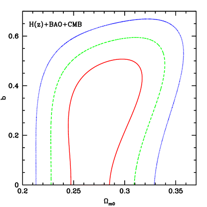
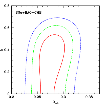
Figure 4: The contour maps of $b-\Omega_{\rm m0}$ for different sets. The left panel is $H(z)$+BAO+CMB, and the right panel is SNe Ia+BAO+CMB. Confidence regions are at $68.3\%$, $95.4\%$ and $99.7\%$ levels from inner to outer respectively, for a flat Undulant Universe without a prior of $h$.

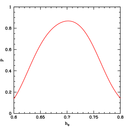
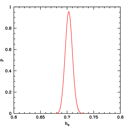
Figure 5: The probability distribution function of $h$ for $H(z)$ and SNe Ia data, respectively, for a flat Undulant Universe.

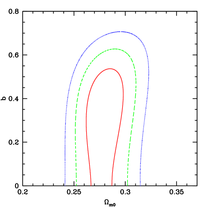
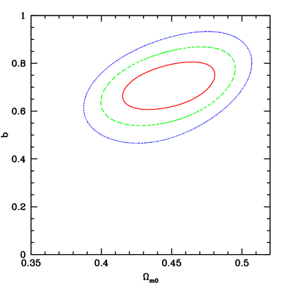
Figure 6: The contour maps of $b-\Omega_{\rm m0}$ for SNe Ia+BAO+CMB with a ”wrong” $h$ prior. $h$ is $0.7$ for the left panel, and $0.65$ for the right panel. Confidence regions are at $68.3\%$, $95.4\%$ and $99.7\%$ levels from inner to outer respectively, for a flat Undulant Universe without a prior of $h$.

3 Constraints on the Undulant Universe

Considering that the contents of the universe are mainly dark matter and dark energy, we just show $b-\Omega_{\rm m0}$ plane contour maps, where $b$ traces dark energy, and $\Omega_{\rm m0}$ traces dark matter respectively. We estimate the best fit to the set of parameters by using individual $\chi^{2}$ statistics, with

$$\chi^{2}_{\mid\rm data}=\sum^{\rm N}_{\rm i=1}\frac{[d^{\rm i}_{\rm t}(z)-d^{\rm i}_{\rm o}(z)]^{2}}{\sigma^{2}_{\rm i}},$$ (8)

where $\rm N$ is the number of data in each set, and $d^{\rm i}_{\rm t}(z)$ is the value at $z_{\rm i}$ given by above theoretical analysis. $d^{\rm i}_{\rm o}(z)$ is individual observational value in each data set at $z_{\rm i}$, and $\sigma_{\rm i}$ is the error due to uncertainties. In order to strengthen the constraints, we use MCMC technique to modulate the process (Gong et al. (2007)).

It is worth noting that the value of $h$ may strongly affect the constraint process, because the probability distribution function (PDF) of $h$ for each data is different. We can see the PDF for $H(z)$ and SNe Ia data in Fig.5. For $H(z)$ data, we find the PDF of $h$ covers a large range, while it is small for SNe Ia date. Because the distribution of $h$ constrained by SNe Ia is very narrow, if we fix $h$ far from the best-fit, then the constraints will be totally wrong.For example, we test the effect on fixing a ”wrong” $h$ by using SNe Ia+BAO+CMB. As can be seen in Fig.6, with a ”wrong” $h$ prior, the constraints of the left panel are very different from that of the right panel. This is because if we assume a ”wrong” prior for $h$, the $\chi^{2}$ would become very large ($\chi^{2}\sim 426$ for $h=0.65$ while $\chi^{2}\sim 312$ for $h=0.7$), and then we will get a false minimum $\chi^{2}$ to lead to a wrong result.However, if we marginalize the likelihood functions over $h$ by integrating the probability density $P\propto e^{-\chi^{2}/2}$, we can remove the effect of the distribution of $h$, and illustrate the reliable distribution of the other parameters. Therefore, we marginalize the likelihood functions over $h$ to obtain the best fitting results. Then we get the confidence regions and the $b-\Omega_{\rm m0}$ plane.

As it is seen from Eq.(1), $\omega(a)$ is an even function. Correspondingly, the values of $b$ are along the axis of $\Omega_{\rm m0}$ symmetrical distribution. Thus, the constraints on $b$ just in the range from $0$ to $+\infty$ are enough to demonstrate the comparison. Fig.1 shows the confidence regions determined by the $H(z)$ and SNe Ia data alone respectively. We find that the constraints on $\Omega_{\rm m0}$ from the $H(z)$ data are weaker than that from the SNe Ia data. Although we just have 9 data in $H(z)$ and 307 data in SNe Ia, there is still some consistency between them in the constraints. The joint constraints are shown in Fig.2, Fig.3, and Fig.4. We find that the constraints are weak if we use the $H(z)$ or SNe Ia data alone, however, after inclusion of the other observational data (the BAO or CMB data), the constraints are improved remarkably. Especially, the CMB data improve the constraints more remarkably. For breaking the degeneracy, the BAO and CMB data play very important roles in the constraint compared with the $H(z)$ and SNe Ia data alone. In the left contour map of Fig.1, and the two contour maps of Fig.2, Fig.3, and Fig.4, all contours at the $1\sigma$ confidence for $b$ are open-ended. It shows that $b$ takes possible value around $0$. We have not demonstrated the details of the constraints, because MCMC technique cannot determine exact values reliably. These contours correspond to $1\sigma,2\sigma$, and $3\sigma$ confidence from inside to outside. Table.2 summarizes $68.3\%$ confidence intervals. From the table, we find that the constraints on $\Omega_{\rm m0}$ from $H(z)$+BAO are looser than that from SNe Ia+BAO, and there is little difference between them. However, the constraints on $b$ from SNe Ia+BAO are looser than that from $H(z)$+BAO. The similar conclusions can be derived from comparing $H(z)$+CMB with SNe Ia+CMB, and $H(z)$+BAO+CMB with SNe Ia+BAO+CMB. The results of $\Omega_{\rm m0}$ on the Undulant Universe are consistent with the recent reported results from WMAP 5-year data (Kowalski et al. (2008)). The distribution of $b$ is close to $0$, i.e. the Undulant Universe approaches the $\Lambda\rm$CDM model. Comparing Fig.4 with Fig.6, we find that the result of the right panel in Fig.6 with $h=0.7$ is similar with that of the right panel in Fig.4 with marginalizing $h$, but has a smaller range for $\Omega_{\rm m0}$. On the other hand, from the result of the left panel in Fig.6 with $h=0.65$, we find that the range of $b$ shrinks to $0.6\sim 0.8$ at $68.3\%$ C.L. and the best-fit value of $\Omega_{\rm m0}$ moves to $\sim 0.45$ around, which are wrong results.

Table 2: $68.3\%$ confidence intervals for each observational data

Data	$H(z)$	SNe	$H(z)$+BAO	SNe+BAO
$\Omega_{m0}$	$[0.158,0.43]$	$[0.150,0.299]$	$[0.239,0.315]$	$[0.239,0.305]$
$b$	$[0,2.0]$	$[1.13,3.21]$	$[0,1.95]$	$[0,2.47]$
Data	$H(z)$+CMB	SNe+CMB	$H(z)$+BAO+CMB	SNe+BAO+CMB
$\Omega_{m0}$	$[0.21,0.30]$	$[0.244,0.318]$	$[0.244,0.318]$	$[0.253,0.304]$
$b$	$[0,0.40]$	$[0,0.53]$	$[0,0.51]$	$[0,0.58]$

4 Conclusions and Discussions

So far, we’ve presented some kinds of constraints on cosmological parameters by using the $H(z)$, SNe Ia, BAO and CMB data on the flat Undulant Universe, and we have marginalized the parameter $h$ to get the best fitting results. Because if we fix a ”wrong” prior for $h$, any model we take cannot fit the observational data, and then leads to a false $\chi^{2}$. We show confidence regions on the $b-\Omega_{\rm m0}$ plane. The Undulant model can trace the distribution of dark energy in undulant case. Therefore, our conclusions are more general. As discussed above, we have showed the comparison of different data sets carefully. Comparing with the $H(z)$ and SNe Ia data alone, the BAO and CMB data play very important roles in breaking the degeneracy. The constraints on $\Omega_{\rm m0}$ from the $H(z)$ data are looser than that from the SNe Ia data, but there is little difference between them. For the combined data sets, the constraints are improved remarkably. The CMB data improve the constraints more remarkably than the BAO data. In the joint constraints, the results from the $H(z)$ data sets ($H(z)$+BAO, $H(z)$+CMB and $H(z)$+BAO+CMB) are almost consistent with that from the SNe Ia data sets (SNe Ia+BAO, SNe Ia+CMB and SNe Ia+BAO+CMB). We find all the constraints on $b$ are around $0$, but the $H(z)$ data sets constrain $b$ more tightly. Namely, the Undulant Universe approaches the $\Lambda\rm$CDM model. However, on $\Omega_{\rm m0}$, the constraints of the $H(z)$ data sets are weaker than that of the SNe Ia data sets. It is probably because the data amount is not sufficient and the corresponding errors are very large (Samushia & Ratra (2006)). Only are there 9 $H(z)$ data in our discussion, but we still get such fine tight constraints. We speculate that the constraints of the $H(z)$ data sets will be tighter if we get more $H(z)$ data. Therefore, much more $H(z)$ data have an advantage over the SNe Ia data in the constraint. Fortunately, a large amount of $H(z)$ including data from the AGN and Galaxy Evolution Survey (AGES) and the Atacama Cosmology Telescope (ACT) are expected to be available in the next few years (Samushia & Ratra (2006)). Provided a statistical sample of many hundreds of galaxies, we could determine the value of $H(z)$ data to a percent accuracy. Paying attention to the assumption that SNe Ia is “standard candle”, it might make the luminosity distance $d_{L}$ of SNe Ia sample biased. In addition, there exists an integration of the inverse of $H(z)$ in $d_{L}$, and some uncertainties in the minimizing $\chi^{2}$ statistics might also arise from this integration. On the contrary, $H(z)$ do not suffer from this uncertainty resulting from integration. Therefore, the $H(z)$ data should constrain parameters more strongly than the SNe Ia data. We also notice that, the redshift range of $H(z)$ is from 0.09 to 1.75 and the redshift range of SNe Ia is from about 0.01 to 1.75. Thus, $H(z)$ and SNe Ia are distributed in the same range of redshift roughly. Therefore, the $H(z)$ data seem to provide us with an independent, very simple, and very powerful probe of fundamental cosmological parameters. With a large amount of the $H(z)$ data in the future, we probably can constrain cosmological parameters by using the $H(z)$ data instead of the SNe Ia data.