Numerical Methods for the Lévy LIBOR model

Abstract.

The aim of this work is to provide fast and accurate approximation schemes for the Monte-Carlo pricing of derivatives in the Lévy LIBOR model of EberleinOezkan05. Standard methods can be applied to solve the stochastic differential equations of the successive LIBOR rates but the methods are generally slow. We propose an alternative approximation scheme based on Picard iterations. Our approach is similar in accuracy to the full numerical solution, but with the feature that each rate is, unlike the standard method, evolved independently of the other rates in the term structure. This enables simultaneous calculation of derivative prices of different maturities using parallel computing. We include numerical illustrations of the accuracy and speed of our method pricing caplets.

1. Introduction

The LIBOR market model has become a standard model for the pricing of interest rate derivatives in recent years. The main advantage of the LIBOR model in comparison to other approaches, is that the evolution of discretely compounded, market-observable forward rates is modeled directly and not deduced from the evolution of unobservable factors. Moreover, the log-normal LIBOR model is consistent with the market practice of pricing caps according to Black’s formula (cf. Black76). However, despite its apparent popularity, the LIBOR market model has certain well-known pitfalls.

On the one hand, the log-normal LIBOR model is driven by a Brownian motion, hence it cannot be calibrated adequately to the observed market data. An interest rate model is typically calibrated to the implied volatility surface from the cap market and the correlation structure of at-the-money swaptions. Several extensions of the LIBOR model have been proposed in the literature using jump-diffusions, Lévy processes or general semimartingales as the driving motion (cf. GlassermanKou03, EberleinOezkan05 EberleinOezkan05, Jamshidian99), or incorporating stochastic volatility effects (cf. e.g. AndersenBrothertonRatcliffe05).

On the other hand, the dynamics of LIBOR rates are not tractable under every forward measure due to the random terms that enter the dynamics of LIBOR rates during the construction of the model. In particular, when the driving process has continuous paths the dynamics of LIBOR rates are tractable under their corresponding forward measure, but they are not tractable under any other forward measure. When the driving process is a general semimartingale, then the dynamics of LIBOR rates are not even tractable under their very own forward measure. Consequently: if the driving process is a continuous semimartingale caplets can be priced in closed form, but not swaptions or other multi-LIBOR derivatives. However, if the driving process is a general semimartingale, then even caplets cannot be priced in closed form. The standard remedy to this problem is the so-called “frozen drift” approximation, where one replaces the random terms in the dynamics of LIBOR rates by their deterministic initial values; it was first proposed by BraceGatarekMusiela97 for the pricing of swaptions and has been used by several authors ever since. BraceDunBarton01 among others argue that freezing the drift is justified, since the deviation from the original equation is small in several measures.

Although the frozen drift approximation is the simplest and most popular solution, it is well-known that it does not yield acceptable results, especially for exotic derivatives and longer horizons. Therefore, several other approximations have been developed in the literature. We refer the reader to Joshi and Stacey JoshiStacey08 for a detailed overview of that literature, and for some new approximation schemes and numerical experiments.

Although most of this literature focuses on the lognormal LIBOR market model, GlassermanMerener03 (GlassermanMerener03, GlassermanMerener03b) have developed approximation schemes for the pricing of caps and swaptions in jump-diffusion LIBOR market models.

In this article we develop a general method for the approximation of the random terms that enter into the drift of LIBOR models. In particular, by applying Picard iterations we develop a generic approximation scheme. The method we develop yields more accurate results than the frozen drift approximation, while having the added feature that the individual rates can be evolved independently in a Monte Carlo simulation. This enables the use of parallel computing in the maturity dimension. Moreover, our method is universal and can be applied to any LIBOR model driven by a general semimartingale. We illustrate the accuracy and speed of our method in a case where LIBOR rates are driven by a normal inverse Gaussian process.

2. The Lévy LIBOR model

The Lévy LIBOR model was developed by EberleinOezkan05, following the seminal articles of SandmannSondermannMiltersen95, Miltersen et al. MiltersenSandmannSondermann97 and BraceGatarekMusiela97 on LIBOR market models driven by Brownian motion; see also GlassermanKou03 and Jamshidian99 for LIBOR models driven by jump processes and general semimartingales respectively. The Lévy LIBOR model is a market model where the forward LIBOR rate is modeled directly, and is driven by a time-inhomogeneous Lévy process.

Let $0=T_{0}<T_{1}<\cdots<T_{N}<T_{N+1}=T_{*}$ denote a discrete tenor structure where $\delta_{i}=T_{i+1}-T_{i}$, $i\in\{0,1,\dots,N\}$. Consider a complete stochastic basis $(\Omega,\mathcal{F},\mathbf{F},\mathrm{I\kern-1.99997ptP}_{T_{*}})$ and a time-inhomogeneous Lévy process $H=(H_{t})_{0\leq t\leq T_{*}}$ satisfying standard assumptions such as the existence of exponential moments and absolutely continuous characteristics. The law of $H$ is described by the Lévy–Khintchine formula:

$$\mathrm{I\kern-1.99997ptE}_{{\mathrm{I\kern-1.39998ptP}_{T_{*}}}}\!\left[\mathrm{e}^{iuH_{t}}\right]=\exp\bigg{(}\int_{0}^{t}\kappa_{s}(iu)\mathrm{d}s\bigg{)}.$$ (2.1)

Here $\kappa_{s}$ is the cumulant generating function associated to the infinitely divisible distribution with Lévy triplet ($0,c,F^{T_{*}}$), i.e. for $u\in\mathbb{R}$ and $s\in[0,T_{*}]$

$$\kappa_{s}(iu)=-\frac{c_{s}}{2}u^{2}+\int_{\mathbb{R}}(\mathrm{e}^{iux}-1-iux)F_{s}^{T_{*}}(\mathrm{d}x).$$ (2.2)

The canonical decomposition of $H$ is:

$$H=\int_{0}^{\cdot}\sqrt{c_{s}}\mathrm{d}W_{s}^{T_{*}}+\int_{0}^{\cdot}\int_{\mathbb{R}}x(\mu^{H}-\nu^{T_{*}})(\mathrm{d}s,\mathrm{d}x),$$ (2.3)

where $W^{T_{*}}$ is a $\mathrm{I\kern-1.99997ptP}_{T_{*}}$-standard Brownian motion, $\mu^{H}$ is the random measure associated with the jumps of $H$ and $\nu^{T_{*}}$ is the $\mathrm{I\kern-1.99997ptP}_{T_{*}}$-compensator of $\mu^{H}$. We further assume that the following conditions are in force.

(LR1):

For any maturity $T_{i}$ there exists a bounded, continuous, deterministic function $\lambda(\cdot,T_{i}):[0,T_{i}]\rightarrow\mathbb{R}$, which represents the volatility of the forward LIBOR rate process $L(\cdot,T_{i})$. Moreover, we assume that (i) for all $s\in[0,T_{*}]$, there exist $M,\epsilon>0$ such that $\int_{0}^{T_{*}}\int_{\{|x|>1\}}\mathrm{e}^{ux}F_{t}(\mathrm{d}x)\mathrm{d}t<\infty$, for $u\in[-(1+\varepsilon)M,(1+\varepsilon)M]$, and (ii) for all $s<T_{i}$

$$\sum_{i=1}^{N}\big{|}\lambda(s,T_{i})\big{|}\leq M.$$

(LR2):

The initial term structure $B(0,T_{i})$, $1\leq i\leq N+1$, is strictly positive and strictly decreasing. Consequently, the initial term structure of forward LIBOR rates is given, for $1\leq i\leq N$, by

$$L(0,T_{i})=\frac{1}{\delta_{i}}\left(\frac{B(0,T_{i})}{B(0,T_{i}+\delta_{i})}-1\right)>0.$$ (2.4)

The construction of the model starts by postulating that the dynamics of the forward LIBOR rate with the longest maturity $L(\cdot,T_{N})$ is driven by the time-inhomogeneous Lévy process $H$ and evolve as a martingale under the terminal forward measure $\mathrm{I\kern-1.99997ptP}_{T_{*}}$. Then, the dynamics of the LIBOR rates for the preceding maturities are constructed by backward induction; they are driven by the same process $H$ and evolve as martingales under their associated forward measures. For the full mathematical construction we refer to EberleinOezkan05.

We will now proceed to introduce the stochastic differential equation that the dynamics of log-LIBOR rates satisfy under the terminal measure $\mathrm{I\kern-1.99997ptP}_{T_{*}}$. This will be the starting point for the approximation method that will be developed in the next section.

In the Lévy LIBOR model the dynamics of the LIBOR rate $L(\cdot,T_{i})$ under the terminal forward measure $\mathrm{I\kern-1.99997ptP}_{T_{*}}$ are given by

$$L(t,T_{i})=L(0,T_{i})\exp\left(\int_{0}^{t}b(s,T_{i})\mathrm{d}s+\int_{0}^{t}\lambda(s,T_{i})\mathrm{d}H_{s}\right),$$ (2.5)

where $H=(H_{t})_{0\leq t\leq T_{*}}$ is the $\mathrm{I\kern-1.99997ptP}_{T_{*}}$-time-inhomogeneous Lévy process. The drift term $b(\cdot,T_{i})$ is determined by no-arbitrage conditions and has the form

$$b(s,T_{i}) =-\frac{1}{2}\lambda^{2}(s,T_{i})c_{s}-c_{s}\lambda(s,T_{i})\sum_{l=i+1}^{N}\frac{\delta_{l}L(s-,T_{l})}{1+\delta_{l}L(s-,T_{l})}\lambda(s,T_{l})$$

$$\quad-\int_{\mathbb{R}}\left(\Big{(}\mathrm{e}^{\lambda(s,T_{i})x}-1\Big{)}\prod_{l=i+1}^{N}\beta(s,x,T_{l})-\lambda(s,T_{i})x\right)F_{s}^{T_{*}}(\mathrm{d}x),$$ (2.6)

where

$$\beta(t,x,T_{l},)=\frac{\delta_{l}L(t-,T_{l})}{1+\delta_{l}L(t-,T_{l})}\Big{(}\mathrm{e}^{\lambda(t,T_{l})x}-1\Big{)}+1.$$ (2.7)

Note that the drift term in (2.5) is random, therefore we are dealing with a general semimartingale, and not with a Lévy process. Of course, $L(\cdot,T_{i})$ is not a $\mathrm{I\kern-1.99997ptP}_{T_{*}}$-martingale, unless $i=N$ (where we use the conventions $\sum_{l=1}^{0}=0$ and $\prod_{l=1}^{0}=1$).

Let us denote by $Z$ the log-LIBOR rates, that is

$$Z(t,T_{i}) :=\log L(t,T_{i})$$

$$=Z(0,T_{i})+\int_{0}^{t}b(s,T_{i})\mathrm{d}s+\int_{0}^{t}\lambda(s,T_{i})\mathrm{d}H_{s},$$ (2.8)

where $Z(0,T_{i})=\log L(0,T_{i})$ for all $i\in\{1,\dots,N\}$.

Remark 2.1.

Note that the martingale part of $Z(\cdot,T_{i})$, i.e. the stochastic integral $\int_{0}^{\cdot}\lambda(s,T_{i})\mathrm{d}H_{s}$, is a time-inhomogeneous Lévy process. However, the random drift term destroys the Lévy property of $Z(\cdot,T_{i})$, as the increments are no longer independent.

3. Picard approximation for LIBOR models

The log-LIBOR can be alternatively described as a solution to the following linear SDE

$$\mathrm{d}Z(t,T_{i}) =b(t,T_{i})\mathrm{d}t+\lambda(t,T_{i})\mathrm{d}H_{t},$$ (3.1)

with initial condition $Z(0,T_{i})=\log L(0,T_{i})$. Let us look further into the above SDE for the log-LIBOR rates. We introduce the term $Z(\cdot)$ in the drift term $b(\cdot,T_{i};Z(\cdot))$ to make explicit that the log-LIBOR rates depend on all subsequent rates on the tenor.

The idea behind the Picard approximation scheme is to approximate the drift term in the dynamics of the LIBOR rates; this approximation is achieved by the Picard iterations for (3.1). The first Picard iteration for (3.1) is simply the initial value, i.e.

$$Z^{(0)}(t,T_{i})=Z(0,T_{i}),$$ (3.2)

while the second Picard iteration is

$$Z^{(1)}(t,T_{i}) =Z(0,T_{i})+\int_{0}^{t}b(s,T_{i};Z^{(0)}(s))\mathrm{d}s+\int_{0}^{t}\lambda(s,T_{i})\mathrm{d}H_{s}$$

$$=Z(0,T_{i})+\int_{0}^{t}b(s,T_{i};Z(0))\mathrm{d}s+\int_{0}^{t}\lambda(s,T_{i})\mathrm{d}H_{s}.$$ (3.3)

Since the drift term $b(\cdot,T_{i};Z(0))$ is deterministic, as the random terms have been replaced with their initial values, we can easily deduce that the second Picard iterate $Z^{(1)}(\cdot,T_{i})$ is a Lévy process.

Comparing (3) with (2) it becomes evident that we are approximating the semimartingale $Z(\cdot,T_{i})$ with the time-inhomogeneous Lévy process $Z^{(1)}(\cdot,T_{i})$.

3.1. Application to LIBOR models

In this section, we will apply the Picard approximation of the log-LIBOR rates $Z(\cdot,T_{i})$ by $Z^{(1)}(\cdot,T_{i})$ in order to derive a strong, i.e. pathwise, approximation for the dynamics of log-LIBOR rates. That is, we replace the random terms in the drift $b(\cdot,T_{i};Z(\cdot))$ by the Lévy process $Z^{(1)}(\cdot,T_{i})$ instead of the semimartingale $Z(\cdot,T_{i})$. Therefore, the dynamics of the approximate log-LIBOR rates are given by

$$\widehat{Z}(t,T_{i}) =Z(0,T_{i})+\int_{0}^{t}b(s,T_{i};Z^{(1)}(s))\mathrm{d}s+\int_{0}^{t}\lambda(s,T_{i})\mathrm{d}H_{s},$$ (3.4)

where the drift term is provided by

$$b(s,T_{i};Z^{(1)}(s)) =-\frac{1}{2}\lambda^{2}(s,T_{i})c_{s}-c_{s}\lambda(s,T_{i})\sum_{l=i+1}^{N}\frac{\delta_{l}\mathrm{e}^{Z^{(1)}(s-,T_{l})}}{1+\delta_{l}\mathrm{e}^{Z^{(1)}(s-,T_{l})}}\lambda(s,T_{l})$$

$$\,\,-\int_{\mathbb{R}}\left(\Big{(}\mathrm{e}^{\lambda(s,T_{i})x}-1\Big{)}\prod_{l=i+1}^{N}\widehat{\beta}(s,x,T_{l})-\lambda(s,T_{i})x\right)F_{s}^{T_{*}}(\mathrm{d}x),$$ (3.5)

with

$$\widehat{\beta}(t,x,T_{l},)=\frac{\delta_{l}\exp\big{(}Z^{(1)}(t-,T_{l})\big{)}}{1+\delta_{l}\exp\big{(}Z^{(1)}(t-,T_{l})\big{)}}\Big{(}\mathrm{e}^{\lambda(t,T_{l})x}-1\Big{)}+1.$$ (3.6)

The main advantage of the Picard approximation is that the resulting SDE for $\widehat{Z}(\cdot,T_{i})$ can be simulated more easily than the equation for $Z(\cdot,T_{i})$. Indeed, looking at (3.1) and (2) again, we can observe that each LIBOR rate $L(\cdot,T_{i})$ depends on all subsequent rates $L(\cdot,T_{l})$, $i+1\leq l\leq N$. Hence, in order to simulate $L(\cdot,T_{i})$, we should start by simulating the furthest rate in the tenor and proceed iteratively from the end. On the contrary, the dynamics of $\widehat{Z}(\cdot,T_{i})$ depend only on the Lévy processes $Z^{(1)}(\cdot,T_{l})$, $i+1\leq l\leq N$, which are independent of each other. Hence, we can use parallel computing to simulate all approximate LIBOR rates simultaneously. This significantly increases the speed of the Monte Carlo simulations which will be demonstrated in the numerical example.

3.2. Drift expansion

Let us look now at the drift term in (2) more carefully. Observe that there is a product of the form $\prod_{k=1}^{N}(1+a_{k})$ appearing; the expansion of this product has the following form

$$\prod_{k=1}^{N}(1+a_{k}) =1+\sum_{k=1}^{N}a_{k}+\underbrace{\sum_{1\leq i<j\leq N}a_{i}a_{j}}_{\#\binom{N}{2}}+\underbrace{\sum_{1\leq i<j<k\leq N}a_{i}a_{j}a_{k}}_{\#\binom{N}{3}}$$

$$\quad+\underbrace{\sum_{i\neq j\neq k\neq l}a_{i}a_{j}a_{k}a_{l}}_{\#\binom{N}{4}}+\dots+\prod_{k=1}^{N}a_{k},$$ (3.7)

where the number of terms on the right hand side is $2^{N}$. Therefore, we need to perform $2^{N}$ computations in order to calculate the drift of the LIBOR rates. Since $N$ is the length of the tenor, it becomes apparent that this calculation is feasible for a short tenor, but not for long tenors; e.g. for $N=40$ this amounts to more than 1 trillion computations.

In order to deal with this computational problem, we will approximate the LHS of (3.2) with the first or second order terms. Let us introduce the following shorthand notation for convenience:

$$\lambda_{l}:=\lambda(s,T_{l})\quad\text{ and }\quad L_{l}:=L(s,T_{l}).$$ (3.8)

We denote by $\mathbb{A}$ the part of the drift term that is stemming from the jumps, i.e.

$$\mathbb{A} =\int_{\mathbb{R}}\left(\Big{(}\mathrm{e}^{\lambda_{i}x}-1\Big{)}\prod_{l=i+1}^{N}\left(1+\frac{\delta_{l}L_{l}}{1+\delta_{l}L_{l}}\Big{(}\mathrm{e}^{\lambda_{l}x}-1\Big{)}\right)-\lambda_{i}x\right)F_{s}^{T_{*}}(\mathrm{d}x).$$ (3.9)

The first order approximation of the product term is

$$\mathbb{A}^{\prime} =\int_{\mathbb{R}}\left(\Big{(}\mathrm{e}^{\lambda_{i}x}-1\Big{)}\left(1+\sum_{l=i+1}^{N}\frac{\delta_{l}L_{l}}{1+\delta_{l}L_{l}}\Big{(}\mathrm{e}^{\lambda_{l}x}-1\Big{)}\right)-\lambda_{i}x\right)F_{s}^{T_{*}}(\mathrm{d}x)$$

$$=\int_{\mathbb{R}}\left(\mathrm{e}^{\lambda_{i}x}-1-\lambda_{i}x\right)F_{s}^{T_{*}}(\mathrm{d}x)$$

$$\quad+\sum_{l=i+1}^{N}\frac{\delta_{l}L_{l}}{1+\delta_{l}L_{l}}\int_{\mathbb{R}}\Big{(}\mathrm{e}^{\lambda_{i}x}-1\Big{)}\Big{(}\mathrm{e}^{\lambda_{l}x}-1\Big{)}F_{s}^{T_{*}}(\mathrm{d}x)$$

$$=\kappa\big{(}\lambda_{i}\big{)}+\sum_{l=i+1}^{N}\frac{\delta_{l}L_{l}}{1+\delta_{l}L_{l}}\Big{(}\kappa\big{(}\lambda_{i}+\lambda_{l}\big{)}-\kappa\big{(}\lambda_{i}\big{)}-\kappa\big{(}\lambda_{l}\big{)}\Big{)},$$ (3.10)

and the order of the error is

$$\mathbb{A}=\mathbb{A}^{\prime}+O(\|L\|^{2}).$$ (3.11)

Similarly the second order approximation is provided by

$$\mathbb{A}^{\prime\prime} =\kappa\big{(}\lambda_{i}\big{)}+\sum_{l=i+1}^{N}\frac{\delta_{l}L_{l}}{1+\delta_{l}L_{l}}\Big{(}\kappa\big{(}\lambda_{i}+\lambda_{l}\big{)}+\kappa\big{(}\lambda_{i}\big{)}+\kappa\big{(}\lambda_{l}\big{)}\Big{)}$$

$$\quad+\sum_{i+1\leq k<l\leq N}\frac{\delta_{l}L_{l}}{1+\delta_{l}L_{l}}\frac{\delta_{k}L_{k}}{1+\delta_{k}L_{k}}$$

$$\quad\times\Big{(}\kappa\big{(}\lambda_{i}+\lambda_{l}+\lambda_{k}\big{)}-\kappa\big{(}\lambda_{i}+\lambda_{l}\big{)}-\kappa\big{(}\lambda_{i}+\lambda_{k}\big{)}$$

$$\qquad-\kappa\big{(}\lambda_{k}+\lambda_{l}\big{)}+\kappa\big{(}\lambda_{i}\big{)}+\kappa\big{(}\lambda_{l}\big{)}+\kappa\big{(}\lambda_{k}\big{)}\Big{)},$$ (3.12)

and the order of the error is

$$\mathbb{A}=\mathbb{A}^{\prime\prime}+O(\|L\|^{3}).$$ (3.13)

3.3. Caplets

The price of a caplet with strike $K$ maturing at time $T_{i}$, using the relationship between the terminal and the forward measures can be expressed as

$$\mathbb{C}_{0}(K,T_{i}) =\delta B(0,T_{*})\,\mathrm{I\kern-1.99997ptE}_{{\mathrm{I\kern-1.39998ptP}_{T_{*}}}}\Big{[}\prod_{l=i+1}^{N}\big{(}1+\delta L(T_{i},T_{l})\big{)}(L(T_{i},T_{i})-K)^{+}\Big{]}.$$ (3.14)

This equation will provide the actual prices of caplets corresponding to simulating the full SDE for the LIBOR rates. In order to calculate the Picard approximation prices for a caplet we have to replace $L(\cdot,T_{\cdot})$ in (3.14) with $\widehat{L}(\cdot,T_{\cdot})$. Similarly, for the frozen drift approximation prices we must use $\widehat{L}^{0}(\cdot,T_{\cdot})$ instead of $L(\cdot,T_{\cdot})$.

4. Numerical illustration

The aim of this section is to demonstrate the accuracy and efficiency of the Picard approximation scheme for the valuation of options in the Lévy LIBOR model compared to the “frozen drift” approximation. In addition, we investigate the accuracy of the drift expansions in section 3.2. We will consider the pricing of caplets, although many other interest rate derivatives can be considered in this framework.

We revisit the numerical example in [pp. 76-83]Kluge05. That is, we consider a tenor structure $T_{0}=0,T_{1}=\frac{1}{2},T_{2}=1\dots,T_{10}=5=T_{*}$, constant volatilities

$$\lambda(\cdot,T_{1})=0.20\qquad\lambda(\cdot,T_{2})=0.19\qquad\lambda(\cdot,T_{3})=0.18$$

$$\lambda(\cdot,T_{4})=0.17\qquad\lambda(\cdot,T_{5})=0.16\qquad\lambda(\cdot,T_{6})=0.15$$

$$\lambda(\cdot,T_{7})=0.14\qquad\lambda(\cdot,T_{8})=0.13\qquad\lambda(\cdot,T_{9})=0.12$$

and the discount factors (zero coupon bond prices) as quoted on February 19, 2002; cf. Table 4.1. The tenor length is constant and denoted by $\delta=\frac{1}{2}$.

$T$	0.5 Y	1 Y	1.5 Y	2 Y	2.5 Y
$B(0,T)$	0.9833630	0.9647388	0.9435826	0.9228903	0.9006922
$T$	3 Y	3.5 Y	4 Y	4.5 Y	5 Y
$B(0,T)$	0.8790279	0.8568412	0.8352144	0.8133497	0.7920573

Table 4.1. Euro zero coupon bond prices on February 19, 2002.

The driving Lévy process $H$ is a normal inverse Gaussian (NIG) process with parameters $\alpha=\bar{\delta}=1.5$ and $\mu=\beta=0$. We denote by $\mu^{H}$ the random measure of jumps of $H$ and by $\nu(\mathrm{d}t,\mathrm{d}x)=F(\mathrm{d}x)\mathrm{d}t$ the $\mathrm{I\kern-1.99997ptP}_{T_{*}}$-compensator of $\mu^{H}$, where $F$ is the Lévy measure of the NIG process. The necessary conditions are satisfied because $M=\alpha$, hence $\sum_{i=1}^{9}|\lambda(\cdot,T_{i})|=1.44<\alpha$ and $\lambda(\cdot,T_{i})<\frac{\alpha}{2}$, for all $i\in\{1,\dots,9\}$.

The NIG Lévy process is a pure-jump Lévy process with canonical decomposition $H=\int_{0}^{\cdot}\int_{\mathbb{R}}x(\mu^{H}-\nu)(\mathrm{d}s,\mathrm{d}x).$ The cumulant generating function of the NIG distribution, for all $u\in\mathbb{C}$ with $|\Re u|\leq\alpha$, is

$$\kappa(u) =\bar{\delta}\alpha-\bar{\delta}\sqrt{\alpha^{2}-u^{2}}.$$ (4.1)

In figure 4.1 we plot the difference in basis points (bp) between caplet implied volatility calculated from the full numerical solution and implied volatilities from the frozen drift and the Picard approximation respectively. In order to isolate the error from the two approximations we use the same discretization grid (5 steps per tenor length) and the same pseudo random numbers (10000 paths) in each method. The pseudo random numbers are generated from the NIG distribution using the standard methodology described in Glasserman03. The drifts are first calculated without approximation using expression (3.1). It is clear that the Picard approximation outperforms the frozen drift with an error which is at maximum 0.023 bp. Since implied volatility is quoted in units of a basis point then 1bp is a natural maximum tolerance level of error in an approximation. It is clear that the error in the frozen drift approximation is significantly bigger than one basis point throughout most strikes and maturities, with a maximum around 17bp. Both graphs also show that the error in general increases in absolute terms the smaller the strike.

As we established in (3.2) the number of terms needed to calculate the drift grows with a rate $2^{N}$. In market applications $N$ is often as high as 60 reflecting a 30 year term structure with a 6 month tenor increment. At this level even the calculation of one drift term becomes infeasible and this necessitates the use of the approximations introduced in (3.2) and (3.2). If we investigate the errors introduced by comparing them with the full numerical solution we get an average error of 0.41 bp with max of 9.5 whereas the second order approximation performs much better with an average error of 0.013 and maximum error around 0.38 bp.

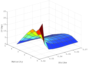
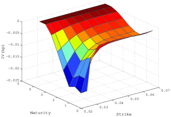
Figure 4.1. Difference in implied caplet volatility (in basis points) between the full SDE and the frozen drift prices (left), and the full SDE and the Picard approximation (right).

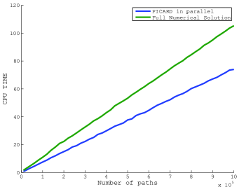
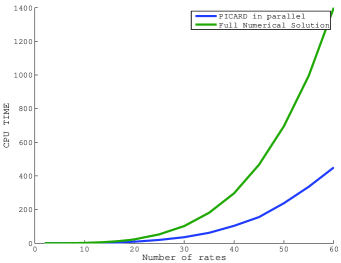
Figure 4.2. CPU time as function of the number of paths (left) and CPU time as a function of $N$, the number of rates (right).

In terms of computational time a large gain is realized when using the approximations in (3.2) and (3.2). In the example above the CPU time for the full numerical solution is 141 seconds but after applying the first order or second order drift approximation it drops to 0.9 and 1.2 respectively. Adding the Picard approximation to these three cases does not contribute to the computational speed unless parallelization is employed. On the left in figure 4.2, CPU time as function of the number of paths for the Picard approximation and the full numerical solution is plotted. Both use the second order drift approximation scheme in (3.2). The computations are done in Matlab running on an Intel i7 processor with the capability of running 8 processes simultaneously. Here we see the typical linear behavior as the number of paths are increased but it can be seen that the Picard approximation has a significantly lower slope. Furthermore, on the right when we plot CPU time as a function of rates one can see CPU time exponentially increasing, revealing that large gains in computational time are realizable when using the Picard approximation scheme and the drift expansion.

5. Conclusion

This paper derives a new approximation method for Monte Carlo derivative pricing in LIBOR models. It is generic and can be used for any semi-martingale driven model. It decouples the interdependence of the rates when moving them forward in time in a simulation, meaning that the computations can be parallelized in the maturity dimension. We have demonstrated both the accuracy and speed of the method in a numerical example.

References

- [\citeauthoryearAndersen and Brotherton-RatcliffeAndersen and Brotherton-Ratcliffe2005] Andersen, L. and R. Brotherton-Ratcliffe (2005). Extended LIBOR market models with stochastic volatility. J. Comput. Finance 9, 1–40.
- [\citeauthoryearBlackBlack1976] Black, F. (1976). The pricing of commodity contracts. J. Financ. Econ. 3, 167–179.
- [\citeauthoryearBrace, Dun, and BartonBrace et al.2001] Brace, A., T. Dun, and G. Barton (2001). Towards a central interest rate model. In E. Jouini, J. Cvitanić, and M. Musiela (Eds.), Option pricing, interest rates and risk management, pp. 278–313. Cambridge University Press.
- [\citeauthoryearBrace, Ga̧tarek, and MusielaBrace et al.1997] Brace, A., D. Ga̧tarek, and M. Musiela (1997). The market model of interest rate dynamics. Math. Finance 7, 127–155.
- [\citeauthoryearEberlein and ÖzkanEberlein and Özkan2005] Eberlein, E. and F. Özkan (2005). The Lévy LIBOR model. Finance Stoch. 9, 327–348.
- [\citeauthoryearGlassermanGlasserman2003] Glasserman, P. (2003). Monte Carlo methods in financial engineering. Springer-Verlag.
- [\citeauthoryearGlasserman and KouGlasserman and Kou2003] Glasserman, P. and S. G. Kou (2003). The term structure of simple forward rates with jump risk. Math. Finance 13, 383–410.
- [\citeauthoryearGlasserman and MerenerGlasserman and Merener2003a] Glasserman, P. and N. Merener (2003a). Cap and swaption approximations in LIBOR market models with jumps. J. Comput. Finance 7, 1–36.
- [\citeauthoryearGlasserman and MerenerGlasserman and Merener2003b] Glasserman, P. and N. Merener (2003b). Numerical solution of jump-diffusion LIBOR market models. Finance Stoch. 7, 1–27.
- [\citeauthoryearJamshidianJamshidian1999] Jamshidian, F. (1999). LIBOR market model with semimartingales. Working Paper, NetAnalytic Ltd.
- [\citeauthoryearJoshi and StaceyJoshi and Stacey2008] Joshi, M. and A. Stacey (2008). New and robust drift approximations for the LIBOR market model. Quant. Finance 8, 427–434.
- [\citeauthoryearKlugeKluge2005] Kluge, W. (2005). Time-inhomogeneous Lévy processes in interest rate and credit risk models. Ph. D. thesis, Univ. Freiburg.
- [\citeauthoryearMiltersen, Sandmann, and SondermannMiltersen et al.1997] Miltersen, K. R., K. Sandmann, and D. Sondermann (1997). Closed form solutions for term structure derivatives with log-normal interest rates. J. Finance 52, 409–430.
- [\citeauthoryearSandmann, Sondermann, and MiltersenSandmann et al.1995] Sandmann, K., D. Sondermann, and K. R. Miltersen (1995). Closed form term structure derivatives in a Heath–Jarrow–Morton model with log-normal annually compounded interest rates. In Proceedings of the Seventh Annual European Futures Research Symposium Bonn, pp. 145–165. Chicago Board of Trade.