Stability Approach to Regularization Selection (StARS) for High Dimensional Graphical Models

Abstract

A challenging problem in estimating high-dimensional graphical models is to choose the regularization parameter in a data-dependent way. The standard techniques include $K$-fold cross-validation ($K$-CV), Akaike information criterion (AIC), and Bayesian information criterion (BIC). Though these methods work well for low-dimensional problems, they are not suitable in high dimensional settings. In this paper, we present StARS: a new stability-based method for choosing the regularization parameter in high dimensional inference for undirected graphs. The method has a clear interpretation: we use the least amount of regularization that simultaneously makes a graph sparse and replicable under random sampling. This interpretation requires essentially no conditions. Under mild conditions, we show that StARS is partially sparsistent in terms of graph estimation: i.e. with high probability, all the true edges will be included in the selected model even when the graph size diverges with the sample size. Empirically, the performance of StARS is compared with the state-of-the-art model selection procedures, including $K$-CV, AIC, and BIC, on both synthetic data and a real microarray dataset. StARS outperforms all these competing procedures.

,  and

1 Introduction

Undirected graphical models have emerged as a useful tool because they allow for a stochastic description of complex associations in high-dimensional data. For example, biological processes in a cell lead to complex interactions among gene products. It is of interest to determine which features of the system are conditionally independent. Such problems require us to infer an undirected graph from i.i.d. observations. Each node in this graph corresponds to a random variable and the existence of an edge between a pair of nodes represent their conditional independence relationship.

Gaussian graphical models (Dempster, 1972; Whittaker, 1990; Edwards, 1995; Lauritzen, 1996) are by far the most popular approach for learning high dimensional undirected graph structures. Under the Gaussian assumption, the graph can be estimated using the sparsity pattern of the inverse covariance matrix. If two variables are conditionally independent, the corresponding element of the inverse covariance matrix is zero. In many applications, estimating the the inverse covariance matrix is statistically challenging because the number of features measured may be much larger than the number of collected samples. To handle this challenge, the graphical lasso or glasso (Friedman, Hastie and Tibshirani, 2007; Yuan and Lin, 2007; Banerjee, Ghaoui and d’Aspremont, 2008) is rapidly becoming a popular method for estimating sparse undirected graphs. To use this method, however, the user must specify a regularization parameter $\lambda$ that controls the sparsity of the graph. The choice of $\lambda$ is critical since different $\lambda$’s may lead to different scientific conclusions of the statistical inference. Other methods for estimating high dimensional graphs include (Meinshausen and Bühlmann, 2006; Peng et al., 2009; Liu, Lafferty and Wasserman, 2009). They also require the user to specify a regularization parameter.

The standard methods for choosing the regularization parameter are AIC (Akaike, 1973), BIC (Schwarz, 1978) and cross validation (Efron, 1982). Though these methods have good theoretical properties in low dimensions, they are not suitable for high dimensional problems. In regression, cross-validation has been shown to overfit the data (Wasserman and Roeder, 2009). Likewise, AIC and BIC tend to perform poorly when the dimension is large relative to the sample size. Our simulations confirm that these methods perform poorly when used with glasso.

A new approach to model selection, based on model stability, has recently generated some interest in the literature (Lange et al., 2004). The idea, as we develop it, is based on subsampling (Politis, Romano and Wolf, 1999) and builds on the approach of Meinshausen and Bühlmann (2010). We draw many random subsamples and construct a graph from each subsample (unlike $K$-fold cross-validation, these subsamples are overlapping). We choose the regularization parameter so that the obtained graph is sparse and there is not too much variability across subsamples. More precisely, we start with a large regularization which corresponds to an empty, and hence highly stable, graph. We gradually reduce the amount of regularization until there is a small but acceptable amount of variability of the graph across subsamples. In other words, we regularize to the point that we control the dissonance between graphs. The procedure is named StARS: Stability Approach to Regularization Selection. We study the performance of StARS by simulations and theoretical analysis in Sections 4 and 5. Although we focus here on graphical models, StARS is quite general and can be adapted to other settings including regression, classification, clustering, and dimensionality reduction.

In the context of clustering, results of stability methods have been mixed. Weaknesses of stability have been shown in (Ben-david, Luxburg and Pal, 2006). However, the approach was successful for density-based clustering (Rinaldo and Wasserman, 2009). For graph selection, Meinshausen and Bühlmann (2010) also used a stability criterion; however, their approach differs from StARS in its fundamental conception. They use subsampling to produce a new and more stable regularization path then select a regularization parameter from this newly created path, whereas we propose to use subsampling to directly select one regularization parameter from the original path. Our aim is to ensure that the selected graph is sparse, but inclusive, while they aim to control the familywise type I errors. As a consequence, their goal is contrary to ours: instead of selecting a larger graph that contains the true graph, they try to select a smaller graph that is contained in the true graph. As we will discuss in Section 3, in specific application domains like gene regulatory network analysis, our goal for graph selection is more natural.

In Section 2 we review the basic notion of estimating high dimensional undirected graphs; in Section 3 we develop StARS; in Section 4 we present a theoretical analysis of the proposed method; and in Section 5 we report experimental results on both simulated data and a gene microarray dataset, where the problem is to construct gene regulatory network based on natural variation of the expression levels of human genes.

2 Estimating a High-dimensional Undirected Graph

Let $X=\bigl{(}X(1),\ldots,X(p)\bigr{)}^{T}$ be a random vector with distribution $P$. The undirected graph $G=(V,E)$ associated with $P$ has vertices $V=\{X(1),\ldots,X(p)\}$ and a set of edges $E$ corresponding to pairs of vertices. In this paper, we also interchangeably use $E$ to denote the adjacency matrix of the graph $G$. The edge corresponding to $X(j)$ and $X(k)$ is absent if $X(j)$ and $X(k)$ are conditionally independent given the other coordinates of $X$. The graph estimation problem is to infer $E$ from i.i.d. observed data $X_{1},\ldots,X_{n}$ where $X_{i}=(X_{i}(1),\ldots,X_{i}(p))^{T}$.

Suppose now that $P$ is Gaussian with mean vector $\mu$ and covariance matrix $\Sigma$. Then the edge corresponding to $X(j)$ and $X(k)$ is absent if and only if $\Omega_{jk}=0$ where $\Omega=\Sigma^{-1}$. Hence, to estimate the graph we only need to estimate the sparsity pattern of $\Omega$. When $p$ could diverge with $n$, estimating $\Omega$ is difficult. A popular approach is the graphical lasso or glasso (Friedman, Hastie and Tibshirani, 2007; Yuan and Lin, 2007; Banerjee, Ghaoui and d’Aspremont, 2008). Using glasso, we estimate $\Omega$ as follows: Ignoring constants, the log-likelihood (after maximizing over $\mu$) can be written as

$$\ell(\Omega)=\log|\Omega|-\text{trace}\bigl{(}\widehat{\Sigma}\Omega\bigr{)}$$

where $\widehat{\Sigma}$ is the sample covariance matrix. With a positive regularization parameter $\lambda$, the glasso estimator $\widehat{\Omega}(\lambda)$ is obtained by minimizing the regularized negative log-likelihood

$$\widehat{\Omega}(\lambda)=\mathop{\text{\rm arg\,min}}_{\Omega\succ 0}\Bigl{\{}-\ell(\Omega)+\lambda||\Omega||_{1}\Bigr{\}}$$ (2.1)

where $||\Omega||_{1}=\sum_{j,k}|\Omega_{jk}|$ is the elementwise $\ell_{1}$-norm of $\Omega$. The estimated graph $\widehat{G}(\lambda)=(V,\widehat{E}(\lambda))$ is then easily obtained from $\widehat{\Omega}(\lambda)$: for $i\neq j$, an edge $(i,j)\in\widehat{E}(\lambda)$ if and only if the corresponding entry in $\widehat{\Omega}(\lambda)$ is nonzero. Friedman, Hastie and Tibshirani (2007) give a fast algorithm for calculating $\widehat{\Omega}(\lambda)$ over a grid of $\lambda$s ranging from small to large. By taking advantage of the fact that the objective function in (2.1) is convex, their algorithm iteratively estimates a single row (and column) of $\Omega$ in each iteration by solving a lasso regression (Tibshirani, 1996). The resulting regularization path $\widehat{\Omega}(\lambda)$ for all $\lambda$s has been shown to have excellent theoretical properties (Rothman et al., 2008; Ravikumar et al., 2009). For example, Ravikumar et al. (2009) show that, if the regularization parameter $\lambda$ satisfies a certain rate, the corresponding estimator $\widehat{\Omega}(\lambda)$ could recover the true graph with high probability. However, these types of results are either asymptotic or non-asymptotic but with very large constants. They are not practical enough to guide the choice of the regularization parameter $\lambda$ in finite-sample settings.

3 Regularization Selection

In Equation (2.1), the choice of $\lambda$ is critical because $\lambda$ controls the sparsity level of $\widehat{G}(\lambda)$. Larger values of $\lambda$ tend to yield sparser graphs and smaller values of $\lambda$ yield denser graphs. It is convenient to define $\Lambda=1/\lambda$ so that small $\Lambda$ corresponds to a more sparse graph. In particular, $\Lambda=0$ corresponds to the empty graph with no edges. Given a grid of regularization parameters $\mathcal{G}_{n}=\{\Lambda_{1},\ldots,\Lambda_{K}\}$, our goal of graph regularization parameter selection is to choose one $\widehat{\Lambda}\in\mathcal{G}_{n}$, such that the true graph $E$ is contained in $\widehat{E}(\widehat{\Lambda})$ with high probability. In other words, we want to “overselect” instead of “underselect”. Such a choice is motivated by application problems like gene regulatory networks reconstruction, in which we aim to study the interactions of many genes. For these types of studies, we tolerant some false positives but not false negatives. Specifically, it is acceptable that an edge presents but the two genes corresponding to this edge do not really interact with each other. Such false positives can generally be screened out by more fine-tuned downstream biological experiments. However, if one important interaction edge is omitted at the beginning, it’s very difficult for us to re-discovery it by follow-up analysis. There is also a tradeoff: we want to select a denser graph which contains the true graph with high probability. At the same time, we want the graph to be as sparse as possible so that important information will not be buried by massive false positives. Based on this rationale, an “underselect” method, like the approach of Meinshausen and Bühlmann (2010), does not really fit our goal. In the following, we start with an overview of several state-of-the-art regularization parameter selection methods for graphs. We then introduce our new StARS approach.

3.1 Existing Methods

The regularization parameter is often chosen using AIC or BIC. Let $\widehat{\Omega}(\Lambda)$ denote the estimator corresponding to $\Lambda$. Let $d(\Lambda)$ denote the degree of freedom (or the effective number of free parameters) of the corresponding Gaussian model. AIC chooses $\Lambda$ as

$$\mathrm{(AIC)}\quad\widehat{\Lambda}=\mathop{\text{\rm arg\,min}}_{\Lambda\in\mathcal{G}_{n}}\bigl{\{}-2\ell\bigl{(}\widehat{\Omega}(\Lambda)\bigr{)}+2d(\Lambda)\bigr{\}},$$ (3.1)

and BIC chooses $\Lambda$ as

$$\mathrm{(BIC)}\quad\widehat{\Lambda}=\mathop{\text{\rm arg\,min}}_{\Lambda\in\mathcal{G}_{n}}\bigl{\{}-2\ell\bigl{(}\widehat{\Omega}(\Lambda)\bigr{)}+d(\Lambda)\cdot\log n\bigr{\}}.$$ (3.2)

The usual theoretical justification for these methods assumes that the dimension $p$ is fixed as $n$ increases; however, in the case where $p>n$ this justification is not applicable. In fact, it’s even not straightforward how to estimate the degree of freedom $d(\Lambda)$ when $p$ is larger than $n$ . A common practice is to calculate $d(\Lambda)$ as $d(\Lambda)=m(\Lambda)(m(\Lambda)-1)/2+p$ where $m(\Lambda)$ denotes the number of nonzero elements of $\widehat{\Omega}(\Lambda)$. As we will see in our experiments, AIC and BIC tend to select overly dense graphs in high dimensions.

Another popular method is $K$-fold cross-validation ($K$-CV). For this procedure the data is partitioned into $K$ subsets. Of the $K$ subsets one is retained as the validation data, and the remaining $K-1$ ones are used as training data. For each $\Lambda\in\mathcal{G}_{n}$, we estimate a graph on the $K-1$ training sets and evaluate the negative log-likelihood on the retained validation set. The results are averaged over all $K$ folds to obtain a single CV score. We then choose $\Lambda$ to minimize the CV score over he whole grid $\mathcal{G}_{n}$. In regression, cross-validation has been shown to overfit (Wasserman and Roeder, 2009). Our experiments will confirm this is true for graph estimation as well.

3.2 StARS: Stability Approach to Regularization Selection

The StARS approach is to choose $\Lambda$ based on stability. When $\Lambda$ is 0, the graph is empty and two datasets from $P$ would both yield the same graph. As we increase $\Lambda$, the variability of the graph increases and hence the stability decreases. We increase $\Lambda$ just until the point where the graph becomes variable as measured by the stability. StARS leads to a concrete rule for choosing $\Lambda$.

Let $b=b(n)$ be such that $1<b(n)<n$. We draw $N$ random subsamples $S_{1},\ldots,S_{N}$ from $X_{1},\ldots,X_{n}$, each of size $b$. There are $\binom{n}{b}$ such subsamples. Theoretically one uses all $\binom{n}{b}$ subsamples. However, Politis, Romano and Wolf (1999) show that it suffices in practice to choose a large number $N$ of subsamples at random. Note that, unlike bootstrapping (Efron, 1982), each subsample is drawn without replacement. For each $\Lambda\in\mathcal{G}_{n}$, we construct a graph using the glasso for each subsample. This results in $N$ estimated edge matrices $\widehat{E}^{b}_{1}(\Lambda),\ldots,\widehat{E}^{b}_{N}(\Lambda)$. Focus for now on one edge $(s,t)$ and one value of $\Lambda$. Let $\psi^{\Lambda}(\cdot)$ denote the glasso algorithm with the regularization parameter $\Lambda$. For any subsample $S_{j}$ let $\psi_{st}^{\Lambda}(S_{j})=1$ if the algorithm puts an edge and $\psi^{\Lambda}_{st}(S_{j})=0$ if the algorithm does not put an edge between $(s,t)$. Define

$$\theta^{b}_{st}(\Lambda)=\mathbb{P}(\psi^{\Lambda}_{st}(X_{1},\ldots,X_{b})=1).$$

To estimate $\theta^{b}_{st}(\Lambda)$, we use a U-statistic of order $b$, namely,

$$\widehat{\theta}^{b}_{st}(\Lambda)=\frac{1}{N}\sum_{j=1}^{N}\psi^{\Lambda}_{st}(S_{j}).$$

Now define the parameter $\xi^{b}_{st}(\Lambda)=2\theta^{b}_{st}(\Lambda)(1-\theta^{b}_{st}(\Lambda))$ and let $\widehat{\xi}^{b}_{st}(\Lambda)=2\widehat{\theta}^{b}_{st}(\Lambda)(1-\widehat{\theta}^{b}_{st}(\Lambda))$ be its estimate. Then $\xi^{b}_{st}(\Lambda)$, in addition to being twice the variance of the Bernoulli indicator of the edge $(s,t)$, has the following nice interpretation: For each pair of graphs, we can ask how often they disagree on the presence of the edge: $\xi^{b}_{st}(\Lambda)$ is the fraction of times they disagree. For $\Lambda\in\mathcal{G}_{n}$, we regard $\xi^{b}_{st}(\Lambda)$ as a measure of instability of the edge across subsamples, with $0\leq\xi^{b}_{st}(\Lambda)\leq 1/2$.

Define the total instability by averaging over all edges:

$$\widehat{D}_{b}(\Lambda)=\frac{\sum_{s<t}\widehat{\xi}^{b}_{st}}{\binom{p}{2}}.$$

Clearly on the boundary $\widehat{D}_{b}(0)=0$, and $\widehat{D}_{b}(\Lambda)$ generally will increase as $\Lambda$ increases. However, when $\Lambda$ gets very large, all the graphs will become dense and $\widehat{D}_{b}(\Lambda)$ will begin to decrease. Subsample stability for large $\Lambda$ is essentially an artifact. We are interested in stability for sparse graphs not dense graphs. For this reason we monotonize $\widehat{D}_{b}(\Lambda)$ by defining $\overline{D}_{b}(\Lambda)=\sup_{0\leq t\leq\Lambda}\widehat{D}_{b}(t)$. Finally, our StARS approach chooses $\Lambda$ by defining $\widehat{\Lambda}_{\rm s}=\sup\Bigl{\{}\Lambda:\ \overline{D}_{b}(\Lambda)\leq\beta\Bigr{\}}$ for a specified cut point value $\beta$.

It may seem that we have merely replaced the problem of choosing $\Lambda$ with the problem of choosing $\beta$, but $\beta$ is an interpretable quantity and we always set a default value $\beta=0.05$. One thing to note is that all quantities $\widehat{E},\widehat{\theta},\widehat{\xi},\widehat{D}$ depend on the subsampling block size $b$. Since StARS is based on subsampling, the effective sample size for estimating the selected graph is $b$ instead of $n$. Compared with methods like BIC and AIC which fully utilize all $n$ data points. StARS has some efficiency loss in low dimensions. However, in high dimensional settings, the gain of StARS on better graph selection significantly dominate this efficiency loss. This fact is confirmed by our experiments.

4 Theoretical Properties

The StARS procedure is quite general and can be applied with any graph estimation algorithms. Here, we provide its theoretical properties. We start with a key theorem which establishes the rates of convergence of the estimated stability quantities to their population means. We then discuss the implication of this theorem on general gaph regularization selection problems.

Let $\Lambda$ be an element in the grid ${\cal G}_{n}=\{\Lambda_{1},\ldots,\Lambda_{K}\}$ where $K$ is a polynomial of $n$. We denote $D_{b}(\Lambda)=\mathbb{E}(\widehat{D}_{b}(\Lambda))$. The quantity $\widehat{\xi}^{b}_{st}(\Lambda)$ is an estimate of $\xi^{b}_{st}(\Lambda)$ and $\widehat{D}_{b}(\Lambda)$ is an estimate of ${D}_{b}(\Lambda)$. Standard $U$-statistic theory guarantees that these estimates have good uniform convergence properties to their population quantities:

Theorem 4.1.

(Uniform Concentration) The following statements hold with no assumptions on $P$. For any $\delta\in(0,1)$, with probability at least $1-\delta$, we have

$$\forall\Lambda\in\mathcal{G}_{n},~{}\max_{s<t}|\widehat{\xi}^{b}_{st}(\Lambda)-\xi^{b}_{st}(\Lambda)|\leq\sqrt{\frac{18b\left(2\log p+\log(2/\delta)\right)}{n}},$$ (4.1)

$$\max_{\Lambda\in{\cal G}_{n}}|\widehat{D}_{b}(\Lambda)-D_{b}(\Lambda)|\leq\sqrt{\frac{18b\left(\log K+4\log p+\log\left(1/\delta\right)\right)}{{n}}}.$$ (4.2)

Proof.

Note that $\widehat{\theta}^{b}_{st}(\Lambda)$ is a $U$-statistic of order $b$. Hence, by Hoeffding’s inequality for $U$-statistics (Serfling, 1980), we have, for any $\epsilon>0$,

$$\mathbb{P}(|\widehat{\theta}^{b}_{st}(\Lambda)-\theta^{b}_{st}(\Lambda)|>\epsilon)\leq 2\exp\left({-2n\epsilon^{2}/b}\right).$$ (4.3)

Now $\widehat{\xi}^{b}_{st}(\Lambda)$ is just a function of the $U$-statistic $\widehat{\theta}^{b}_{st}(\Lambda)$. Note that

$$|\widehat{\xi}^{b}_{st}(\Lambda)-\xi^{b}_{st}(\Lambda)| = 2|\widehat{\theta}^{b}_{st}(\Lambda)(1-\widehat{\theta}^{b}_{st}(\Lambda))-\theta^{b}_{st}(\Lambda)(1-\theta^{b}_{st}(\Lambda))|$$ (4.4)

$$= 2|\widehat{\theta}^{b}_{st}(\Lambda)-\bigl{(}\widehat{\theta}^{b}_{st}(\Lambda)\bigr{)}^{2}-\theta^{b}_{st}(\Lambda)+\bigl{(}\theta^{b}_{st}(\Lambda)\bigr{)}^{2}|$$ (4.5)

$$\leq 2|\widehat{\theta}^{b}_{st}(\Lambda)-\theta^{b}_{st}(\Lambda)|+2|\bigl{(}\widehat{\theta}^{b}_{st}(\Lambda)\bigr{)}^{2}-\bigl{(}\theta^{b}_{st}(\Lambda)\bigr{)}^{2}|$$ (4.6)

$$\leq 2|\widehat{\theta}^{b}_{st}(\Lambda)-\theta^{b}_{st}(\Lambda)|+2|(\widehat{\theta}^{b}_{st}(\Lambda)-\theta^{b}_{st}(\Lambda))(\widehat{\theta}^{b}_{st}(\Lambda)+\theta^{b}_{st}(\Lambda))|$$ (4.7)

$$\leq 2|\widehat{\theta}^{b}_{st}(\Lambda)-\theta^{b}_{st}(\Lambda)|+4|\widehat{\theta}^{b}_{st}(\Lambda)-\theta^{b}_{st}(\Lambda)|$$ (4.8)

$$= 6|\widehat{\theta}^{b}_{st}(\Lambda)-\theta^{b}_{st}(\Lambda)|,$$ (4.9)

we have $|\widehat{\xi}^{b}_{st}(\Lambda)-\xi^{b}_{st}(\Lambda)|\leq 6|\widehat{\theta}^{b}_{st}(\Lambda)-\theta^{b}_{st}(\Lambda)|$. Using (4.3) and the union bound over all the edges, we obtain: for each $\Lambda\in\mathcal{G}_{n}$,

$$\mathbb{P}(\max_{s<t}|\widehat{\xi}^{b}_{st}(\Lambda)-\xi^{b}_{st}(\Lambda)|>6\epsilon)\leq 2p^{2}\exp\left({-2n\epsilon^{2}/b}\right).$$ (4.10)

Using two union bound arguments over the $K$ values of $\Lambda$ and all the $p(p-1)/2$ edges, we have:

$$\mathbb{P}\left(\max_{\Lambda\in{\cal G}_{n}}|\widehat{D}_{b}(\Lambda)-D_{b}(\Lambda)|\geq\epsilon\right) \leq |\mathcal{G}_{n}|\cdot\frac{p(p-1)}{2}\cdot\mathbb{P}(\max_{s<t}|\widehat{\xi}^{b}_{st}(\Lambda)-\xi^{b}_{st}(\Lambda)|>\epsilon)$$ (4.11)

$$\leq K\cdot p^{4}\cdot\exp\left(-{n\epsilon^{2}}/{(18b)}\right).$$ (4.12)

Equations (4.1) and (4.2) follow directly from (4.10) and the above exponential probability inequality. ∎

Theorem 4.1 allows us to explicitly characterize the high-dimensional scaling of the sample size $n$, dimensionality $p$, subsampling block size $b$, and the grid size $K$. More specifically, we get

$$\frac{n}{b\log\bigl{(}np^{4}K\bigr{)}}\rightarrow\infty\implies\max_{\Lambda\in{\cal G}_{n}}|\widehat{D}_{b}(\Lambda)-D_{b}(\Lambda)|\stackrel{{\scriptstyle P}}{{\to}}0$$ (4.13)

by setting $\delta=1/n$ in Equation (4.2). From (4.13), let $c_{1},c_{2}$ be arbitrary positive constants, if $b=c_{1}\sqrt{n}$, $K=n^{c_{2}}$, and $p\leq\exp\left({n^{\gamma}}\right)$ for some $\gamma<1/2$, the estimated total stability $\widehat{D}_{b}(\Lambda)$ still converges to its mean $D_{b}(\Lambda)$ uniformly over the whole grid $\mathcal{G}_{n}$.

We now discuss the implication of Theorem 4.1 to graph regularization selection problems. Due to the generality of StARS, we provide theoretical justifications for a whole family of graph estimation procedures satisfying certain conditions. Let $\psi$ be a graph estimation procedure. We denote $\widehat{E}^{b}(\Lambda)$ as the estimated edge set using the regularization parameter $\Lambda$ by applying $\psi$ on a subsampled dataset with block size $b$. To establish graph selection result, we start with two technical assumptions:

• $\exists\Lambda_{\rm o}\in\mathcal{G}_{n}$, such that $\max_{\Lambda\leq\Lambda_{\rm o}\wedge\Lambda\in\mathcal{G}_{n}}D_{b}(\Lambda)\leq{\beta}/{2}$ for large enough $n$.

• For any $\Lambda\in\mathcal{G}_{n}$ and $\Lambda\geq\Lambda_{\rm o}$, $\mathbb{P}\bigl{(}E\subset\widehat{E}^{b}(\Lambda)\bigr{)}\rightarrow 1$ as $n\rightarrow\infty$.

Note that $\Lambda_{\rm o}$ here depends on the sample size $n$ and does not have to be unique. To understand the above conditions, (A1) assumes that there exists a threshold $\Lambda_{\rm o}\in\mathcal{G}_{n}$, such that the population quantity $D_{b}(\Lambda)$ is small for all $\Lambda\leq\Lambda_{\rm o}$. (A2) requires that all estimated graphs using regularization parameters $\Lambda\geq\Lambda_{\rm o}$ contain the true graph with high probability. Both assumptions are mild and should be satisfied by most graph estimation algorithm with reasonable behaviors. There is a tradeoff on the design of the subsampling block size $b$ . To make (A2) hold, we require $b$ to be large. However, to make $\widehat{D}_{b}(\Lambda)$ concentrate to $D_{b}(\Lambda)$ fast, we require $b$ to be small. Our suggested value is $b=\lfloor 10\sqrt{n}\rfloor$, which balances both the theoretical and empirical performance well. The next theorem provides the graph selection performance of StARS:

Theorem 4.2.

(Partial Sparsistency): Let $\psi$ to be a graph estimation algorithm. We assume (A1) and (A2) hold for $\psi$ using $b=\lfloor 10\sqrt{n}\rfloor$ and $|\mathcal{G}_{n}|=K=n^{c_{1}}$ for some constant $c_{1}>0$. Let $\widehat{\Lambda}_{\rm s}\in\mathcal{G}_{n}$ be the selected regularization parameter using the StARS procedure with a constant cutting point $\beta$. Then, if $p\leq\exp\left({n^{\gamma}}\right)$ for some $\gamma<1/2$, we have

$$\mathbb{P}\bigl{(}E\subset\widehat{E}^{b}(\widehat{\Lambda}_{\rm s})\bigr{)}\rightarrow 1~{}~{}\text{as}~{}~{}n\rightarrow\infty.$$ (4.14)

Proof.

We define $\mathcal{A}_{n}$ to be the event that $\max_{\Lambda\in{\cal G}_{n}}|\widehat{D}_{b}(\Lambda)-D_{b}(\Lambda)|\leq\beta/2$. The scaling of $n,K,b,p$ in the theorem satisfies the L.H.S. of (4.13), which implies that $\mathbb{P}(\mathcal{A}_{n})\rightarrow 1$ as $n\rightarrow\infty$.

Using (A1), we know that, on $\mathcal{A}_{n}$,

$$\max_{\Lambda\leq\Lambda_{\rm o}\wedge\Lambda\in\mathcal{G}_{n}}\widehat{D}_{b}(\Lambda)\leq\max_{\Lambda\in{\cal G}_{n}}|\widehat{D}_{b}(\Lambda)-D_{b}(\Lambda)|+\max_{\Lambda\leq\Lambda_{\rm o}\wedge\Lambda\in\mathcal{G}_{n}}D_{b}(\Lambda)\leq\beta.$$ (4.15)

This implies that, on $\mathcal{A}_{n}$, $\widehat{\Lambda}_{\rm s}\geq{\Lambda}_{\rm o}$. The result follows by applying (A2) and a union bound. ∎

5 Experimental Results

We now provide empirical evidence to illustrate the usefulness of StARS and compare it with several state-of-the-art competitors, including $10$-fold cross-validation ($K$-CV), BIC, and AIC. For StARS we always use subsampling block size $b(n)=\lfloor 10\cdot\sqrt{n}]$ and set the cut point $\beta=0.05$. We first quantitatively evaluate these methods on two types of synthetic datasets, where the true graphs are known. We then illustrate StARS on a microarray dataset that records the gene expression levels from immortalized B cells of human subjects. On all high dimensional synthetic datasets, StARS significantly outperforms its competitors. On the microarray dataset, StARS obtains a remarkably simple graph while all competing methods select what appear to be overly dense graphs.

5.1 Synthetic Data

To quantitatively evaluate the graph estimation performance, we adapt the criteria including precision, recall, and $F_{1}$-score from the information retrieval literature. Let $G=(V,E)$ be a $p$-dimensional graph and let $\widehat{G}=(V,\widehat{E})$ be an estimated graph. We define

$$\text{precision}=\frac{|\widehat{E}\cap E|}{|\widehat{E}|},~{}~{}\text{recall}=\frac{|\widehat{E}\cap E|}{|E|},~{}~{}F_{1}\text{-score}=2\cdot\frac{\text{precision}\cdot\text{recall}}{\text{precision}+\text{recall}}.$$ (5.1)

In other words, Precision is the number of correctly estimated edges divided by the total number of edges in the estimated graph; recall is the number of correctly estimated edges divided by the total number of edges in the true graph; the $F_{1}$-score can be viewed as a weighted average of the precision and recall, where an $F_{1}$-score reaches its best value at 1 and worst score at 0. On the synthetic data where we know the true graphs, we also compare the previous methods with an oracle procedure which selects the optimal regularization parameter by minimizing the total number of different edges between the estimated and true graphs along the full regularization path. Since this oracle procedure requires the knowledge of the truth graph, it is not a practical method. We only present it here to calibrate the inherent challenge of each simulated scenario. To make the comparison fair, once the regularization parameters are selected, we estimate the oracle and StARS graphs only based on a subsampled dataset with size

$$b(n)=\lfloor 10\sqrt{n}\rfloor.$$

In contrast, the $K$-CV, BIC, and AIC graphs are estimated using the full dataset. More details about this issue were discussed in Section 3.

We generate data from sparse Gaussian graphs, neighborhood graphs and hub graphs, which mimic characteristics of real-wolrd biological networks. The mean is set to be zero and the covariance matrix $\Sigma=\Omega^{-1}$. For both graphs, the diagonal elements of $\Omega$ are set to be one. More specifically:

1. Neighborhood graph: We first uniformly sample $y_{1},\ldots,y_{n}$ from a unit square. We then set $\Omega_{ij}=\Omega_{ji}=\rho$ with probability $\left(\sqrt{2\pi}\right)^{-1}\exp\left(-4\|y_{i}-y_{j}\|^{2}\right)$. All the rest $\Omega_{ij}$ are set to be zero. The number of nonzero off-diagonal elements of each row or column is restricted to be smaller than $\lfloor 1/\rho\rfloor$. In this paper, $\rho$ is set to be 0.245.

2. Hub graph: The rows/columns are partitioned into $J$ equally-sized disjoint groups: $V_{1}\cup V_{2}\ldots\cup V_{J}=\{1,\ldots,p\}$, each group is associated with a “pivotal” row $k$. Let $|V_{1}|=s$. We set $\Omega_{ik}=\Omega_{ki}=\rho$ for $i\in V_{k}$ and $\Omega_{ik}=\Omega_{ki}=0$ otherwise. In our experiment, $J=\lfloor p/s\rfloor$, $k=1,s+1,2s+1,\ldots$, and we always set $\rho=1/(s+1)$ with $s=20$.

We generate synthetic datasets in both low-dimensional ($n=800,p=40$) and high-dimensional ($n=400,p=100$) settings. Table 1 provides comparisons of all methods, where we repeat the experiments 100 times and report the averaged precision, recall, $F_{1}$-score with their standard errors.

Table 1: Quantitative comparison of different methods on the datasets from the neighborhood and hub graphs.

Neighborhood graph: n =800, p=40    Neighborhood graph: n=400, p =100
$\displaystyle\mathbf{Methods}$	Precision	Recall	$F_{1}\text{-score}$	Precision	Recall	$F_{1}\text{-score}$
Oracle	$0.9222\ (0.05)$	$0.9070\ (0.07)$	$0.9119\ (0.04)$	$\displaystyle 0.7473\ (0.09)$	$0.8001\ (0.06)$	$0.7672\ (0.07)$
StARS	$0.7204\ (0.08)$	$0.9530\ (0.05)$	$0.8171\ (0.05)$	$\displaystyle 0.6366\ (0.07)$	$0.8718\ (0.06)$	$0.7352\ (0.07)$
K-CV	$0.1394\ (0.02)$	$1.0000\ (0.00)$	$0.2440\ (0.04)$	$\displaystyle 0.1383\ (0.01)$	$1.0000\ (0.00)$	$0.2428\ (0.01)$
BIC	$0.9738\ (0.03)$	$0.9948\ (0.02)$	$0.9839\ (0.01)$	$\displaystyle 0.1796\ (0.11)$	$1.0000\ (0.00)$	$0.2933\ (0.13)$
AIC	$0.8696\ (0.11)$	$0.9996\ (0.01)$	$0.9236\ (0.07)$	$\displaystyle 0.1279\ (0.00)$	$1.0000\ (0.00)$	$0.2268\ (0.01)$

Hub graph: n =800, p=40    Hub graph: n=400, p =100
$\displaystyle\mathbf{Methods}$	Precision	Recall	$F_{1}\text{-score}$	Precision	Recall	$F_{1}\text{-score}$
Oracle	$0.9793\ (0.01)$	$1.0000\ (0.00)$	$0.9895\ (0.01)$	$\displaystyle 0.8976\ (0.02)$	$1.0000\ (0.00)$	$0.9459\ (0.01)$
StARS	$0.4377\ (0.02)$	$1.0000\ (0.00)$	$0.6086\ (0.02)$	$\displaystyle 0.4572\ (0.01)$	$1.0000\ (0.00)$	$0.6274\ (0.01)$
K-CV	$0.2383\ (0.09)$	$1.0000\ (0.00)$	$0.3769\ (0.01)$	$\displaystyle 0.1574\ (0.01)$	$1.0000\ (0.00)$	$0.2719\ (0.00)$
BIC	$0.4879\ (0.05)$	$1.0000\ (0.00)$	$0.6542\ (0.05)$	$\displaystyle 0.2155\ (0.00)$	$1.0000\ (0.00)$	$0.3545\ (0.01)$
AIC	$0.2522\ (0.09)$	$1.0000\ (0.00)$	$0.3951\ (0.00)$	$\displaystyle 0.1676\ (0.00)$	$1.0000\ (0.00)$	$0.2871\ (0.00)$

For low-dimensional settings where $n\gg p$, the BIC criterion is very competitive and performs the best among all the methods. In high dimensional settings, however, StARS clearly outperforms all the competing methods for both neighborhood and hub graphs. This is consistent with our theory. At first sight, it might be surprising that for data from low-dimensional neighborhood graphs, BIC and AIC even outperform the oracle procedure! This is due to the fact that both BIC and AIC graphs are estimated using all the $n=800$ data points, while the oracle graph is estimated using only the subsampled dataset with size $b(n)=\lfloor 10\cdot\sqrt{n}\rfloor=282$. Direct usage of the full sample is an advantage of model selection methods that take the general form of BIC and AIC. In high dimensions, however, we see that even with this advantage, StARS clearly outperforms BIC and AIC. The estimated graphs for different methods in the setting $n=400,p=100$ are provided in Figures 1 and 2, from which we see that the StARS graph is almost as good as the oracle, while the $K$-CV, BIC, and AIC graphs are overly too dense.

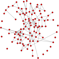
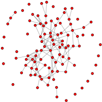
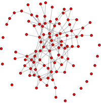
(a) True graph	(b) Oracle graph	(c) StARS graph
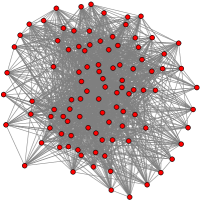
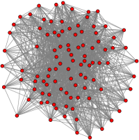
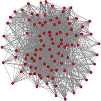
(d) $K$-CV graph	(e) BIC graph	(f) AIC graph

Figure 1: Comparison of different methods on the data from the neighborhood graphs ($n=400,p=100$).

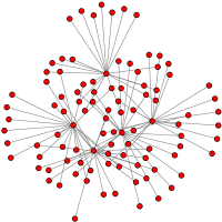
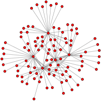
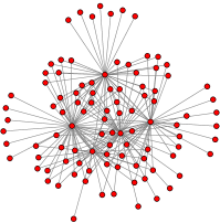
(a) True graph	(b) Oracle graph	(c) StARS graph
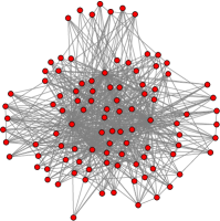
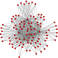
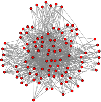
(d) $K$-CV graph	(e) BIC graph	(f) AIC graph

Figure 2: Comparison of different methods on the data from the hub graphs ($n=400,p=100$).

5.2 Microarray Data

We apply StARS to a dataset based on Affymetrix GeneChip microarrays for the gene expression levels from immortalized B cells of human subjects. The sample size is $n=294$. The expression levels for each array are pre-processed by log-transformation and standardization as in (Nayak et al., 2009). Using a previously estimated sub-pathway subset containing 324 genes (Liu et al., 2010), we study the estimated graphs obtained from each method under investigation. The StARS and BIC graphs are provided in Figure 3. We see that the StARS graph is remarkably simple and informative, exhibiting some cliques and hub genes. In contrast, the BIC graph is very dense and possible useful association information is buried in the large number of estimated edges. The selected graphs using AIC and $K$-CV are even more dense than the BIC graph and is omitted here. A full treatment of the biological implication of these two graphs validated by enrichment analysis will be left as a future study.

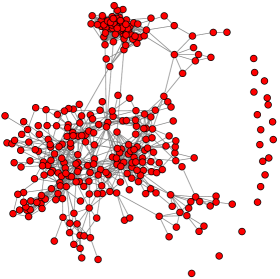
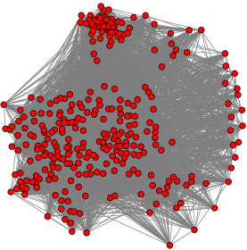
(a) StARS graph	(b) BIC graph

Figure 3: Microarray data example. The StARS graph is more informative graph than the BIC graph.

6 Conclusions

The problem of estimating structure in high dimensions is very challenging. Casting the problem in the context of a regularized optimization has led to some success, but the choice of the regularization parameter is critical. We present a new method, StARS, for choosing this parameter in high dimensional inference for undirected graphs. Like Meinshausen and Bühlmann’s stability selection approach (Meinshausen and Bühlmann, 2010), our method makes use of subsampling, but it differs substantially from their approach in both implementation and goals. For graphical models, we choose the regularization parameter directly based on the edge stability. Under mild conditions, StARS is partially sparsistent. However, even without these conditions, StARS has a simple interpretation: we use the least amount of regularization that simultaneously makes a graph sparse and replicable under random sampling.

Empirically, we show that StARS works significantly better than existing techniques on both synthetic and microarray datasets. Although we focus here on graphical models, our new method is generally applicable to many problems that involve estimating structure, including regression, classification, density estimation, clustering, and dimensionality reduction.

References

- Akaike (1973) {barticle}[author] \bauthor\bsnmAkaike, \bfnmHirotsugu\binitsH. (\byear1973). \btitleInformation theory and an extension of the maximum likelihood principle. \bjournalSecond International Symposium on Information Theory \banumber2 \bpages267-281. \endbibitem
- Banerjee, Ghaoui and d’Aspremont (2008) {barticle}[author] \bauthor\bsnmBanerjee, \bfnmOnureena\binitsO., \bauthor\bsnmGhaoui, \bfnmLaurent El\binitsL. E. and \bauthor\bsnmd’Aspremont, \bfnmAlexandre\binitsA. (\byear2008). \btitleModel selection through sparse maximum likelihood estimation. \bjournalJournal of Machine Learning Research \bvolume9 \bpages485–516. \endbibitem
- Ben-david, Luxburg and Pal (2006) {binproceedings}[author] \bauthor\bsnmBen-david, \bfnmShai\binitsS., \bauthor\bsnmLuxburg, \bfnmUlrike Von\binitsU. V. and \bauthor\bsnmPal, \bfnmDavid\binitsD. (\byear2006). \btitleA sober look at clustering stability. In \bbooktitleProceedings of the Conference of Learning Theory \bpages5–19. \bpublisherSpringer. \endbibitem
- Dempster (1972) {barticle}[author] \bauthor\bsnmDempster, \bfnmArthur P.\binitsA. P. (\byear1972). \btitleCovariance Selection. \bjournalBiometrics \bvolume28 \bpages157-175. \endbibitem
- Edwards (1995) {bbook}[author] \bauthor\bsnmEdwards, \bfnmDavid\binitsD. (\byear1995). \btitleIntroduction to graphical modelling. \bpublisherSpringer-Verlag Inc. \endbibitem
- Efron (1982) {bbook}[author] \bauthor\bsnmEfron, \bfnmBradley\binitsB. (\byear1982). \btitleThe jackknife, the bootstrap and other resampling plans. \bpublisherSIAM [Society for Industrial and Applied Mathematics]. \endbibitem
- Friedman, Hastie and Tibshirani (2007) {barticle}[author] \bauthor\bsnmFriedman, \bfnmJerome H.\binitsJ. H., \bauthor\bsnmHastie, \bfnmTrevor\binitsT. and \bauthor\bsnmTibshirani, \bfnmRobert\binitsR. (\byear2007). \btitleSparse inverse covariance estimation with the graphical lasso. \bjournalBiostatistics \bvolume9 \bpages432–441. \endbibitem
- Lange et al. (2004) {barticle}[author] \bauthor\bsnmLange, \bfnmTilman\binitsT., \bauthor\bsnmRoth, \bfnmVolker\binitsV., \bauthor\bsnmBraun, \bfnmMikio L.\binitsM. L. and \bauthor\bsnmBuhmann, \bfnmJoachim M.\binitsJ. M. (\byear2004). \btitleStability-Based Validation of Clustering Solutions. \bjournalNeural Computation \bvolume16 \bpages1299-1323. \endbibitem
- Lauritzen (1996) {bbook}[author] \bauthor\bsnmLauritzen, \bfnmSteffen L.\binitsS. L. (\byear1996). \btitleGraphical Models. \bpublisherOxford University Press. \endbibitem
- Liu, Lafferty and Wasserman (2009) {barticle}[author] \bauthor\bsnmLiu, \bfnmHan\binitsH., \bauthor\bsnmLafferty, \bfnmJohn\binitsJ. and \bauthor\bsnmWasserman, \bfnmLarry\binitsL. (\byear2009). \btitleThe Nonparanormal: Semiparametric Estimation of High Dimensional Undirected Graphs. \bjournalJournal of Machine Learning Research \bvolume10 \bpages2295-2328. \endbibitem
- Liu et al. (2010) {barticle}[author] \bauthor\bsnmLiu, \bfnmHan\binitsH., \bauthor\bsnmXu, \bfnmMin\binitsM., \bauthor\bsnmGu, \bfnmHaijie\binitsH., \bauthor\bsnmGupta, \bfnmAnupam\binitsA., \bauthor\bsnmLafferty, \bfnmJohn\binitsJ. and \bauthor\bsnmWasserman, \bfnmLarry\binitsL. (\byear2010). \btitleForest Density Estimation. \bjournalarXiv/1001.1557. \endbibitem
- Meinshausen and Bühlmann (2006) {barticle}[author] \bauthor\bsnmMeinshausen, \bfnmNicolai\binitsN. and \bauthor\bsnmBühlmann, \bfnmPeter\binitsP. (\byear2006). \btitleHigh dimensional graphs and variable selection with the Lasso. \bjournalThe Annals of Statistics \bvolume34 \bpages1436-1462. \endbibitem
- Meinshausen and Bühlmann (2010) {barticle}[author] \bauthor\bsnmMeinshausen, \bfnmNicolai\binitsN. and \bauthor\bsnmBühlmann, \bfnmPeter\binitsP. (\byear2010). \btitleStability Selection. \bjournalTo Appear in Journal of the Royal Statistical Society, Series B, Methodological. \endbibitem
- Nayak et al. (2009) {barticle}[author] \bauthor\bsnmNayak, \bfnmRenuka R.\binitsR. R., \bauthor\bsnmKearns, \bfnmMichael\binitsM., \bauthor\bsnmSpielman, \bfnmRichard S.\binitsR. S. and \bauthor\bsnmCheung, \bfnmVivian G.\binitsV. G. (\byear2009). \btitleCoexpression network based on natural variation in human gene expression reveals gene interactions and functions. \bjournalGenome Research \bvolume19 \bpages1953–1962. \endbibitem
- Peng et al. (2009) {barticle}[author] \bauthor\bsnmPeng, \bfnmJie\binitsJ., \bauthor\bsnmWang, \bfnmPei\binitsP., \bauthor\bsnmZhou, \bfnmNengfeng\binitsN. and \bauthor\bsnmZhu, \bfnmJi\binitsJ. (\byear2009). \btitlePartial Correlation Estimation by Joint Sparse Regression Models. \bjournalJournal of the American Statistical Association \bvolume104 \bpages735-746. \endbibitem
- Politis, Romano and Wolf (1999) {bbook}[author] \bauthor\bsnmPolitis, \bfnmDimitris N.\binitsD. N., \bauthor\bsnmRomano, \bfnmJoseph P.\binitsJ. P. and \bauthor\bsnmWolf, \bfnmMichael\binitsM. (\byear1999). \btitleSubsampling (Springer Series in Statistics), \bedition1 ed. \bpublisherSpringer. \endbibitem
- Ravikumar et al. (2009) {binproceedings}[author] \bauthor\bsnmRavikumar, \bfnmPradeep\binitsP., \bauthor\bsnmWainwright, \bfnmMartin\binitsM., \bauthor\bsnmRaskutti, \bfnmGarvesh\binitsG. and \bauthor\bsnmYu, \bfnmBin\binitsB. (\byear2009). \btitleModel Selection in Gaussian Graphical Models: High-Dimensional Consistency of -regularized MLE. In \bbooktitleAdvances in Neural Information Processing Systems 22. \bpublisherMIT Press, \baddressCambridge, MA. \endbibitem
- Rinaldo and Wasserman (2009) {barticle}[author] \bauthor\bsnmRinaldo, \bfnmAlessandro\binitsA. and \bauthor\bsnmWasserman, \bfnmLarry\binitsL. (\byear2009). \btitleGeneralized Density Clustering. \bjournalarXiv/0907.3454. \endbibitem
- Rothman et al. (2008) {barticle}[author] \bauthor\bsnmRothman, \bfnmAdam J.\binitsA. J., \bauthor\bsnmBickel, \bfnmPeter J.\binitsP. J., \bauthor\bsnmLevina, \bfnmElizaveta\binitsE. and \bauthor\bsnmZhu, \bfnmJi\binitsJ. (\byear2008). \btitleSparse permutation invariant covariance estimation. \bjournalElectronic Journal of Statistics \bvolume2 \bpages494–515. \endbibitem
- Schwarz (1978) {barticle}[author] \bauthor\bsnmSchwarz, \bfnmGideon\binitsG. (\byear1978). \btitleEstimating the dimension of a model. \bjournalThe Annals of Statistics \bvolume6 \bpages461–464. \endbibitem
- Serfling (1980) {bbook}[author] \bauthor\bsnmSerfling, \bfnmRobert J.\binitsR. J. (\byear1980). \btitleApproximation theorems of mathematical statistics. \bpublisherJohn Wiley and Sons. \endbibitem
- Tibshirani (1996) {barticle}[author] \bauthor\bsnmTibshirani, \bfnmRobert\binitsR. (\byear1996). \btitleRegression shrinkage and selection via the lasso. \bjournalJournal of the Royal Statistical Society, Series B, Methodological \bvolume58 \bpages267–288. \endbibitem
- Wasserman and Roeder (2009) {barticle}[author] \bauthor\bsnmWasserman, \bfnmLarry\binitsL. and \bauthor\bsnmRoeder, \bfnmKathryn\binitsK. (\byear2009). \btitleHigh Dimensional Variable Selection. \bjournalAnnals of statistics \bvolume37 \bpages2178–2201. \endbibitem
- Whittaker (1990) {bbook}[author] \bauthor\bsnmWhittaker, \bfnmJoe\binitsJ. (\byear1990). \btitleGraphical Models in Applied Multivariate Statistics. \bpublisherWiley. \endbibitem
- Yuan and Lin (2007) {barticle}[author] \bauthor\bsnmYuan, \bfnmMing\binitsM. and \bauthor\bsnmLin, \bfnmYi\binitsY. (\byear2007). \btitleModel selection and estimation in the Gaussian graphical model. \bjournalBiometrika \bvolume94 \bpages19–35. \endbibitem