Local Multilevel Preconditioners for Elliptic Equations
with Jump Coefficients on Bisection Grids

Long Chen chenlong@math.uci.edu Department of Mathematics, University of California at Irvine, CA 92697, USA. Michael Holst mholst@math.ucsd.edu Department of Mathematics, University of California at San Diego, CA 92093, USA. Jinchao Xu xu@math.psu.edu Department of Mathematics, Pennsylvania State University, University Park, PA 16802, USA.  and  Yunrong Zhu zhu@math.ucsd.edu Department of Mathematics, University of California at San Diego, CA 92093, USA.
Abstract.

The goal of this paper is to design optimal multilevel solvers for the finite element approximation of second order linear elliptic problems with piecewise constant coefficients on bisection grids. Local multigrid and BPX preconditioners are constructed based on local smoothing only at the newest vertices and their immediate neighbors. The analysis of eigenvalue distributions for these local multilevel preconditioned systems shows that there are only a fixed number of eigenvalues which are deteriorated by the large jump. The remaining eigenvalues are bounded uniformly with respect to the coefficients and the meshsize. Therefore, the resulting preconditioned conjugate gradient algorithm will converge with an asymptotic rate independent of the coefficients and logarithmically with respect to the meshsize. As a result, the overall computational complexity is nearly optimal.

Key words and phrases:
Local Multilevel Preconditioners, Multigrid, BPX, Discontinuous Coefficients, Adaptive Finite Element Methods, PCG, Effective Condition Number

1. Introduction

In this article, we construct robust multilevel preconditioners for the finite element discretization of second order linear elliptic equations with strongly discontinuous coefficients. We extend corresponding results on uniform grids [55] to locally refined grids obtained by bisection methods. We consider the following model problem :

{(au)=f in Ω,u=gD on ΓD,aun=gN on ΓNcasesmissing-subexpressionmissing-subexpression𝑎𝑢𝑓 in Ωmissing-subexpressionmissing-subexpressionformulae-sequence𝑢subscript𝑔𝐷 on subscriptΓ𝐷𝑎𝑢𝑛subscript𝑔𝑁 on subscriptΓ𝑁\left\{\begin{array}[]{lll}&&-\nabla\cdot(a\nabla u)=f\mbox{ in }\Omega,\\ &&u=g_{D}\mbox{ on }\Gamma_{D},\;\;a\frac{\partial u}{\partial n}=g_{N}\mbox{ on }\Gamma_{N}\end{array}\right. (1.1)

where ΩdΩsuperscript𝑑\Omega\in\mathbb{R}^{d} is a polygon (for d=2𝑑2d=2) or polyhedron (for d=3𝑑3d=3) with Dirichlet boundary ΓDsubscriptΓ𝐷\Gamma_{D} and Neumann boundary ΓNsubscriptΓ𝑁\Gamma_{N} such that ΓDΓN=ΩsubscriptΓ𝐷subscriptΓ𝑁Ω\Gamma_{D}\cup\Gamma_{N}=\partial\Omega. The diffusion coefficient a=a(x)𝑎𝑎𝑥a=a(x) is piecewise constant. More precisely, the domain ΩΩ\Omega is partitioned into M𝑀M open disjoint polygonal or polyhedral regions Ωi(i=1,,M)subscriptΩ𝑖𝑖1𝑀\Omega_{i}\;(i=1,\cdots,M) and

a|Ωi=ai,i=1,,Mformulae-sequenceevaluated-at𝑎subscriptΩ𝑖subscript𝑎𝑖𝑖1𝑀a|_{\Omega_{i}}=a_{i},\;\;i=1,\dots,M

where each aisubscript𝑎𝑖a_{i} is a positive constant. The regions Ωi(i=1,M)subscriptΩ𝑖𝑖1𝑀\Omega_{i}\;(i=1,\cdots M) may possibly have complicated geometry but we assume that they are completely resolved by an initial triangulation 𝒯0.subscript𝒯0\mathcal{T}_{0}. Our analysis can be carried through to more general cases when a(x)𝑎𝑥a(x) varies moderately in each subdomain and to other types of boundary conditions in a straightforward way.

The problem (1.1) belongs to the class of interface problems or transmission problems, which are relevant to many applications such as groundwater flow [29], electromagnetics [27], semiconductor modeling [22, 31], and fuelcells [48]. The coefficients in these applications may have large jumps across interfaces between regions with different material properties, i.e. J(a):=maxiai/miniai1.assign𝐽𝑎subscript𝑖subscript𝑎𝑖subscript𝑖subscript𝑎𝑖much-greater-than1J(a):=\max_{i}a_{i}/\min_{i}a_{i}\gg 1. Due to J(a)𝐽𝑎J(a) and the mesh size, the finite element discretization of (1.1) is usually very ill-conditioned, which leads to deterioration in the rate of convergence of multilevel and domain decomposition methods [3, 26, 45].

In some special situations, one is able to show the (nearly) uniform convergence of the multilevel and (overlapping) domain decomposition methods (see [12, 46, 47, 23, 36] for examples). For general cases, one usually need some special techniques to obtain robust iterative methods, (cf. [16, 40, 25, 1]). Recently in [55, 59], we analyzed the eigenvalue distributions of the standard multilevel and overlapping domain decomposition preconditioned systems, and showed that there are only a small fixed number of eigenvalues that may deteriorate due to the discontinuous jump or mesh size, and that all the other eigenvalues are bounded below and above nearly uniformly with respect to the jump and mesh size. As a result, we proved that the convergence rate of the preconditioned conjugate gradient method is uniform with respect to the large jump, and depends logarithmically on mesh size. These results ensure that the standard multilevel and domain decomposition preconditioners are efficient and robust for finite element discretization of (1.1) on quasi-uniform grids. In this paper, we extend our results to locally refined grids.

The discontinuity of diffusion coefficients causes a lack of regularity of the solution to (1.1), which in turn, leads to deterioration in the rate of convergence for finite element approximations over quasi-uniform triangulations. Adaptive finite element methods through local mesh refinement can be applied to recover the optimal rate of convergence [15]. In order to achieve optimal computational complexity in adaptive finite element methods, it is imperative to design fast algorithms for solving the linear system of equations arising from the finite element discretization. The distinct feature of applying multigrid methods on locally refined meshes is that the number of nodes of nested meshes obtained by local refinements may not grow exponentially, violating one of the key properties of multilevel methods on uniform meshes that leads to optimal 𝒪(N)𝒪𝑁\mathcal{O}(N) complexity. Indeed, let N𝑁N be the number of unknowns in the finest space, the complexity of multilevel methods with global smoothers can be as bad as 𝒪(N2)𝒪superscript𝑁2\mathcal{O}(N^{2}) [33]. This prevents direct application of algorithms and theories developed in [55] for quasi-uniform grids to locally refined grids.

To achieve optimal 𝒪(N)𝒪𝑁\mathcal{O}(N) complexity, the smoothing step in each level must be restricted to the newly added unknowns and their neighbors (see [6, 11, 33]). Such methods are referred to as local multilevel methods in [6]. As an extreme case, one can preform the smoothing only on newly added nodes turning a coarse grid to a fine grid. The resulting method is known as the hierarchical basis method [57, 8]. In two dimensions, hierarchical basis methods are proven to be robust for jump coefficient problems on locally refined meshes (cf. [8]). In three dimensions, however, classic multilevel and domain decomposition methods, including the hierarchical basis multigrid methods, deteriorate rapidly due to the presence of discontinuity of coefficients. To obtain robust rates of convergence for multigrid methods, one has to use special coarse spaces [23, 39] or assume that the distribution of diffusion coefficients satisfies the so called quasi-monotone condition [23]. Therefore the three dimensional case is much more difficult. There are other works [2, 28] on optimal complexity of local multilevel methods in three dimensions, but the problems with discontinuous coefficients remain open.

In this article, we shall design and prove the efficiency and robustness of local multilevel preconditioners for the finite element discretization of problem (1.1) on bisection grids – one class of locally refined grids. In these preconditioners, we use a global smoothing in the finest mesh; and for each newly added node, we perform smoothing only for three vertices - the new vertex and its two parents vertices (the vertices sharing the same edge with the new vertex). We analyze the eigenvalue distribution of the multilevel preconditioned matrix, and prove that there are only a fixed number of small eigenvalues deteriorated by the coefficient and mesh-size; the other eigenvalues are bounded nearly uniformly. Thus, the resulting preconditioned conjugate gradient algorithm converges uniformly with respect to the jump and logarithmically with respect to the mesh size of the discretization. We establish our results of this type in both two and three dimensions.

To emploit the geometric structure of bisection grids, we use the decomposition of bisection grids developed in the recent work [19, 54]. This approach enables us to introduce a natural decomposition of the finite element space into subspaces consisting only the newest vertices and their two parents vertices. In the analysis of these local multilevel preconditioners, one of the key ingredient is the stable decomposition (see Theorem 4.2). For the standard multilevel preconditioners on uniform mesh, in [55] we used the approximation and stability properties of the weighted L2superscript𝐿2L^{2} projection (cf. [12]) to construct a stable decomposition. This weighted L2superscript𝐿2L^{2} projection is no longer applicable for the local multilevel preconditioners, since it is a global projection. In order to preserve the local natural of the highly graded meshes, we introduce a local interpolation operator, which we manage to prove similar approximation and stability properties (see Theorem  3.4 and 3.5) as the weighted L2superscript𝐿2L^{2}-projection. Our local quasi-interpolation operator and the corresponding analysis is more delicate than that in [19, 54] for the Poisson equation. We should remark that due to this space decomposition, we are able to remove the assumption, nested local refinement, which is used in most existing work on multilevel methods on local refinement grids [2, 28].

The rest of the paper is organized as follows. In Section 2, we give some notation and recall some fundamental results as in [55]. In Section 4, we study bisection grids, and review some technical tools from [19, 54]. Here we restrict ourself to a kind of special bisection scheme, namely the newest vertex bisection. Then in Section 4, we study some technical results of space decomposition, and present the optimal/stable decomposition and the strengthened Cauchy-Schwarz inequality on bisection grids. In Section 5, we analyze multilevel preconditioners, i.e., the BPX preconditioner and the multigrid V𝑉V-cycle preconditioner, and prove convergence results for the preconditioned conjugate gradient algorithm. In Section 6, we present numerical experiments to support our theoretical results.

Throughout the article, we will use the following short notation, xyless-than-or-similar-to𝑥𝑦x\lesssim y means xCy,𝑥𝐶𝑦x\leq Cy, xygreater-than-or-equivalent-to𝑥𝑦x\gtrsim y means xcy𝑥𝑐𝑦x\geq cy and xy𝑥𝑦x\eqsim y means cxyCx𝑐𝑥𝑦𝐶𝑥cx\leq y\leq Cx where c𝑐c and C𝐶C are generic positive constants independent of the variables appearing in the inequalities and any other parameters related to mesh, space and coefficients.

2. Preliminaries

In this section, we introduce some notation, set up our problem, and review briefly some facts about the preconditioned conjugate gradient algorithm.

2.1. Notation and Problem

Given a set of positive constants {ai}i=1M,superscriptsubscriptsubscript𝑎𝑖𝑖1𝑀\{a_{i}\}_{i=1}^{M}, we define the following weighted inner products on the space H1(Ω)superscript𝐻1ΩH^{1}(\Omega)

(u,v)0,a=i=1Mai(u,v)L2(Ωi),and(u,v)1,a=i=1Mai(u,v)L2(Ωi)formulae-sequencesubscript𝑢𝑣0𝑎superscriptsubscript𝑖1𝑀subscript𝑎𝑖subscript𝑢𝑣superscript𝐿2subscriptΩ𝑖andsubscript𝑢𝑣1𝑎superscriptsubscript𝑖1𝑀subscript𝑎𝑖subscript𝑢𝑣superscript𝐿2subscriptΩ𝑖(u,v)_{0,a}=\sum_{i=1}^{M}a_{i}(u,v)_{L^{2}(\Omega_{i})},\;\;\mbox{and}\;\;(u,v)_{1,a}=\sum_{i=1}^{M}a_{i}(\nabla u,\nabla v)_{L^{2}(\Omega_{i})}

with the induced weighted L2superscript𝐿2L^{2} norm 0,a,\|\cdot\|_{0,a}, and the weighted H1superscript𝐻1H^{1}-seminorm ||1,a,|\cdot|_{1,a}, respectively. We denote by

u1,a=(u0,a2+|u|1,a2)12,subscriptnorm𝑢1𝑎superscriptsuperscriptsubscriptnorm𝑢0𝑎2superscriptsubscript𝑢1𝑎212\|u\|_{1,a}=\left(\|u\|_{0,a}^{2}+|u|_{1,a}^{2}\right)^{\frac{1}{2}},

and the related inner product and the induced energy norm by

(u,v)A=A(u,v):=(u,v)1,a,uA=A(u,u).formulae-sequencesubscript𝑢𝑣𝐴𝐴𝑢𝑣assignsubscript𝑢𝑣1𝑎subscriptnorm𝑢𝐴𝐴𝑢𝑢(u,v)_{A}=A(u,v):=(u,v)_{1,a},\;\quad\|u\|_{A}=\sqrt{A(u,u)}.

To impose the Dirichlet boundary condition in (1.1), we define

HgD,ΓD1={vH1(Ω):v|ΓD=gD in the trace sense},subscriptsuperscript𝐻1subscript𝑔𝐷subscriptΓ𝐷conditional-set𝑣superscript𝐻1Ωevaluated-at𝑣subscriptΓ𝐷subscript𝑔𝐷 in the trace senseH^{1}_{g_{D},\Gamma_{D}}=\{v\in H^{1}(\Omega):v|_{\Gamma_{D}}=g_{D}\hbox{ in the trace sense}\},

and HD1:=H0,ΓD1assignsubscriptsuperscript𝐻1𝐷subscriptsuperscript𝐻10subscriptΓ𝐷H^{1}_{D}:=H^{1}_{0,\Gamma_{D}}. Given a shape regular triangulation 𝒯hsubscript𝒯{\mathcal{T}}_{h}, which could be highly graded, we define 𝒱hsubscript𝒱\mathcal{V}_{h} as the standard piecewise linear and global continuous finite element space on 𝒯hsubscript𝒯\mathcal{T}_{h}. Given fH1(Ω)𝑓superscript𝐻1Ωf\in H^{-1}(\Omega) and gNH1/2(ΓN)subscript𝑔𝑁superscript𝐻12subscriptΓ𝑁g_{N}\in H^{1/2}(\Gamma_{N}), the linear finite element approximation of (1.1) is the function u𝒱hHgD,ΓD1,𝑢subscript𝒱subscriptsuperscript𝐻1subscript𝑔𝐷subscriptΓ𝐷u\in\mathcal{V}_{h}\cap H^{1}_{g_{D},\Gamma_{D}}, such that

A(u,v)=f,v+ΓNgNv,for all v𝒱hHD1.formulae-sequence𝐴𝑢𝑣𝑓𝑣subscriptsubscriptΓ𝑁subscript𝑔𝑁𝑣for all 𝑣subscript𝒱subscriptsuperscript𝐻1𝐷A(u,v)=\langle f,v\rangle+\int_{\Gamma_{N}}g_{N}v,\quad\hbox{for all }v\in\mathcal{V}_{h}\cap H^{1}_{D}. (2.1)

Given any u0𝒱hHgD,ΓD1subscript𝑢0subscript𝒱subscriptsuperscript𝐻1subscript𝑔𝐷subscriptΓ𝐷u_{0}\in\mathcal{V}_{h}\cap H^{1}_{g_{D},\Gamma_{D}}, the problem (2.1) is equivalent to finding u𝒱hHD1𝑢subscript𝒱subscriptsuperscript𝐻1𝐷u\in\mathcal{V}_{h}\cap H^{1}_{D} such that

A(u,v)=f,v+ΓNgNvA(u0,v),v𝒱hHD1.formulae-sequence𝐴𝑢𝑣𝑓𝑣subscriptsubscriptΓ𝑁subscript𝑔𝑁𝑣𝐴subscript𝑢0𝑣for-all𝑣subscript𝒱superscriptsubscript𝐻𝐷1A(u,v)=\langle f,v\rangle+\int_{\Gamma_{N}}g_{N}v-A(u_{0},v),\;\;\forall v\in\mathcal{V}_{h}\cap H_{D}^{1}. (2.2)

We thus consider the space 𝒱h,D:=𝒱hHD1assignsubscript𝒱𝐷subscript𝒱subscriptsuperscript𝐻1𝐷\mathcal{V}_{h,D}:=\mathcal{V}_{h}\cap H^{1}_{D}. The bilinear form A(,)𝐴A(\cdot,\cdot) will then introduce a symmetric positive definite (with respect to standard L2superscript𝐿2L^{2}-inner product) operator, still denoted by A𝐴A, from 𝒱h,Dsubscript𝒱𝐷\mathcal{V}_{h,D} to 𝒱h,Dsubscript𝒱𝐷\mathcal{V}_{h,D} as

(Au,v)=A(u,v).𝐴𝑢𝑣𝐴𝑢𝑣(Au,v)=A(u,v).

Define b𝒱h,D𝑏subscript𝒱𝐷b\in\mathcal{V}_{h,D} as

(b,v)=f,v+ΓNgNvA(u0,v)v𝒱h,D.formulae-sequence𝑏𝑣𝑓𝑣subscriptsubscriptΓ𝑁subscript𝑔𝑁𝑣𝐴subscript𝑢0𝑣for-all𝑣subscript𝒱𝐷(b,v)=\langle f,v\rangle+\int_{\Gamma_{N}}g_{N}v-A(u_{0},v)\quad\forall v\in\mathcal{V}_{h,D}.

We then get the following operator equation on 𝒱h,Dsubscript𝒱𝐷\mathcal{V}_{h,D}

Au=b.𝐴𝑢𝑏Au=b. (2.3)

For simplicity, in the remainder of the paper, we should omit the subscript D𝐷D in 𝒱h,Dsubscript𝒱𝐷\mathcal{V}_{h,D} without ambiguity.

We are interested in solving equation (2.3) by the preconditioned conjugate gradient methods with BPX and multigrid preconditioners. Let us now review briefly some basic results concerning the preconditioned conjugate gradient method.

2.2. Preconditioned Conjugate Gradient Method

Let B𝐵B be a symmetric positive definite (SPD) operator. Applying it to both sides of (2.3), we get an equivalent equation

BAu=Bb.𝐵𝐴𝑢𝐵𝑏BAu=Bb. (2.4)

We apply the conjugate gradient method to solve (2.4) and the resulting method is known as the preconditioned conjugate gradient (PCG) method, where B𝐵B is called a preconditioner.

Let κ(BA)=λmax(BA)/λmin(BA)𝜅𝐵𝐴subscript𝜆𝐵𝐴subscript𝜆𝐵𝐴\kappa(BA)=\lambda_{\max}(BA)/\lambda_{\min}(BA) be the (generalized) condition number of the preconditioned system BA.𝐵𝐴BA. Starting from an arbitrary initial guess u0subscript𝑢0u_{0}, we have the following well known convergence rate estimate for the k𝑘kth iteration uk(k1)subscript𝑢𝑘𝑘1u_{k}\;(k\geq 1) in PCG (see e.g. [38])

uukAuu0A2(κ(BA)1κ(BA)+1)k.subscriptnorm𝑢subscript𝑢𝑘𝐴subscriptnorm𝑢subscript𝑢0𝐴2superscript𝜅𝐵𝐴1𝜅𝐵𝐴1𝑘\frac{\|u-u_{k}\|_{A}}{\|u-u_{0}\|_{A}}\leq 2\left(\frac{\sqrt{\kappa(BA)}-1}{\sqrt{\kappa(BA)}+1}\right)^{k}.

So if the condition number κ(BA)𝜅𝐵𝐴\kappa(BA) is uniformly bounded, then PCG algorithm converges uniformly. Here the uniformity means the independence of the size of the matrix A𝐴A. Later on, when A𝐴A is related to equation (1.1), we shall also discuss the uniformity of convergence with respect to the jump of diffusion coefficients.

If there are some isolated small or large eigenvalues, we can sharpen the above convergence rate estimate as stated in the following theorem.

Theorem 2.1.

[5] Suppose that σ(BA)=σ0(BA)σ1(BA)𝜎𝐵𝐴subscript𝜎0𝐵𝐴subscript𝜎1𝐵𝐴\sigma(BA)=\sigma_{0}(BA)\cup\sigma_{1}(BA) such that there are m𝑚m elements in σ0(BA)subscript𝜎0𝐵𝐴\sigma_{0}(BA) and αλβ𝛼𝜆𝛽\alpha\leq\lambda\leq\beta for each λσ1(BA).𝜆subscript𝜎1𝐵𝐴\lambda\in\sigma_{1}(BA). Then

uukAuu0A2K(β/α1β/α+1)km,subscriptnorm𝑢subscript𝑢𝑘𝐴subscriptnorm𝑢subscript𝑢0𝐴2𝐾superscript𝛽𝛼1𝛽𝛼1𝑘𝑚\frac{\|u-u_{k}\|_{A}}{\|u-u_{0}\|_{A}}\leq 2K\left(\frac{\sqrt{\beta/\alpha}-1}{\sqrt{\beta/\alpha}+1}\right)^{k-m}, (2.5)

where

K=maxλσ1(BA)μσ0(BA)|1λμ|.𝐾subscript𝜆subscript𝜎1𝐵𝐴subscriptproduct𝜇subscript𝜎0𝐵𝐴1𝜆𝜇K=\max_{\lambda\in\sigma_{1}(BA)}\prod_{\mu\in\sigma_{0}(BA)}\left|1-{\lambda\over\mu}\right|.

If there are only m𝑚m small eigenvalues in σ0(BA)subscript𝜎0𝐵𝐴\sigma_{0}(BA), say

0<λ1λ2λiλm+1λn,0subscript𝜆1subscript𝜆2subscript𝜆𝑖much-less-thansubscript𝜆𝑚1subscript𝜆𝑛0<\lambda_{1}\leq\lambda_{2}\dots\leq\lambda_{i}\ll\lambda_{m+1}\leq\dots\leq\lambda_{n},

then

K=i=1m|1λnλi|(λnλ11)m=(κ(BA)1)m.𝐾superscriptsubscriptproduct𝑖1𝑚1subscript𝜆𝑛subscript𝜆𝑖superscriptsubscript𝜆𝑛subscript𝜆11𝑚superscript𝜅𝐵𝐴1𝑚K=\prod_{i=1}^{m}\left|1-{\lambda_{n}\over\lambda_{i}}\right|\leq\left({\lambda_{n}\over\lambda_{1}}-1\right)^{m}=\left(\kappa(BA)-1\right)^{m}. (2.6)

Therefore the convergence rate of PCG algorithm will be dominated by the factor (β/α1)/(β/α+1),𝛽𝛼1𝛽𝛼1(\sqrt{\beta/\alpha}-1)/(\sqrt{\beta/\alpha}+1), i.e. by β/α𝛽𝛼\beta/\alpha where β=λn(BA)𝛽subscript𝜆𝑛𝐵𝐴\beta=\lambda_{n}(BA) and α=λm+1(BA).𝛼subscript𝜆𝑚1𝐵𝐴\alpha=\lambda_{m+1}(BA). We define the “effective condition number” as follows.

Definition 2.2.

Let 𝒱𝒱\mathcal{V} be an n𝑛n-dimensional Hilbert space and T:𝒱𝒱:𝑇𝒱𝒱T:\mathcal{V}\to\mathcal{V} be a symmetric and positive definite operator. For any integer m[1,n1]𝑚1𝑛1m\in[1,n-1], the m𝑚mth effective condition number of T𝑇T is defined by

κm(T)=λmax(T)λm+1(T)subscript𝜅𝑚𝑇subscript𝜆𝑇subscript𝜆𝑚1𝑇\kappa_{m}(T)=\frac{\lambda_{\max}(T)}{\lambda_{m+1}(T)}

where λm+1(T)subscript𝜆𝑚1𝑇\lambda_{m+1}(T) is the (m+1)𝑚1(m+1)-th minimal eigenvalue of T.𝑇T.

As a corollary of Theorem 2.1, we have

uukAuu0A2(κ(BA)1)m(κm(BA)1κm(BA)+1)km.subscriptnorm𝑢subscript𝑢𝑘𝐴subscriptnorm𝑢subscript𝑢0𝐴2superscript𝜅𝐵𝐴1𝑚superscriptsubscript𝜅𝑚𝐵𝐴1subscript𝜅𝑚𝐵𝐴1𝑘𝑚\frac{\|u-u_{k}\|_{A}}{\|u-u_{0}\|_{A}}\leq 2(\kappa(BA)-1)^{m}\left(\frac{\sqrt{\kappa_{m}(BA)}-1}{\sqrt{\kappa_{m}(BA)}+1}\right)^{k-m}. (2.7)

From (2.7), given a tolerance ε,𝜀\varepsilon, the number of iterations of the PCG method to reduce the relative error below the tolerance ε𝜀\varepsilon is (cf. [4, 5])

m+(log(2ε)+m|log(κ(BA)1)|)/c0,𝑚2𝜀𝑚𝜅𝐵𝐴1subscript𝑐0m+\left\lceil\left(\log\left(\frac{2}{\varepsilon}\right)+m|\log(\kappa(BA)-1)|\right)/c_{0}\right\rceil,

where c0=log((κm(BA)+1)/(κm(BA)1)).subscript𝑐0subscript𝜅𝑚𝐵𝐴1subscript𝜅𝑚𝐵𝐴1c_{0}=\log\left((\sqrt{\kappa_{m}(BA)}+1)/(\sqrt{\kappa_{m}(BA)}-1)\right). Therefore if there exists an m1𝑚1m\geq 1 such that the m𝑚mth effective condition number is bounded uniformly, then the PCG algorithm will still converge almost uniformly, even though the standard condition number κ(BA)𝜅𝐵𝐴\kappa(BA) might be large.

To estimate the effective condition number, in particular λm+1(A)subscript𝜆𝑚1𝐴\lambda_{m+1}(A), we use a fundamental tool known as the Courant “minimax” principle (see e.g. [24]).

Theorem 2.3.

Let 𝒱𝒱\mathcal{V} be an n𝑛n-dimensional Hilbert space with inner product (,)𝒱subscript𝒱(\cdot,\cdot)_{\mathcal{V}} and T:𝒱𝒱:𝑇𝒱𝒱T:\mathcal{V}\to\mathcal{V} a symmetric positive operator on 𝒱.𝒱\mathcal{V}. Suppose λ1λ2λnsubscript𝜆1subscript𝜆2subscript𝜆𝑛\lambda_{1}\leq\lambda_{2}\leq\cdots\leq\lambda_{n} are the eigenvalues of T,𝑇T, then

λm+1(T)=maxdim(S)=mmin0vS(Tv,v)𝒱(v,v)𝒱subscript𝜆𝑚1𝑇subscriptdimension𝑆𝑚subscript0𝑣superscript𝑆perpendicular-tosubscript𝑇𝑣𝑣𝒱subscript𝑣𝑣𝒱\lambda_{m+1}(T)=\max_{\dim(S)=m}\min_{0\neq v\in S^{\perp}}\frac{(Tv,v)_{\mathcal{V}}}{(v,v)_{\mathcal{V}}}

for i=1,2,,n1.𝑖12𝑛1i=1,2,\cdots,n-1. Especially, for any subspace 𝒱0𝒱subscript𝒱0𝒱\mathcal{V}_{0}\subset\mathcal{V} with dim(𝒱0)=nmdimsubscript𝒱0𝑛𝑚{\rm dim}(\mathcal{V}_{0})=n-m

λm+1(T)min0v𝒱0(Tv,v)𝒱(v,v)𝒱.subscript𝜆𝑚1𝑇subscript0𝑣subscript𝒱0subscript𝑇𝑣𝑣𝒱subscript𝑣𝑣𝒱\lambda_{m+1}(T)\geq\min_{0\neq v\in\mathcal{V}_{0}}\frac{(Tv,v)_{\mathcal{V}}}{(v,v)_{\mathcal{V}}}. (2.8)

If both A𝐴A and B𝐵B are SPD operators, then BA𝐵𝐴BA is SPD in the inner product induced by B1superscript𝐵1B^{-1} and A𝐴A. Below, we shall apply Theorem 2.3 to T=BA𝑇𝐵𝐴T=BA and (u,v)𝒱:=(B1u,v)L2assignsubscript𝑢𝑣𝒱subscriptsuperscript𝐵1𝑢𝑣superscript𝐿2(u,v)_{\mathcal{V}}:=(B^{-1}u,v)_{L^{2}}. Therefore if we have an inequality of the type (Av,v)c(B1v,v)𝐴𝑣𝑣𝑐superscript𝐵1𝑣𝑣(Av,v)\geq c(B^{-1}v,v) for all v𝑣v in a suitable subspace 𝒱0subscript𝒱0\mathcal{V}_{0} with dim(𝒱0)=nmdimsubscript𝒱0𝑛𝑚{\rm dim}(\mathcal{V}_{0})=n-m, we can get a lower bound of λm+1(BA)subscript𝜆𝑚1𝐵𝐴\lambda_{m+1}(BA).

3. Local Quasi-interpolation

The theoretical justification of the robustness of multilevel preconditioners relies on establishing approximation and stability properties of certain interpolation operators. There are two difficulties: one is the locality and stability and another is the robustness with respect to the coefficient.

The weighted L2superscript𝐿2L^{2}-projection Qha:L2(Ω)𝒱h:superscriptsubscript𝑄𝑎superscript𝐿2Ωsubscript𝒱Q_{h}^{a}:L^{2}(\Omega)\to\mathcal{V}_{h} defined by (Qhau,vh)0,a=(u,vh)0,avh𝒱hsubscriptsuperscriptsubscript𝑄𝑎𝑢subscript𝑣0𝑎subscript𝑢subscript𝑣0𝑎for-allsubscript𝑣subscript𝒱(Q_{h}^{a}u,v_{h})_{0,a}=(u,v_{h})_{0,a}\;\;\forall v_{h}\in\mathcal{V}_{h} was used in [55, 59] for the case of uniform refinement. For the analysis of local multilevel preconditioners, the interpolation operator should preserve certain local structure. Therefore, the weighted L2superscript𝐿2L^{2}-projection, which is a global operator, is not appropriate. On the other hand, the standard nodal interpolation operator is local but not stable in the energy norm. Local quasi-interpolation, such as Scott-Zhang operators [41], are developed to achieve both locality and stability.

However, the stability constant will in general depend on the jump of diffusion coefficients if we apply the standard quasi-interpolation globally on the whole domain. The value at a vertex is usually defined using a simplex in the patch of this vertex and thus depends on the diffusion coefficient in this simplex. For a vertex shared by several subdomains, this leads to the dependence of the ratio of coefficients. One remedy is to apply the quasi-interpolation on each subdomain and chose a sub-simplex in the quasi-interpolation. Indeed in the original paper [41], a (d1)𝑑1(d-1) sub-simplex is used. Such modification is suitable for the interior vertex relative to interfaces for which a common (d1)𝑑1(d-1) sub-simplex on the interface can be used to glue quasi-interpolations in different regions. For vertices on the boundary of the interface, i.e., edges in 3-D and vertices in 2-D, in general there is no common (d1)𝑑1(d-1) sub-simplex but only (d2)𝑑2(d-2) sub-simplex. The trace of H1superscript𝐻1H^{1} functions is not even well defined on (d2)𝑑2(d-2) sub-simplex. For example, the function value of a H1superscript𝐻1H^{1} function at a point can be changed without changing this function. In the discrete level, it can be shown that the trace of a finite element function on a (d2)𝑑2(d-2) sub-simplex can be almost bounded by its Sobolev norm inside. Therefore we can simply set the function values at the vertices of (d2)𝑑2(d-2) sub-simplex to zero to glue quasi-interpolation operators defined in different domain.

Below, we construct a quasi-interpolation operator by gluing Scott-Zhang operators in each subdomains and interfaces, and show that it is stable uniformly with respect to the jump of coefficients and nearly uniform to the mesh size of the triangulation. We stress that this local quasi-interpolation operator is designed for the analysis only, and is not needed in the practical implementation.

3.1. Notation on Triangulations

Let us introduce some notation related to the domain and its triangulations. As we mentioned earlier, we assume that the polygonal or polyhedral subdomains Ωi(i=1,,M)subscriptΩ𝑖𝑖1𝑀\Omega_{i}\;(i=1,\cdots,M) are open, disjoint to each other, and satisfy i=1MΩ¯i=Ω¯.superscriptsubscript𝑖1𝑀subscript¯Ω𝑖¯Ω\cup_{i=1}^{M}\overline{\Omega}_{i}=\overline{\Omega}. We denote Γij=ΩiΩj,subscriptΓ𝑖𝑗subscriptΩ𝑖subscriptΩ𝑗\Gamma_{ij}=\partial\Omega_{i}\cap\partial\Omega_{j}, or simply ΓΓ\Gamma if without ambiguity, as the interface between two subdomains ΩisubscriptΩ𝑖\Omega_{i} and Ωj.subscriptΩ𝑗\Omega_{j}. The subdomains Ωi(i=1,M)subscriptΩ𝑖𝑖1𝑀\Omega_{i}\;(i=1,\cdots M) may possibly have complicated geometry but we assume that they are resolved by an initial conforming triangulation 𝒯0.subscript𝒯0\mathcal{T}_{0}. Recall that a triangulation 𝒯𝒯\mathcal{T} is called conforming if the intersection of any two elements τ𝜏\tau and τsuperscript𝜏\tau^{\prime} in 𝒯𝒯\mathcal{T} either consists of a common vertex, edge, face (when d=3𝑑3d=3), or empty.

Let 𝒩,𝒩\mathcal{N},\;\mathcal{E} and \mathcal{F} (when d=3𝑑3d=3) denote the set of vertices, edges, and faces of 𝒯𝒯\mathcal{T} respectively. For each vertex p𝒩,𝑝𝒩p\in\mathcal{N}, we define local patch ωp:=τpτassignsubscript𝜔𝑝subscript𝑝𝜏𝜏\omega_{p}:=\cup_{\tau\ni p}\tau and, for τ𝒯𝜏𝒯\tau\in\mathcal{T}, ωτ=pτωpsubscript𝜔𝜏subscript𝑝𝜏subscript𝜔𝑝\omega_{\tau}=\cup_{p\in\tau}\omega_{p}. Similarly, on the (d1)𝑑1(d-1) dimensional interface ΓΓ\Gamma, op,oesubscript𝑜𝑝subscript𝑜𝑒o_{p},\;o_{e} and ofsubscript𝑜𝑓o_{f} denote the intersection of corresponding local patches and the interface. The linear finite element space associated to 𝒯𝒯\mathcal{T} is denoted by 𝒱(𝒯),𝒱𝒯\mathcal{V}(\mathcal{T}), or simply 𝒱.𝒱\mathcal{V}. More generally, for any subset 𝒮𝒯,𝒮𝒯\mathcal{S}\subset\mathcal{T}, 𝒱(𝒮)𝒱𝒮\mathcal{V}(\mathcal{S}) denote the finite element subspace restricted to the subset G𝐺G. Similarly, we should denote 𝒩(G)𝒩,𝒩𝐺𝒩\mathcal{N}(G)\subset\mathcal{N}, (G)𝐺\mathcal{E}(G)\subset\mathcal{E} and (G)𝐺\mathcal{F}(G)\subset\mathcal{F} as the set of vertices, edges, and faces in G¯Ω¯,¯𝐺¯Ω\overline{G}\subset\overline{\Omega}, respectively.

For each element τ𝒯,𝜏𝒯\tau\in\mathcal{T}, we define hτ=|τ|1/dsubscript𝜏superscript𝜏1𝑑h_{\tau}=|\tau|^{1/d} and ρτsubscript𝜌𝜏\rho_{\tau} for the radius of its inscribed ball. In the whole paper, we assume that the triangulation is shape regular in the sense hτρτ.subscript𝜏subscript𝜌𝜏h_{\tau}\eqsim\rho_{\tau}. Let hh denote the piecewise constant mesh size function with h|τ=hτ,evaluated-at𝜏subscript𝜏h|_{\tau}=h_{\tau}, and hmin:=minτ𝒯hτ.assignsubscriptsubscript𝜏𝒯subscript𝜏h_{\min}:=\min_{\tau\in\mathcal{T}}h_{\tau}. We should also denote hesubscript𝑒h_{e} by the length of an edge e𝑒e\in\mathcal{E} and hfsubscript𝑓h_{f} by the diameter of a face f.𝑓f\in\mathcal{F}. Moreover, we define hpsubscript𝑝h_{p} as the diameter of the local patch ωp.subscript𝜔𝑝\omega_{p}. By the shape regularity assumption, for all e,f,τωp𝑒𝑓𝜏subscript𝜔𝑝e,f,\tau\subset\omega_{p}, we have hphehfhτ.subscript𝑝subscript𝑒subscript𝑓subscript𝜏h_{p}\eqsim h_{e}\eqsim h_{f}\eqsim h_{\tau}.

3.2. Technical Lemmas

For completeness here, we quote some technical lemmas from [12], which will be used later for proving the approximation and stability of our local interpolation operator.

In two dimensions, it is well known that H1(Ω)superscript𝐻1ΩH^{1}(\Omega) is not embedded into L(Ω)superscript𝐿ΩL^{\infty}(\Omega). But for finite element functions, we can control the Lsuperscript𝐿L^{\infty} norm by its H1superscript𝐻1H^{1}-norm with a factor |loghmin|1/2superscriptsubscript12|\log h_{\min}|^{1/2}.

Lemma 3.1 ([12, Lemma 2.3]).

For any subdomain Ωi2subscriptΩ𝑖superscript2\Omega_{i}\subset\mathbb{R}^{2}, let 𝒱(Ωi)𝒱subscriptΩ𝑖\mathcal{V}(\Omega_{i}) be the finite element space based on a shape-regular triangulation 𝒯𝒯\mathcal{T} of ΩisubscriptΩ𝑖\Omega_{i}. Then for all v𝒱(Ωi),𝑣𝒱subscriptΩ𝑖v\in\mathcal{V}(\Omega_{i}), it satisfies

vL(Ωi)|logHihmin|1/2(|v|H1(Ωi)+Hi1vL2(Ωi)),less-than-or-similar-tosubscriptnorm𝑣superscript𝐿subscriptΩ𝑖superscriptsubscript𝐻𝑖subscript12subscript𝑣superscript𝐻1subscriptΩ𝑖superscriptsubscript𝐻𝑖1subscriptnorm𝑣superscript𝐿2subscriptΩ𝑖\|v\|_{L^{\infty}(\Omega_{i})}\lesssim\left|\log\frac{H_{i}}{h_{\min}}\right|^{1/2}\left(|v|_{H^{1}(\Omega_{i})}+H_{i}^{-1}\|v\|_{L^{2}(\Omega_{i})}\right),

where Hi=diam(Ωi)subscript𝐻𝑖diamsubscriptΩ𝑖H_{i}={\rm diam}(\Omega_{i}) and hmin:=minτ𝒯hτ.assignsubscriptsubscript𝜏𝒯subscript𝜏h_{\min}:=\min_{\tau\in\mathcal{T}}h_{\tau}.

In three dimensions, the trace of an H1superscript𝐻1H^{1}-function on an edge is not well defined. But for a finite element function, its L2superscript𝐿2L^{2}-norm on an edge can be bounded by its H1superscript𝐻1H^{1}-norm with a factor |loghmin|1/2superscriptsubscript12|\log h_{\min}|^{1/2}. It is a generalization of Lemma 3.1 to three dimensions in the sense that controlling the norm on a co-dimension 2 boundary manifolds.

Lemma 3.2 ([12, Lemma 2.4]).

Given a polyhedral subdomain Ωi3subscriptΩ𝑖superscript3\Omega_{i}\subset\mathbb{R}^{3}, let E𝐸E\subset\mathbb{R} be any edge of ΩisubscriptΩ𝑖\Omega_{i} and 𝒱(Ωi)𝒱subscriptΩ𝑖\mathcal{V}(\Omega_{i}) be a finite element space based on a shape-regular triangulation of ΩisubscriptΩ𝑖\Omega_{i}. Then for all v𝒱(Ωi),𝑣𝒱subscriptΩ𝑖v\in\mathcal{V}(\Omega_{i}), there holds

vL2(E)|logHihmin|1/2(|v|H1(Ωi)+Hi1vL2(Ωi)),less-than-or-similar-tosubscriptnorm𝑣superscript𝐿2𝐸superscriptsubscript𝐻𝑖subscript12subscript𝑣superscript𝐻1subscriptΩ𝑖superscriptsubscript𝐻𝑖1subscriptnorm𝑣superscript𝐿2subscriptΩ𝑖\|v\|_{L^{2}(E)}\lesssim\left|\log\frac{H_{i}}{h_{\min}}\right|^{1/2}\left(|v|_{H^{1}(\Omega_{i})}+H_{i}^{-1}\|v\|_{L^{2}(\Omega_{i})}\right),

where Hi=diam(Ωi).subscript𝐻𝑖diamsubscriptΩ𝑖H_{i}={\rm diam}(\Omega_{i}).

In the analysis of the local quasi-interpolation in Theorem 3.4 below, we should apply Lemma 3.1 and Lemma 3.2 on each subdomain ΩisubscriptΩ𝑖\Omega_{i}, for which the diameter Hi=diam(Ωi)1subscript𝐻𝑖diamsubscriptΩ𝑖similar-to-or-equals1H_{i}={\rm diam}(\Omega_{i})\simeq 1 is a fixed generic constant.

3.3. Stable Local Quasi-Interpolation

Given a conforming triangulation 𝒯h,subscript𝒯\mathcal{T}_{h}, the Scott-Zhang interpolation operator Π:H1(Ω)𝒱(𝒯h):Πsuperscript𝐻1Ω𝒱subscript𝒯\Pi:H^{1}(\Omega)\to\mathcal{V}(\mathcal{T}_{h}) can be defined as follows. For any p𝒩(𝒯h),𝑝𝒩subscript𝒯p\in\mathcal{N}(\mathcal{T}_{h}), we choose a (d1)𝑑1(d-1)-simplex σpp𝑝subscript𝜎𝑝\sigma_{p}\ni p in 𝒯hsubscript𝒯\mathcal{T}_{h}. We remark that the choice of σpsubscript𝜎𝑝\sigma_{p} is not unique (see Section 4.4 for the particular choice of σpsubscript𝜎𝑝\sigma_{p} for our purpose). Let {λσp,i:i=1,,d}conditional-setsubscript𝜆subscript𝜎𝑝𝑖𝑖1𝑑\{\lambda_{\sigma_{p},i}:i=1,\cdots,d\} be the barycentric coordinates of σp.subscript𝜎𝑝\sigma_{p}. One can define the L2superscript𝐿2L^{2}-dual basis {θσp,i:i=1,,d}conditional-setsubscript𝜃subscript𝜎𝑝𝑖𝑖1𝑑\{\theta_{\sigma_{p},i}:i=1,\cdots,d\} of {λσp,i:i=1,,d},conditional-setsubscript𝜆subscript𝜎𝑝𝑖𝑖1𝑑\{\lambda_{\sigma_{p},i}:i=1,\cdots,d\}, namely, σpθσp,iλσp,j=δij.subscriptsubscript𝜎𝑝subscript𝜃subscript𝜎𝑝𝑖subscript𝜆subscript𝜎𝑝𝑗subscript𝛿𝑖𝑗\int_{\sigma_{p}}\theta_{\sigma_{p},i}\lambda_{\sigma_{p},j}=\delta_{ij}. We define a quasi-interpolation ΠΠ\Pi as

Πv=p𝒩(𝒯h)(σpθσpv)ϕp,Π𝑣subscript𝑝𝒩subscript𝒯subscriptsubscript𝜎𝑝subscript𝜃subscript𝜎𝑝𝑣subscriptitalic-ϕ𝑝\Pi v=\sum_{p\in\mathcal{N}(\mathcal{T}_{h})}\left(\int_{\sigma_{p}}\theta_{\sigma_{p}}v\right)\phi_{p}, (3.1)

where {ϕp}p𝒩(𝒯h)subscriptsubscriptitalic-ϕ𝑝𝑝𝒩subscript𝒯\{\phi_{p}\}_{p\in\mathcal{N}(\mathcal{T}_{h})} is the set of nodal basis of 𝒱(𝒯h),𝒱subscript𝒯\mathcal{V}(\mathcal{T}_{h}), and θσp=θσp,1subscript𝜃subscript𝜎𝑝subscript𝜃subscript𝜎𝑝1\theta_{\sigma_{p}}=\theta_{\sigma_{p},1}. The following properties of the operator ΠΠ\Pi can be found in [41, 35].

Lemma 3.3.

The interpolation operator ΠΠ\Pi satisfies the following properties:

  1. (i)

    Stability:

    ΠvL2(τ)vL2(ωτ),less-than-or-similar-tosubscriptnormΠ𝑣superscript𝐿2𝜏subscriptnorm𝑣superscript𝐿2subscript𝜔𝜏\displaystyle\|\Pi v\|_{L^{2}(\tau)}\lesssim\|v\|_{L^{2}(\omega_{\tau})},
    ΠvH1(τ)vH1(ωτ);less-than-or-similar-tosubscriptnormΠ𝑣superscript𝐻1𝜏subscriptnorm𝑣superscript𝐻1subscript𝜔𝜏\displaystyle\|\Pi v\|_{H^{1}(\tau)}\lesssim\|v\|_{H^{1}(\omega_{\tau})}; (3.2)
  2. (ii)

    Locality:

    (Πv)|τ=v|τ if v𝒱(ωτ);formulae-sequenceevaluated-atΠ𝑣𝜏evaluated-at𝑣𝜏 if 𝑣𝒱subscript𝜔𝜏\displaystyle(\Pi v)|_{\tau}=v|_{\tau}\quad\mbox{ if }v\in\mathcal{V}(\omega_{\tau}); (3.3)
  3. (iii)

    Approximability:

    h1(vΠv)L2(τ)vH1(ωτ).less-than-or-similar-tosubscriptnormsuperscript1𝑣Π𝑣superscript𝐿2𝜏subscriptnorm𝑣superscript𝐻1subscript𝜔𝜏\displaystyle\|h^{-1}(v-\Pi v)\|_{L^{2}(\tau)}\lesssim\|v\|_{H^{1}(\omega_{\tau})}. (3.4)

We apply the quasi-interpolation (3.1) on each subdomain, and denote Πi:L2(Ωi)𝒱(Ωi):subscriptΠ𝑖superscript𝐿2subscriptΩ𝑖𝒱subscriptΩ𝑖\Pi_{i}:L^{2}(\Omega_{i})\to\mathcal{V}({\Omega_{i}}) by the Scott-Zhang interpolation restricted to ΩisubscriptΩ𝑖\Omega_{i}. To be able to glue them together, we require for a vertex on the interior of the interface, we choose a common (d1)𝑑1(d-1) sub-simplex shared by two sub-domains. By such choice, ΠisubscriptΠ𝑖\Pi_{i} and ΠjsubscriptΠ𝑗\Pi_{j} will match on the vertex interior relative to the interface.

We now define a local interpolation operator hasuperscriptsubscript𝑎\mathcal{I}_{h}^{a} which has the desirable local approximation and stability properties in the weighted Sobolev norms. Given a uH1(Ω),𝑢superscript𝐻1Ωu\in H^{1}(\Omega), we define hau𝒱(𝒯h)superscriptsubscript𝑎𝑢𝒱subscript𝒯\mathcal{I}_{h}^{a}u\in\mathcal{V}(\mathcal{T}_{h}) such that for p𝒩(Ωi)𝑝𝒩subscriptΩ𝑖p\in\mathcal{N}(\Omega_{i})

hau(p):={(Πiu)(p),otherwise,0,if p𝒩(Γi).assignsuperscriptsubscript𝑎𝑢𝑝casessubscriptΠ𝑖𝑢𝑝otherwise0if 𝑝𝒩subscriptΓ𝑖\mathcal{I}_{h}^{a}u(p):=\left\{\begin{array}[]{ll}(\Pi_{i}u)(p),&\text{otherwise},\\ 0,&\text{if }p\in\mathcal{N}(\partial\Gamma_{i}).\end{array}\right. (3.5)

For a vertex p,𝑝p, let σpsubscript𝜎𝑝\sigma_{p} be the (d1)𝑑1(d-1)-simplex chosen to define the nodal value at p𝑝p. Then the interpolant hasuperscriptsubscript𝑎\mathcal{I}_{h}^{a} is uniquely determined by the mapping pσp𝑝subscript𝜎𝑝p\to\sigma_{p}. In (3.5), if p𝑝p is in the interior of some subdomain Ωi,subscriptΩ𝑖\Omega_{i}, then σpΩisubscript𝜎𝑝subscriptΩ𝑖\sigma_{p}\subset\Omega_{i} is chosen to be any (d1)𝑑1(d-1)-simplex in 𝒯𝒯\mathcal{T} containing p𝑝p; if p𝑝p is in the interior of the interface Γ,Γ\Gamma, then σpΓsubscript𝜎𝑝Γ\sigma_{p}\subset\Gamma is chosen to be a (d1)𝑑1(d-1)-simplex on the interface containing p𝑝p. The choice of σpsubscript𝜎𝑝\sigma_{p} is not unique. However, in order to preserve the local structure of the adaptive grids, σpsubscript𝜎𝑝\sigma_{p} should be chosen carefully for each vertex p𝑝p. This will be clear in Section 4 when we discuss the geometry of the bisection grids (see Section 4.4 for details). Now we are in the position to present the main result in this section:

Theorem 3.4.

Let ΩdΩsuperscript𝑑\Omega\subset\mathbb{R}^{d} with d=2𝑑2d=2 or 3 and 𝒯hsubscript𝒯\mathcal{T}_{h} be a triangulation of ΩΩ\Omega with mesh size hh. Then for all uH1(Ω),𝑢superscript𝐻1Ωu\in H^{1}(\Omega), we have

h1(uhau)0,a,Ω|loghmin|1/2u1,a,Ω.less-than-or-similar-tosubscriptnormsuperscript1𝑢superscriptsubscript𝑎𝑢0𝑎Ωsuperscriptsubscript12subscriptnorm𝑢1𝑎Ω\|h^{-1}(u-\mathcal{I}_{h}^{a}u)\|_{0,a,\Omega}\lesssim|\log h_{\min}|^{1/2}\left\|u\right\|_{1,a,\Omega}.
Proof.

Using the discrete Sobolev inequality Lemma 3.1 or 3.2 on ΓΓ\partial\Gamma and the local H1superscript𝐻1H^{1}-stability (3.2) of ΠisubscriptΠ𝑖\Pi_{i}, we have

ΓΩiΠiuL2(Γ)subscriptΓsubscriptΩ𝑖subscriptnormsubscriptΠ𝑖𝑢superscript𝐿2Γ\displaystyle\sum_{\Gamma\subset\partial\Omega_{i}}\|\Pi_{i}u\|_{L^{2}(\partial\Gamma)} less-than-or-similar-to\displaystyle\lesssim |loghmin|1/2ΠiuH1(Ωi)|loghmin|1/2uH1(Ωi).less-than-or-similar-tosuperscriptsubscript12subscriptnormsubscriptΠ𝑖𝑢superscript𝐻1subscriptΩ𝑖superscriptsubscript12subscriptnorm𝑢superscript𝐻1subscriptΩ𝑖\displaystyle|\log h_{\min}|^{1/2}\left\|\Pi_{i}u\right\|_{H^{1}(\Omega_{i})}\lesssim|\log h_{\min}|^{1/2}\left\|u\right\|_{H^{1}(\Omega_{i})}.

By the triangle inequality and the approximation property (3.4) of ΠisubscriptΠ𝑖\Pi_{i}, we have

h1(uhau)L2(Ωi)subscriptnormsuperscript1𝑢superscriptsubscript𝑎𝑢superscript𝐿2subscriptΩ𝑖\displaystyle\|h^{-1}(u-\mathcal{I}_{h}^{a}u)\|_{L^{2}(\Omega_{i})}
h1(uΠiu)L2(Ωi)+h1(Πiuhau)L2(Ωi)absentsubscriptnormsuperscript1𝑢subscriptΠ𝑖𝑢superscript𝐿2subscriptΩ𝑖subscriptnormsuperscript1subscriptΠ𝑖𝑢superscriptsubscript𝑎𝑢superscript𝐿2subscriptΩ𝑖\displaystyle\leq\|h^{-1}(u-\Pi_{i}u)\|_{L^{2}(\Omega_{i})}+\|h^{-1}(\Pi_{i}u-\mathcal{I}_{h}^{a}u)\|_{L^{2}(\Omega_{i})}
uH1(Ωi)+ΓΩiΠiuL2(Γ)less-than-or-similar-toabsentsubscriptnorm𝑢superscript𝐻1subscriptΩ𝑖subscriptΓsubscriptΩ𝑖subscriptnormsubscriptΠ𝑖𝑢superscript𝐿2Γ\displaystyle\lesssim\|u\|_{H^{1}(\Omega_{i})}+\sum_{\Gamma\subset\partial\Omega_{i}}\|\Pi_{i}u\|_{L^{2}(\partial\Gamma)}
uH1(Ωi)+|loghmin|12uH1(Ωi).less-than-or-similar-toabsentsubscriptnorm𝑢superscript𝐻1subscriptΩ𝑖superscriptsubscript12subscriptnorm𝑢superscript𝐻1subscriptΩ𝑖\displaystyle\lesssim\|u\|_{H^{1}(\Omega_{i})}+|\log h_{\min}|^{\frac{1}{2}}\left\|u\right\|_{H^{1}(\Omega_{i})}.

Multiplying by a suitable weight and summing up over all subdomains on both sides, we get the desired estimate. \Box

In general, we cannot replace u1,asubscriptnorm𝑢1𝑎\left\|u\right\|_{1,a} by the energy norm |u|1,asubscript𝑢1𝑎\left|u\right|_{1,a} in the above lemma; see [50] for a counter example. To be able to use |u|1,asubscript𝑢1𝑎\left|u\right|_{1,a} in the estimate, we introduce a subspace H~D1(Ω)subscriptsuperscript~𝐻1𝐷Ω\widetilde{H}^{1}_{D}(\Omega) of HD1(Ω)superscriptsubscript𝐻𝐷1ΩH_{D}^{1}(\Omega) as follows:

H~D1(Ω)={uHD1(Ω):Ωiudx=0 for all iI},superscriptsubscript~𝐻𝐷1Ωconditional-set𝑢superscriptsubscript𝐻𝐷1Ωformulae-sequencesubscriptsubscriptΩ𝑖𝑢differential-d𝑥0 for all 𝑖𝐼\widetilde{H}_{D}^{1}(\Omega)=\left\{u\in H_{D}^{1}(\Omega):\int_{\Omega_{i}}u\,\,{\rm d}x=0\quad\hbox{ for all }i\in I\right\},

where I𝐼I is the set of indices of all floating subdomains:

I={i:meas(ΩiΓD)=0}.𝐼conditional-set𝑖meassubscriptΩ𝑖subscriptΓ𝐷0I=\{i:\;\mbox{meas}(\partial\Omega_{i}\cap\Gamma_{D})=0\}.

Let m0:=#Iassignsubscript𝑚0#𝐼m_{0}:=\#I be the cardinality of I.𝐼I. We emphasize that m0subscript𝑚0m_{0} is a constant, depending only on the distribution of the coefficients, and m0M.subscript𝑚0𝑀m_{0}\leq M. In this subspace H~D1(Ω),superscriptsubscript~𝐻𝐷1Ω\widetilde{H}_{D}^{1}(\Omega), the interpolation hasuperscriptsubscript𝑎\mathcal{I}_{h}^{a} has the following properties.

Theorem 3.5.

For any vH~D1(Ω)𝑣subscriptsuperscript~𝐻1𝐷Ωv\in\widetilde{H}^{1}_{D}(\Omega), we have the approximation property of hasuperscriptsubscript𝑎\mathcal{I}_{h}^{a}

h1(vhav)0,a|loghmin|12|v|1,a,less-than-or-similar-tosubscriptnormsuperscript1𝑣superscriptsubscript𝑎𝑣0𝑎superscriptsubscript12subscript𝑣1𝑎\left\|h^{-1}(v-\mathcal{I}_{h}^{a}v)\right\|_{0,{a}}\lesssim\left|\log h_{\min}\right|^{\frac{1}{2}}\left|v\right|_{1,{a}}, (3.6)

and the stability of hasuperscriptsubscript𝑎\mathcal{I}_{h}^{a} in the energy norm

|hav|1,a|loghmin|12|v|1,a.less-than-or-similar-tosubscriptsuperscriptsubscript𝑎𝑣1𝑎superscriptsubscript12subscript𝑣1𝑎\left|\mathcal{I}_{h}^{a}v\right|_{1,a}\lesssim\left|\log h_{\min}\right|^{\frac{1}{2}}\left|v\right|_{1,{a}}. (3.7)
Proof.

For vH~D1(Ω)𝑣subscriptsuperscript~𝐻1𝐷Ωv\in\widetilde{H}^{1}_{D}(\Omega), it satisfies the Poincaré-Friedrichs inequality on each subdomain ΩisubscriptΩ𝑖\Omega_{i}. Therefore we get v0,a|v|1,a.less-than-or-similar-tosubscriptnorm𝑣0𝑎subscript𝑣1𝑎\left\|v\right\|_{0,a}\lesssim\left|v\right|_{1,a}. The inequality (3.6) then follows from Lemma 3.4.

To prove inequality (3.7), we use the inequality (3.6) and the local L2superscript𝐿2L^{2} projection Qτ:L2(τ)𝒫0(τ):subscript𝑄𝜏superscript𝐿2𝜏subscript𝒫0𝜏Q_{\tau}:L^{2}(\tau)\to\mathcal{P}_{0}(\tau) defined by Qτu|τ=|τ|1τudx.evaluated-atsubscript𝑄𝜏𝑢𝜏superscript𝜏1subscript𝜏𝑢differential-d𝑥Q_{\tau}u|_{\tau}=|\tau|^{-1}\int_{\tau}u\,{\rm d}x. Then on each element τ𝒯h,𝜏subscript𝒯\tau\in{\mathcal{T}}_{h}, we have

|hav|H1(τ)2superscriptsubscriptsuperscriptsubscript𝑎𝑣superscript𝐻1𝜏2\displaystyle\left|\mathcal{I}_{h}^{a}v\right|_{H^{1}(\tau)}^{2} less-than-or-similar-to\displaystyle\lesssim |havQτv|H1(τ)2hτ2havQτvL2(τ)2less-than-or-similar-tosuperscriptsubscriptsuperscriptsubscript𝑎𝑣subscript𝑄𝜏𝑣superscript𝐻1𝜏2superscriptsubscript𝜏2superscriptsubscriptnormsuperscriptsubscript𝑎𝑣subscript𝑄𝜏𝑣superscript𝐿2𝜏2\displaystyle\left|\mathcal{I}_{h}^{a}v-Q_{\tau}v\right|_{H^{1}(\tau)}^{2}\lesssim h_{\tau}^{-2}\left\|\mathcal{I}_{h}^{a}v-Q_{\tau}v\right\|_{L^{2}(\tau)}^{2}
less-than-or-similar-to\displaystyle\lesssim hτ2(vhavL2(τ)2+vQτvL2(τ)2)superscriptsubscript𝜏2superscriptsubscriptnorm𝑣superscriptsubscript𝑎𝑣superscript𝐿2𝜏2superscriptsubscriptnorm𝑣subscript𝑄𝜏𝑣superscript𝐿2𝜏2\displaystyle h_{\tau}^{-2}\left(\left\|v-\mathcal{I}_{h}^{a}v\right\|_{L^{2}(\tau)}^{2}+\left\|v-Q_{\tau}v\right\|_{L^{2}(\tau)}^{2}\right)
less-than-or-similar-to\displaystyle\lesssim hτ2vhavL2(τ)2+|v|H1(τ)2superscriptsubscript𝜏2superscriptsubscriptnorm𝑣superscriptsubscript𝑎𝑣superscript𝐿2𝜏2superscriptsubscript𝑣superscript𝐻1𝜏2\displaystyle h_{\tau}^{-2}\left\|v-\mathcal{I}_{h}^{a}v\right\|_{L^{2}(\tau)}^{2}+\left|v\right|_{H^{1}(\tau)}^{2}

where in the last inequality, we used the approximation properties of Qτsubscript𝑄𝜏Q_{\tau}. Multiplying by a suitable weight and summing up over all τ𝒯𝜏𝒯\tau\in{\mathcal{T}} on both sides, we get

|hav|1,a2h1(vhav)0,a2+|v|1,a2|loghmin||v|1,a2less-than-or-similar-tosuperscriptsubscriptsuperscriptsubscript𝑎𝑣1𝑎2superscriptsubscriptnormsuperscript1𝑣superscriptsubscript𝑎𝑣0𝑎2superscriptsubscript𝑣1𝑎2less-than-or-similar-tosubscriptsuperscriptsubscript𝑣1𝑎2\displaystyle\left|\mathcal{I}_{h}^{a}v\right|_{1,a}^{2}\lesssim\left\|h^{-1}(v-\mathcal{I}_{h}^{a}v)\right\|_{0,a}^{2}+\left|v\right|_{1,a}^{2}\lesssim\left|\log h_{\min}\right|\left|v\right|_{1,a}^{2}

where in the last step, we used inequality (3.6). \Box

Remark 3.6.

When the coefficients satisfy the quasi-monotone assumption, the factor |loghmin|subscript|\log h_{\min}| can be removed by arguments on a modified local patch; see [23, 37]. \Box

4. Bisection Grids and Space Decomposition

In this section, we give a short overview of the framework in the multilevel space decomposition on bisection grids in the recent work [19, 54]. Most of the material in this section can be found there.

4.1. Bisection Methods

We recall briefly the bisection algorithm for the mesh refinements. Detailed discussions can be found in [10, 17, 33] and the references cited therein.

Given a conforming triangulation 𝒯𝒯\mathcal{T} of Ω,Ω\Omega, for each element τ𝒯,𝜏𝒯\tau\in\mathcal{T}, we assign an edge of τ𝜏\tau to be the refinement edge of τ𝜏\tau, denoted by e(τ)𝑒𝜏e(\tau) or simply e𝑒e without ambiguity. This procedure is called labeling. Given a set of elements marked for refinement, the refinement procedure consists two steps:

  1. (1)

    bisect the marked element into two elements by connecting the middle point of the refinement edge to the vertices not contained in the refinement edge;

  2. (2)

    assign refinement edges for two new elements.

Given a labeled initial grid 𝒯0subscript𝒯0\mathcal{T}_{0} of ΩΩ\Omega and a bisection method, we define

𝔽(𝒯0)𝔽subscript𝒯0\displaystyle\mathbb{F}(\mathcal{T}_{0}) ={𝒯:𝒯 is refined from 𝒯0 by bisection method },absentconditional-set𝒯𝒯 is refined from subscript𝒯0 by bisection method \displaystyle=\{\mathcal{T}:\mathcal{T}\hbox{ is refined from }\mathcal{T}_{0}\hbox{ by bisection method }\},
𝕋(𝒯0)𝕋subscript𝒯0\displaystyle\mathbb{T}(\mathcal{T}_{0}) ={𝒯𝔽(𝒯0):𝒯 is conforming}.absentconditional-set𝒯𝔽subscript𝒯0𝒯 is conforming\displaystyle=\{\mathcal{T}\in\mathbb{F}(\mathcal{T}_{0}):\mathcal{T}\text{ is conforming}\}.

Namely 𝔽(𝒯0)𝔽subscript𝒯0\mathbb{F}(\mathcal{T}_{0}) contains all triangulations obtained from 𝒯0subscript𝒯0\mathcal{T}_{0} using the chosen bisection method. But a triangulation 𝒯𝔽(𝒯0)𝒯𝔽subscript𝒯0\mathcal{T}\in\mathbb{F}(\mathcal{T}_{0}) could be non-conforming and thus we define 𝕋(𝒯0)𝕋subscript𝒯0\mathbb{T}(\mathcal{T}_{0}) as a subset of 𝔽(𝒯0)𝔽subscript𝒯0\mathbb{F}(\mathcal{T}_{0}) containing only conforming triangulations.

Given any triangulation 𝒯𝒯\mathcal{T}, we define 𝒯¯0=𝒯subscript¯𝒯0𝒯\overline{\mathcal{T}}_{0}=\mathcal{T}, and the k𝑘kth uniform refinement 𝒯¯k(k1)subscript¯𝒯𝑘𝑘1\overline{\mathcal{T}}_{k}\;\;(k\geq 1) being the triangulation obtained by bisecting all element in 𝒯¯k1subscript¯𝒯𝑘1\overline{\mathcal{T}}_{k-1} only once. Note that for a conforming initial triangulation 𝒯0subscript𝒯0\mathcal{T}_{0} with arbitrary labeling, 𝒯¯k𝔽(𝒯0)subscript¯𝒯𝑘𝔽subscript𝒯0\overline{\mathcal{T}}_{k}\in\mathbb{F}(\mathcal{T}_{0}) but not necessarily in the set 𝕋(𝒯0)𝕋subscript𝒯0\mathbb{T}(\mathcal{T}_{0}) in general. Throughout this paper, we shall consider bisection methods which satisfy the following two assumptions:

(B1) Shape Regularity: 𝔽(𝒯0)𝔽subscript𝒯0\mathbb{F}(\mathcal{T}_{0}) is shape regular.

(B2) Conformity of Uniform Refinement: 𝒯¯k(𝒯0)𝕋(𝒯0)subscript¯𝒯𝑘subscript𝒯0𝕋subscript𝒯0\overline{\mathcal{T}}_{k}(\mathcal{T}_{0})\in\mathbb{T}(\mathcal{T}_{0}) for all k0𝑘0k\geq 0.

In two dimensions, newest vertex bisection with compatible initial labeling [32] satisfies (B1) and (B2). In three and higher dimensions, the bisection method by Kossaczký [30] and Stevenson [43] will satisfy (B1) and (B2). We note that to satisfy assumption (B2), the initial triangulation is modified by further refinement of each element, which deteriorates the shape regularity. Although (B2) imposes a severe restriction on the initial labeling, it is crucial to control the number of elements added in the completion which is indispensable to establish the optimal complexity of adaptive finite element methods [34].

4.2. Compatible Bisections

For a vertex p𝒩(𝒯)𝑝𝒩𝒯p\in\mathcal{N}(\mathcal{T}) or an edge e(𝒯)𝑒𝒯e\in\mathcal{E}(\mathcal{T}), we define the first ring of p𝑝p or e𝑒e to be

p={τ𝒯|pτ},e={τ𝒯|eτ},formulae-sequencesubscript𝑝conditional-set𝜏𝒯𝑝𝜏subscript𝑒conditional-set𝜏𝒯𝑒𝜏\mathcal{R}_{p}=\{\tau\in\mathcal{T}\,|\,p\in\tau\},\quad\mathcal{R}_{e}=\{\tau\in\mathcal{T}\,|\,e\subset\tau\},

and the local patch of p𝑝p or e𝑒e as ωp=τpτ,subscript𝜔𝑝subscript𝜏subscript𝑝𝜏\omega_{p}=\cup_{\tau\in\mathcal{R}_{p}}\tau, and ωe=τeτ.subscript𝜔𝑒subscript𝜏subscript𝑒𝜏\omega_{e}=\cup_{\tau\in\mathcal{R}_{e}}\tau. Note that ωpsubscript𝜔𝑝\omega_{p} and ωesubscript𝜔𝑒\omega_{e} are subsets of ΩΩ\Omega, while psubscript𝑝\mathcal{R}_{p} and esubscript𝑒\mathcal{R}_{e} are subsets of 𝒯𝒯\mathcal{T} which can be thought of as triangulations of ωpsubscript𝜔𝑝\omega_{p} and ωesubscript𝜔𝑒\omega_{e}, respectively. The cardinality of a set S𝑆S will be denoted by #S#𝑆\#S.

Given a labeled triangulation 𝒯𝒯\mathcal{T}, an edge e(𝒯)𝑒𝒯e\in\mathcal{E}(\mathcal{T}) is called a compatible edge if e𝑒e is the refinement edge of τ𝜏\tau for all τe𝜏subscript𝑒\tau\in\mathcal{R}_{e}. For a compatible edge, the ring esubscript𝑒\mathcal{R}_{e} is called a compatible ring, and the patch ωesubscript𝜔𝑒\omega_{e} is called a compatible patch. Let p𝑝p be the midpoint of e𝑒e and psubscript𝑝\mathcal{R}_{p} be the ring of p𝑝p in the refined triangulation. A compatible bisection is a mapping be:ep.:subscript𝑏𝑒subscript𝑒subscript𝑝b_{e}:\mathcal{R}_{e}\to\mathcal{R}_{p}. We then define the addition

𝒯+be:=𝒯\ep.assign𝒯subscript𝑏𝑒\𝒯subscript𝑒subscript𝑝\mathcal{T}+b_{e}:=\mathcal{T}\backslash\mathcal{R}_{e}\cup\mathcal{R}_{p}.

For a compatible bisection sequence :=(b1,,bk)assignsubscript𝑏1subscript𝑏𝑘\mathcal{B}:=(b_{1},\cdots,b_{k}), the addition 𝒯+𝒯\mathcal{T}+\mathcal{B} is defined as

𝒯+=((𝒯+b1)+b2)++bk,𝒯𝒯subscript𝑏1subscript𝑏2subscript𝑏𝑘\mathcal{T}+\mathcal{B}=((\mathcal{T}+b_{1})+b_{2})+\cdots+b_{k},

whenever the addition is well defined. Note that if 𝒯𝒯\mathcal{T} is conforming, then 𝒯+be𝒯subscript𝑏𝑒\mathcal{T}+b_{e} is conforming for a compatible bisection besubscript𝑏𝑒b_{e}, whence compatible bisections preserve the conformity of triangulations.

We now present a decomposition of meshes in 𝕋(𝒯0)𝕋subscript𝒯0\mathbb{T}(\mathcal{T}_{0}) using compatible bisections, which will be instrumental later. We only give a pictorial demonstration in Fig. 4.1 to illustrate the decomposition. For the proof, we refer to [54].

Theorem 4.1 (Decomposition of Bisection Grids).

Let 𝒯0subscript𝒯0\mathcal{T}_{0} be a conforming triangulation. Suppose the bisection method satisfies assumptions (B2), i.e., for all k0𝑘0k\geq 0 all uniform refinements 𝒯¯ksubscript¯𝒯𝑘\overline{\mathcal{T}}_{k} of 𝒯0subscript𝒯0\mathcal{T}_{0} are conforming. Then for any 𝒯𝕋(𝒯0)𝒯𝕋subscript𝒯0\mathcal{T}\in\mathbb{T}(\mathcal{T}_{0}), there exists a compatible bisection sequence =(b1,,bN)subscript𝑏1subscript𝑏𝑁\mathcal{B}=(b_{1},\cdots,b_{N}) with N=#𝒩(𝒯)#𝒩(𝒯0)𝑁#𝒩𝒯#𝒩subscript𝒯0N=\#\mathcal{N}(\mathcal{T})-\#\mathcal{N}(\mathcal{T}_{0}) such that

𝒯=𝒯0+.𝒯subscript𝒯0\mathcal{T}=\mathcal{T}_{0}+\mathcal{B}. (4.1)
Refer to caption
Figure 4.1. A decomposition of a bisection grid.

We point out that in practice it is not necessary to store \mathcal{B} explicitly during the refinement procedure. Instead we can apply coarsening algorithms to find the decomposition. We refer to [20] (see also [18]) for a vertex-oriented coarsening algorithm and the application to multilevel preconditioners and multigrid methods.

For a compatible bisection bisubscript𝑏𝑖b_{i}\in\mathcal{B}, we use the same subscript i𝑖i to denote related quantities such as:

  • eisubscript𝑒𝑖e_{i}: the refinement edge;

  • pisubscript𝑝𝑖p_{i}: the midpoint of eisubscript𝑒𝑖e_{i};

  • ω~i=ωpiωpliωprisubscript~𝜔𝑖subscript𝜔subscript𝑝𝑖subscript𝜔subscript𝑝subscript𝑙𝑖subscript𝜔subscript𝑝subscript𝑟𝑖\widetilde{\omega}_{i}=\omega_{p_{i}}\cup\omega_{p_{l_{i}}}\cup\omega_{p_{r_{i}}};

  • 𝒯i=𝒯0+(b1,,bi)subscript𝒯𝑖subscript𝒯0subscript𝑏1subscript𝑏𝑖\mathcal{T}_{i}=\mathcal{T}_{0}+(b_{1},\cdots,b_{i});

  • ωisubscript𝜔𝑖\omega_{i}: the patch of pisubscript𝑝𝑖p_{i} i.e. ωpisubscript𝜔subscript𝑝𝑖\omega_{p_{i}};

  • pli,prisubscript𝑝subscript𝑙𝑖subscript𝑝subscript𝑟𝑖p_{l_{i}},p_{r_{i}}: two end points of eisubscript𝑒𝑖e_{i};

  • hisubscript𝑖h_{i}: the diameter of ωisubscript𝜔𝑖\omega_{i};

  • isubscript𝑖\mathcal{R}_{i}: the first ring of pisubscript𝑝𝑖p_{i} in 𝒯isubscript𝒯𝑖\mathcal{T}_{i}.

4.3. Generation of Compatible Bisections

The generation of each element in the initial grid 𝒯0subscript𝒯0\mathcal{T}_{0} is defined to be 00, and the generation of a child is 1 plus that of the father. The generation of an element τ𝒯𝔽(𝒯0)𝜏𝒯𝔽subscript𝒯0\tau\in\mathcal{T}\in\mathbb{F}(\mathcal{T}_{0}) is denoted by gτsubscript𝑔𝜏g_{\tau} and coincides with the number of bisections needed to create τ𝜏\tau from 𝒯0subscript𝒯0\mathcal{T}_{0}. For any vertex p𝒩(𝒯0)𝑝𝒩subscript𝒯0p\in\mathcal{N}(\mathcal{T}_{0}), the generation of p𝑝p is defined as the minimal integer k𝑘k such that p𝒩(𝒯¯k)𝑝𝒩subscript¯𝒯𝑘p\in\mathcal{N}(\overline{\mathcal{T}}_{k}) and is denoted by gpsubscript𝑔𝑝g_{p}. In [54], we show that if bisubscript𝑏𝑖b_{i}\in\mathcal{B} is a compatible bisection, then all elements of isubscript𝑖\mathcal{R}_{i} have the same generation gisubscript𝑔𝑖g_{i}. Therefore we can introduce the concept of generation of compatible bisections. For a compatible bisection bi:eipi:subscript𝑏𝑖subscriptsubscript𝑒𝑖subscriptsubscript𝑝𝑖b_{i}:\mathcal{R}_{e_{i}}\to\mathcal{R}_{p_{i}}, we define gi=g(τ),τpiformulae-sequencesubscript𝑔𝑖𝑔𝜏𝜏subscriptsubscript𝑝𝑖g_{i}=g(\tau),\tau\in\mathcal{R}_{p_{i}}.

Throughout this paper we always assume h(τ)1𝜏1h(\tau)\eqsim 1 for τ𝒯0𝜏subscript𝒯0\tau\in\mathcal{T}_{0}. Then since a bisection of a simplex will reduce the volume by half, we have the following important relation between generation and mesh size

hiγgi, with γ=(12)1/d(0,1).formulae-sequencesubscript𝑖superscript𝛾subscript𝑔𝑖 with 𝛾superscript121𝑑01h_{i}\eqsim\gamma^{\,g_{i}},\;\text{ with }\,\gamma=\Big{(}\frac{1}{2}\Big{)}^{1/d}\in(0,1).

In particular, we introduce a “level” (or generation) constant L:=maxτ𝒯gτ.assign𝐿subscript𝜏𝒯subscript𝑔𝜏L:=\max_{\tau\in\mathcal{T}}g_{\tau}. It is obvious that L|loghmin|.𝐿subscriptL\eqsim\lceil|\log h_{\min}|\rceil.

Different bisections with the same generation have disjoint local patches. Namely for two compatible bisections bisubscript𝑏𝑖b_{i} and bjsubscript𝑏𝑗b_{j} with gj=gisubscript𝑔𝑗subscript𝑔𝑖g_{j}=g_{i}, we then have ωiωj=.subscript𝜔𝑖subscript𝜔𝑗\omega_{i}\cap\omega_{j}=\varnothing. A simple but important consequence is that, for all uL2(Ω)𝑢superscript𝐿2Ωu\in L^{2}(\Omega) and k0𝑘0k\geq 0,

gi=ku0,a,ω~i2u0,a,Ω2.less-than-or-similar-tosubscriptsubscript𝑔𝑖𝑘subscriptsuperscriptnorm𝑢20𝑎subscript~𝜔𝑖superscriptsubscriptnorm𝑢0𝑎Ω2\displaystyle\sum_{g_{i}=k}\|u\|^{2}_{0,a,\widetilde{\omega}_{i}}\lesssim\|u\|_{0,a,\Omega}^{2}. (4.2)

4.4. A Local Quasi-Interpolation

We define a sequence of quasi-interpolation operators recursively. Let 0a:𝒱(𝒯N)𝒱0:subscriptsuperscript𝑎0𝒱subscript𝒯𝑁subscript𝒱0\mathcal{I}^{a}_{0}:\mathcal{V}(\mathcal{T}_{N})\to\mathcal{V}_{0} be an arbitrary interpolation operator defined by (3.5). Assume i1a:𝒱(𝒯N)𝒱(𝒯i1):subscriptsuperscript𝑎𝑖1𝒱subscript𝒯𝑁𝒱subscript𝒯𝑖1\mathcal{I}^{a}_{i-1}:\mathcal{V}(\mathcal{T}_{N})\to\mathcal{V}(\mathcal{T}_{i-1}) is defined. Let bisubscript𝑏𝑖b_{i} be a compatible bisection, which introduces a new vertex pisubscript𝑝𝑖p_{i} from 𝒯i1subscript𝒯𝑖1\mathcal{T}_{i-1} to 𝒯i=𝒯i1+bi.subscript𝒯𝑖subscript𝒯𝑖1subscript𝑏𝑖\mathcal{T}_{i}=\mathcal{T}_{i-1}+b_{i}. We construct ia:𝒱(𝒯N)𝒱(𝒯i):subscriptsuperscript𝑎𝑖𝒱subscript𝒯𝑁𝒱subscript𝒯𝑖\mathcal{I}^{a}_{i}:\mathcal{V}(\mathcal{T}_{N})\to\mathcal{V}(\mathcal{T}_{i}) as follows. If the new vertex piΓDsubscript𝑝𝑖subscriptΓ𝐷p_{i}\in\Gamma_{D}, we simply define (iav)(pi)=0subscriptsuperscript𝑎𝑖𝑣subscript𝑝𝑖0(\mathcal{I}^{a}_{i}v)(p_{i})=0 to reflect the vanishing boundary condition of v.𝑣v. Otherwise, if piΓDsubscript𝑝𝑖subscriptΓ𝐷p_{i}\notin\Gamma_{D} we define the nodal value at pisubscript𝑝𝑖p_{i} through (3.1) with the choice of σpisubscript𝜎subscript𝑝𝑖\sigma_{p_{i}} as follows:

  1. (i)

    if pisubscript𝑝𝑖p_{i} is in the interior of some subdomain Ωi,subscriptΩ𝑖\Omega_{i}, we choose a (d1)𝑑1(d-1)-simplex σpisubscript𝜎subscript𝑝𝑖\sigma_{p_{i}} containing pisubscript𝑝𝑖p_{i};

  2. (ii)

    if pisubscript𝑝𝑖p_{i} is in the interior of some interface Γ,Γ\Gamma, we choose a (d1)𝑑1(d-1)-simplex σpiΓsubscript𝜎subscript𝑝𝑖Γ\sigma_{p_{i}}\subset\Gamma containing pisubscript𝑝𝑖p_{i};

  3. (iii)

    otherwise, we simply let σpi=subscript𝜎subscript𝑝𝑖\sigma_{p_{i}}=\emptyset and define (iav)(pi)=0.subscriptsuperscript𝑎𝑖𝑣subscript𝑝𝑖0(\mathcal{I}^{a}_{i}v)(p_{i})=0.

For other vertices p𝒩(𝒯i1),𝑝𝒩subscript𝒯𝑖1p\in\mathcal{N}(\mathcal{T}_{i-1}), let σp𝒯i1subscript𝜎𝑝subscript𝒯𝑖1\sigma_{p}\in\mathcal{T}_{i-1} be the simplex used to define (i1av)(p),subscriptsuperscript𝑎𝑖1𝑣𝑝(\mathcal{I}^{a}_{i-1}v)(p), we update (iav)(p)subscriptsuperscript𝑎𝑖𝑣𝑝(\mathcal{I}^{a}_{i}v)(p) according to the following two cases:

  1. (i)

    if σpωp(𝒯i)¯subscript𝜎𝑝¯subscript𝜔𝑝subscript𝒯𝑖\sigma_{p}\subset\overline{\omega_{p}(\mathcal{T}_{i})} we keep the nodal value, i.e., (iav)(p)=(i1av)(p)subscriptsuperscript𝑎𝑖𝑣𝑝subscriptsuperscript𝑎𝑖1𝑣𝑝(\mathcal{I}^{a}_{i}v)(p)=(\mathcal{I}^{a}_{i-1}v)(p);

  2. (ii)

    otherwise we update σpsubscript𝜎𝑝\sigma_{p} as σpωp(𝒯i)¯σpsubscript𝜎𝑝¯subscript𝜔𝑝subscript𝒯𝑖subscript𝜎𝑝\sigma_{p}\leftarrow\overline{\omega_{p}(\mathcal{T}_{i})}\cap\sigma_{p} to define (iav)(p).subscriptsuperscript𝑎𝑖𝑣𝑝(\mathcal{I}^{a}_{i}v)(p).

In either case, we ensure that the simplex σpωp(𝒯i)¯.subscript𝜎𝑝¯subscript𝜔𝑝subscript𝒯𝑖\sigma_{p}\subset\overline{\omega_{p}(\mathcal{T}_{i})}. In this way, we obtain a sequence of quasi-interpolation operators

ia:𝒱(𝒯N)𝒱(𝒯i),i=0N.:subscriptsuperscript𝑎𝑖formulae-sequence𝒱subscript𝒯𝑁𝒱subscript𝒯𝑖𝑖0𝑁\mathcal{I}^{a}_{i}:\mathcal{V}(\mathcal{T}_{N})\to\mathcal{V}(\mathcal{T}_{i}),\quad i=0\cdots N.

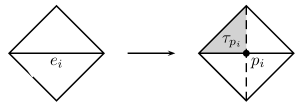
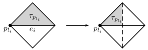
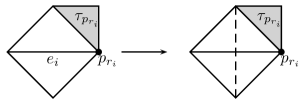
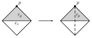
Note that in general Navvsubscriptsuperscript𝑎𝑁𝑣𝑣\mathcal{I}^{a}_{N}v\neq v since the simplex used to define nodal values of Navsubscriptsuperscript𝑎𝑁𝑣\mathcal{I}^{a}_{N}v may not be in the finest mesh 𝒯Nsubscript𝒯𝑁\mathcal{T}_{N} but in 𝒯N1.subscript𝒯𝑁1\mathcal{T}_{N-1}. Figure 4.2 illustrates the choice of σpsubscript𝜎𝑝\sigma_{p} in different cases in 2D.

Refer to caption
(a) Simplex to define (iau)(pi)subscriptsuperscript𝑎𝑖𝑢subscript𝑝𝑖(\mathcal{I}^{a}_{i}u)(p_{i})
Refer to caption
(b) Simplex to define (iau)(pli)subscriptsuperscript𝑎𝑖𝑢subscript𝑝subscript𝑙𝑖(\mathcal{I}^{a}_{i}u)(p_{l_{i}})
Refer to caption
(c) Simplex to define (iau)(pri)subscriptsuperscript𝑎𝑖𝑢subscript𝑝subscript𝑟𝑖(\mathcal{I}^{a}_{i}u)(p_{r_{i}})
Refer to caption
(d) Simplex to define (iau)(p)subscriptsuperscript𝑎𝑖𝑢𝑝(\mathcal{I}^{a}_{i}u)(p)
Figure 4.2. Update of nodal values iausubscriptsuperscript𝑎𝑖𝑢\mathcal{I}^{a}_{i}u to yield i1ausubscriptsuperscript𝑎𝑖1𝑢\mathcal{I}^{a}_{i-1}u: the element τ𝜏\tau chosen to perform the averaging that gives (iau)(p)subscriptsuperscript𝑎𝑖𝑢𝑝(\mathcal{I}^{a}_{i}u)(p) must belong to ωp(𝒯i)subscript𝜔𝑝subscript𝒯𝑖\omega_{p}(\mathcal{T}_{i}). This implies (iai1a)u(p)0subscriptsuperscript𝑎𝑖subscriptsuperscript𝑎𝑖1𝑢𝑝0(\mathcal{I}^{a}_{i}-\mathcal{I}^{a}_{i-1})u(p)\neq 0 possibly for p=pi,pli,pri𝑝subscript𝑝𝑖subscript𝑝subscript𝑙𝑖subscript𝑝subscript𝑟𝑖p=p_{i},p_{l_{i}},p_{r_{i}} and =0absent0=0 otherwise.

4.5. Stable Space Decomposition

Let ϕi,p𝒱(𝒯i)subscriptitalic-ϕ𝑖𝑝𝒱subscript𝒯𝑖\phi_{i,p}\in\mathcal{V}(\mathcal{T}_{i}) denote the nodal basis at node p𝒩(𝒯i).𝑝𝒩subscript𝒯𝑖p\in\mathcal{N}(\mathcal{T}_{i}). Motivated by the stable three-point wavelet construction by Stevenson [42], we define the subspaces 𝒱0=𝒱(𝒯0),subscript𝒱0𝒱subscript𝒯0\mathcal{V}_{0}=\mathcal{V}(\mathcal{T}_{0}), and

𝒱i=span{ϕi,pi,ϕi,pli,ϕi,pri}.subscript𝒱𝑖spansubscriptitalic-ϕ𝑖subscript𝑝𝑖subscriptitalic-ϕ𝑖subscript𝑝subscript𝑙𝑖subscriptitalic-ϕ𝑖subscript𝑝subscript𝑟𝑖\mathcal{V}_{i}={\rm span}\{\phi_{i,p_{i}},\phi_{i,p_{l_{i}}},\phi_{i,p_{r_{i}}}\}.

Let {ϕp:pΛ}conditional-setsubscriptitalic-ϕ𝑝𝑝Λ\{\phi_{p}:p\in\Lambda\} be a basis of 𝒱(𝒯N),𝒱subscript𝒯𝑁\mathcal{V}(\mathcal{T}_{N}), where ΛΛ\Lambda is the index set of the basis functions, and let 𝒱psubscript𝒱𝑝\mathcal{V}_{p} be the 1-dimensional subspace spanned by the nodal bases associated to p𝑝p in the finest grid. We choose the following space decomposition:

𝒱:=pΛ𝒱p+i=0N𝒱i.assign𝒱subscript𝑝Λsubscript𝒱𝑝superscriptsubscript𝑖0𝑁subscript𝒱𝑖\mathcal{V}:=\sum_{p\in\Lambda}\mathcal{V}_{p}+\sum_{i=0}^{N}\mathcal{V}_{i}. (4.3)

Recall that bisubscript𝑏𝑖b_{i} only changes the local patches of two end points of the refinement edge eisubscript𝑒𝑖e_{i} going from 𝒯i1subscript𝒯𝑖1\mathcal{T}_{i-1} to 𝒯i.subscript𝒯𝑖\mathcal{T}_{i}. By construction (iai1a)v(p)=0subscriptsuperscript𝑎𝑖subscriptsuperscript𝑎𝑖1𝑣𝑝0(\mathcal{I}^{a}_{i}-\mathcal{I}^{a}_{i-1})v(p)=0 for p𝒩(𝒯i),ppi,pliformulae-sequence𝑝𝒩subscript𝒯𝑖𝑝subscript𝑝𝑖subscript𝑝subscript𝑙𝑖p\in\mathcal{N}(\mathcal{T}_{i}),p\neq p_{i},p_{l_{i}} or prisubscript𝑝subscript𝑟𝑖p_{r_{i}}, which implies vi:=(iai1a)v𝒱i.assignsubscript𝑣𝑖subscriptsuperscript𝑎𝑖subscriptsuperscript𝑎𝑖1𝑣subscript𝒱𝑖v_{i}:=(\mathcal{I}^{a}_{i}-\mathcal{I}^{a}_{i-1})v\in\mathcal{V}_{i}. Although Navvsubscriptsuperscript𝑎𝑁𝑣𝑣\mathcal{I}^{a}_{N}v\neq v in general, the difference vNav𝑣subscriptsuperscript𝑎𝑁𝑣v-\mathcal{I}^{a}_{N}v is of high frequency in the finest mesh. Let us write vNav=pΛvp𝑣subscriptsuperscript𝑎𝑁𝑣subscript𝑝Λsubscript𝑣𝑝v-\mathcal{I}^{a}_{N}v=\sum_{p\in\Lambda}v_{p} as the basis decomposition. We then obtain a decomposition

v=pΛvp+i=0Nvi,vi𝒱i,formulae-sequence𝑣subscript𝑝Λsubscript𝑣𝑝superscriptsubscript𝑖0𝑁subscript𝑣𝑖subscript𝑣𝑖subscript𝒱𝑖v=\sum_{p\in\Lambda}v_{p}+\sum_{i=0}^{N}v_{i},\quad v_{i}\in\mathcal{V}_{i}, (4.4)

where for convenience we define 1a:=0.assignsubscriptsuperscript𝑎10\mathcal{I}^{a}_{-1}:=0. Moreover, we introduce a subspace 𝒱~:=𝒱H~D1(Ω).assign~𝒱𝒱subscriptsuperscript~𝐻1𝐷Ω\widetilde{\mathcal{V}}:=\mathcal{V}\cap\widetilde{H}^{1}_{D}(\Omega). Then we have the following stable decomposition.

Theorem 4.2 (Stable Decomposition).

Given a triangulation 𝒯N=𝒯0+subscript𝒯𝑁subscript𝒯0\mathcal{T}_{N}=\mathcal{T}_{0}+\mathcal{B} in 𝕋(𝒯0)𝕋subscript𝒯0\mathbb{T}(\mathcal{T}_{0}), let L=maxτ𝒯Ng(τ)𝐿subscript𝜏subscript𝒯𝑁𝑔𝜏L=\max_{\tau\in\mathcal{T}_{N}}g(\tau).

  1. (i)

    For any v𝒱,𝑣𝒱v\in\mathcal{V}, there exist vp𝒱p(pΛ)subscript𝑣𝑝subscript𝒱𝑝𝑝Λv_{p}\in\mathcal{V}_{p}\;(p\in\Lambda) and vi𝒱i(i=1,,N)subscript𝑣𝑖subscript𝒱𝑖𝑖1𝑁v_{i}\in\mathcal{V}_{i}\;(i=1,\cdots,N) such that v=pΛvp+i=0Nvi𝑣subscript𝑝Λsubscript𝑣𝑝superscriptsubscript𝑖0𝑁subscript𝑣𝑖v=\sum_{p\in\Lambda}v_{p}+\sum_{i=0}^{N}v_{i} and

    pΛhp2vp0,a2+v01,a2+i=1Nhi2vi0,a2cd(L)|v|1,a2,less-than-or-similar-tosubscript𝑝Λsuperscriptsubscript𝑝2superscriptsubscriptnormsubscript𝑣𝑝0𝑎2superscriptsubscriptnormsubscript𝑣01𝑎2superscriptsubscript𝑖1𝑁superscriptsubscript𝑖2superscriptsubscriptnormsubscript𝑣𝑖0𝑎2subscript𝑐𝑑𝐿superscriptsubscript𝑣1𝑎2\sum_{p\in\Lambda}h_{p}^{-2}\|v_{p}\|_{0,a}^{2}+\|v_{0}\|_{1,a}^{2}+\sum_{i=1}^{N}h_{i}^{-2}\|v_{i}\|_{0,a}^{2}\lesssim c_{d}(L)|v|_{1,a}^{2}, (4.5)

    where cd(L)={L2,d=22L,d=3.subscript𝑐𝑑𝐿casessuperscript𝐿2𝑑2superscript2𝐿𝑑3c_{d}(L)=\left\{\begin{array}[]{ll}L^{2},&d=2\\ 2^{L},&d=3\end{array}\right..

  2. (ii)

    For any v𝒱~,𝑣~𝒱v\in\widetilde{\mathcal{V}}, there exist vp𝒱p(pΛ)subscript𝑣𝑝subscript𝒱𝑝𝑝Λv_{p}\in\mathcal{V}_{p}\;(p\in\Lambda) and vi𝒱i(i=1,,N)subscript𝑣𝑖subscript𝒱𝑖𝑖1𝑁v_{i}\in\mathcal{V}_{i}\;(i=1,\cdots,N) such that v=pΛvp+i=0Nvi𝑣subscript𝑝Λsubscript𝑣𝑝superscriptsubscript𝑖0𝑁subscript𝑣𝑖v=\sum_{p\in\Lambda}v_{p}+\sum_{i=0}^{N}v_{i} and

    pΛhp2vp0,a2+v01,a2+i=1Nhi2vi0,a2L2|v|1,a2less-than-or-similar-tosubscript𝑝Λsuperscriptsubscript𝑝2superscriptsubscriptnormsubscript𝑣𝑝0𝑎2superscriptsubscriptnormsubscript𝑣01𝑎2superscriptsubscript𝑖1𝑁superscriptsubscript𝑖2superscriptsubscriptnormsubscript𝑣𝑖0𝑎2superscript𝐿2superscriptsubscript𝑣1𝑎2\sum_{p\in\Lambda}h_{p}^{-2}\|v_{p}\|_{0,a}^{2}+\|v_{0}\|_{1,a}^{2}+\sum_{i=1}^{N}h_{i}^{-2}\|v_{i}\|_{0,a}^{2}\lesssim L^{2}|v|_{1,a}^{2} (4.6)
Proof.

The result of (i) is standard. We may use the standard nodal interpolation operator to define a decomposition using the hierarchical basis (cf. [53]).

Now we prove (ii). Given a v𝒱~,𝑣~𝒱v\in\widetilde{\mathcal{V}}, we define v0:=0avassignsubscript𝑣0superscriptsubscript0𝑎𝑣v_{0}:=\mathcal{I}_{0}^{a}v and vi:=(iai1a)v.assignsubscript𝑣𝑖superscriptsubscript𝑖𝑎superscriptsubscript𝑖1𝑎𝑣v_{i}:=(\mathcal{I}_{i}^{a}-\mathcal{I}_{i-1}^{a})v. For vNav=pΛvp,𝑣superscriptsubscript𝑁𝑎𝑣subscript𝑝Λsubscript𝑣𝑝v-\mathcal{I}_{N}^{a}v=\sum_{p\in\Lambda}v_{p}, by the approximability of the quasi-interpolation, cf. (3.6), we have

pΛhp2vp0,a2h1(vNav)0,a2L|v|1,a2.less-than-or-similar-tosubscript𝑝Λsuperscriptsubscript𝑝2subscriptsuperscriptnormsubscript𝑣𝑝20𝑎superscriptsubscriptnormsuperscript1𝑣superscriptsubscript𝑁𝑎𝑣0𝑎2less-than-or-similar-to𝐿superscriptsubscript𝑣1𝑎2\sum_{p\in\Lambda}h_{p}^{-2}\|v_{p}\|^{2}_{0,a}\lesssim\|h^{-1}(v-\mathcal{I}_{N}^{a}v)\|_{0,a}^{2}\lesssim L|v|_{1,a}^{2}. (4.7)

On the other hand, by Theorem 3.5 we obtain

0av1,a2+i=1Nhi2(iai1a)v0,a,ωi2superscriptsubscriptnormsuperscriptsubscript0𝑎𝑣1𝑎2superscriptsubscript𝑖1𝑁superscriptsubscript𝑖2superscriptsubscriptnormsuperscriptsubscript𝑖𝑎superscriptsubscript𝑖1𝑎𝑣0𝑎subscript𝜔𝑖2\displaystyle\left\|\mathcal{I}_{0}^{a}v\right\|_{1,a}^{2}+\sum_{i=1}^{N}h_{i}^{-2}\|(\mathcal{I}_{i}^{a}-\mathcal{I}_{i-1}^{a})v\|_{0,a,\omega_{i}}^{2}
=0av1,a2+l=1Lgi=lhl2(iai1a)v0,a,ωi2absentsuperscriptsubscriptnormsuperscriptsubscript0𝑎𝑣1𝑎2superscriptsubscript𝑙1𝐿subscriptsubscript𝑔𝑖𝑙superscriptsubscript𝑙2superscriptsubscriptnormsuperscriptsubscript𝑖𝑎superscriptsubscript𝑖1𝑎𝑣0𝑎subscript𝜔𝑖2\displaystyle=\left\|\mathcal{I}_{0}^{a}v\right\|_{1,a}^{2}+\sum_{l=1}^{L}\sum_{g_{i}=l}h_{l}^{-2}\|(\mathcal{I}_{i}^{a}-\mathcal{I}_{i-1}^{a})v\|_{0,a,\omega_{i}}^{2}
(i=1L|loghmin|)v1,a2L2|v|1,a2.less-than-or-similar-toabsentsuperscriptsubscript𝑖1𝐿subscriptsuperscriptsubscriptnorm𝑣1𝑎2less-than-or-similar-tosuperscript𝐿2superscriptsubscript𝑣1𝑎2\displaystyle\lesssim\left(\sum_{i=1}^{L}|\log h_{\min}|\right)\|v\|_{1,a}^{2}\lesssim L^{2}|v|_{1,a}^{2}.

Then (4.6) follows by adding the above inequality to inequality (4.7). \Box

Remark 4.3.

The estimate (4.5) is not uniform for d2𝑑2d\geq 2. For d=2𝑑2d=2, L|loghmin|𝐿subscriptL\approx|\log h_{\min}| and the growth of c2(L)subscript𝑐2𝐿c_{2}(L) is acceptable. But for d=3𝑑3d=3, the constant c3(L)=2Lsubscript𝑐3𝐿superscript2𝐿c_{3}(L)=2^{L} grows exponentially. This is the main reason that the hierarchical basis multilevel method deteriorates rapidly in 3D (cf. [58, 7]). For discontinuous coefficients problems, it seems unlikely to find a better decomposition with a better constants; see the counterexamples in [12, 36].

If the coefficients satisfy certain monotonicity, e.g. quasi-monotonicity (cf. [23, 37]) in the local patches, one can show that the interpolation operator defined above is stable in the energy norm without deterioration. \Box

Remark 4.4.

With a close look at the proof of (4.6), we may regroup the vi=(iai1a)vsubscript𝑣𝑖superscriptsubscript𝑖𝑎superscriptsubscript𝑖1𝑎𝑣v_{i}=(\mathcal{I}_{i}^{a}-\mathcal{I}_{i-1}^{a})v into groups l=1LG(l)={1,2,,N}superscriptsubscript𝑙1superscript𝐿𝐺𝑙12𝑁\cup_{l=1}^{L^{\prime}}G(l)=\{1,2,\cdots,N\} such that for any i,jG(l),ωjωi=formulae-sequence𝑖𝑗𝐺𝑙subscript𝜔𝑗subscript𝜔𝑖i,j\in G(l),\omega_{j}\cap\omega_{i}=\varnothing and therefore

i=1Nhi2vi0,a,ωi2superscriptsubscript𝑖1𝑁superscriptsubscript𝑖2superscriptsubscriptnormsubscript𝑣𝑖0𝑎subscript𝜔𝑖2\displaystyle\sum_{i=1}^{N}h_{i}^{-2}\|v_{i}\|_{0,a,\omega_{i}}^{2} =\displaystyle= l=1LjG(l)hj2vj0,a,ωi2L|loghmin||v|1,a2.superscriptsubscript𝑙1superscript𝐿subscript𝑗𝐺𝑙superscriptsubscript𝑗2superscriptsubscriptnormsubscript𝑣𝑗0𝑎subscript𝜔𝑖2superscript𝐿subscriptsuperscriptsubscript𝑣1𝑎2\displaystyle\sum_{l=1}^{L^{\prime}}\sum_{j\in G(l)}h_{j}^{-2}\|v_{j}\|_{0,a,\omega_{i}}^{2}\leq L^{\prime}|\log h_{\min}||v|_{1,a}^{2}.

The constant Lsuperscript𝐿L^{\prime} could be much smaller than L𝐿L; see Section 6 for numerical examples. \Box

4.6. Strengthened Cauchy-Schwarz inequality

An important tool in analysis of the multiplicative preconditioner is the following strengthened Cauchy-Schwarz inequality. A proof can be found in [19, 54].

Lemma 4.5 (Strengthened Cauchy-Schwarz Inequality).

For any ui,vi𝒱i,i=0,1,,N,formulae-sequencesubscript𝑢𝑖subscript𝑣𝑖subscript𝒱𝑖𝑖01𝑁u_{i},v_{i}\in\mathcal{V}_{i},\;\;i=0,1,\cdots,N, we have

|i=0Nj=i+1NA(ui,vj)|(i=0N|ui|1,a2)12(i=0Nhi2vi0,a2)12.less-than-or-similar-tosuperscriptsubscript𝑖0𝑁superscriptsubscript𝑗𝑖1𝑁𝐴subscript𝑢𝑖subscript𝑣𝑗superscriptsuperscriptsubscript𝑖0𝑁superscriptsubscriptsubscript𝑢𝑖1𝑎212superscriptsuperscriptsubscript𝑖0𝑁superscriptsubscript𝑖2superscriptsubscriptnormsubscript𝑣𝑖0𝑎212\left|\sum_{i=0}^{N}\sum_{j=i+1}^{N}A(u_{i},v_{j})\right|\lesssim\left(\sum_{i=0}^{N}|u_{i}|_{1,a}^{2}\right)^{\frac{1}{2}}\left(\sum_{i=0}^{N}h_{i}^{-2}\|v_{i}\|_{0,a}^{2}\right)^{\frac{1}{2}}. (4.8)

As a corollary of (4.8) and the inverse inequality, we have

i=0Nui1,a2i=0Nhi2ui0,a2.less-than-or-similar-tosuperscriptsubscriptnormsuperscriptsubscript𝑖0𝑁subscript𝑢𝑖1𝑎2superscriptsubscript𝑖0𝑁superscriptsubscript𝑖2superscriptsubscriptnormsubscript𝑢𝑖0𝑎2\Big{\|}\sum_{i=0}^{N}u_{i}\Big{\|}_{1,a}^{2}\lesssim\sum_{i=0}^{N}h_{i}^{-2}\|u_{i}\|_{0,a}^{2}. (4.9)

5. Multilevel Preconditioners

In this section, we shall analysis the eigenvalue distribution of the BPX preconditioner and the multigrid V𝑉V-cycle preconditioner on bisection grids, and prove the effective conditioner number is uniformly bounded.

5.1. BPX (Additive) Preconditioner

To simplify the notation, we include 𝒱N+1=𝒱subscript𝒱𝑁1𝒱\mathcal{V}_{N+1}=\mathcal{V} and rewrite our space decomposition as 𝒱=i=0N+1𝒱i.𝒱superscriptsubscript𝑖0𝑁1subscript𝒱𝑖\mathcal{V}=\sum_{i=0}^{N+1}\mathcal{V}_{i}. Based on this space decomposition, we choose SPD smoothers Ri:𝒱i𝒱i:subscript𝑅𝑖subscript𝒱𝑖subscript𝒱𝑖R_{i}:\mathcal{V}_{i}\to\mathcal{V}_{i} satisfying

(Ri1ui,ui)0,ahi2(ui,ui)0,a,ui𝒱i.formulae-sequencesubscriptsuperscriptsubscript𝑅𝑖1subscript𝑢𝑖subscript𝑢𝑖0𝑎subscriptsuperscript2𝑖subscriptsubscript𝑢𝑖subscript𝑢𝑖0𝑎for-allsubscript𝑢𝑖subscript𝒱𝑖(R_{i}^{-1}u_{i},u_{i})_{0,a}\eqsim h^{-2}_{i}(u_{i},u_{i})_{0,a},\;\;\forall u_{i}\in\mathcal{V}_{i}. (5.1)

According to [55], both of the standard Jacobi and symmetric Gauss-Seidel smoother satisfy the above assumption. On the coarsest level, i.e. when i=0𝑖0i=0, we choose the exact solver R0=A01.subscript𝑅0superscriptsubscript𝐴01R_{0}=A_{0}^{-1}. Let Qia:𝒱𝒱i:superscriptsubscript𝑄𝑖𝑎𝒱subscript𝒱𝑖Q_{i}^{a}:\mathcal{V}\to\mathcal{V}_{i} be the weighted L2superscript𝐿2L^{2} projection. Then we can define the BPX-type preconditioner

B=i=0N+1RiQia.𝐵superscriptsubscript𝑖0𝑁1subscript𝑅𝑖superscriptsubscript𝑄𝑖𝑎B=\sum_{i=0}^{N+1}R_{i}Q_{i}^{a}. (5.2)

It is well known [49, 52, 56] that the operator B𝐵B defined by (5.2) is SPD, and

(B1v,v)0,a=infi=0N+1vi=vi=0N+1(Ri1vi,vi)0,a.subscriptsuperscript𝐵1𝑣𝑣0𝑎subscriptinfimumsuperscriptsubscript𝑖0𝑁1subscript𝑣𝑖𝑣superscriptsubscript𝑖0𝑁1subscriptsuperscriptsubscript𝑅𝑖1subscript𝑣𝑖subscript𝑣𝑖0𝑎(B^{-1}v,v)_{0,a}=\inf_{\sum_{i=0}^{N+1}v_{i}=v}\sum_{i=0}^{N+1}(R_{i}^{-1}v_{i},v_{i})_{0,a}. (5.3)

We have the following main result for the BPX preconditioner.

Theorem 5.1.

Given a triangulation 𝒯N=𝒯0+subscript𝒯𝑁subscript𝒯0\mathcal{T}_{N}=\mathcal{T}_{0}+\mathcal{B} in 𝕋(𝒯0)𝕋subscript𝒯0\mathbb{T}(\mathcal{T}_{0}), let L=maxτ𝒯Ng(τ)𝐿subscript𝜏subscript𝒯𝑁𝑔𝜏L=\max_{\tau\in\mathcal{T}_{N}}g(\tau). For the BPX preconditioner defined in (5.2), we have

κ(BA)C1cd(L), and κm0(BA)C0L2.formulae-sequence𝜅𝐵𝐴subscript𝐶1subscript𝑐𝑑𝐿 and subscript𝜅subscript𝑚0𝐵𝐴subscript𝐶0superscript𝐿2\kappa(BA)\leq C_{1}c_{d}(L),\hbox{ and }\kappa_{m_{0}}(BA)\leq C_{0}L^{2}.

Consequently, we have the following convergence estimation of the BPX preconditioned conjugate gradient method:

uukAuu0Asubscriptnorm𝑢subscript𝑢𝑘𝐴subscriptnorm𝑢subscript𝑢0𝐴\displaystyle\frac{\|u-u_{k}\|_{A}}{\|u-u_{0}\|_{A}} \displaystyle\leq 2(C1cd(L)1)m0(C0L1C0L+1)km0.2superscriptsubscript𝐶1subscript𝑐𝑑𝐿1subscript𝑚0superscriptsubscript𝐶0𝐿1subscript𝐶0𝐿1𝑘subscript𝑚0\displaystyle 2\left(C_{1}c_{d}(L)-1\right)^{m_{0}}\left(\frac{C_{0}L-1}{C_{0}L+1}\right)^{k-m_{0}}.
Proof.

First of all, let us estimate λmax(BA).subscript𝜆𝐵𝐴\lambda_{\max}(BA). For any decomposition v=v~+i=0Nvi,v~𝒱,vi𝒱iformulae-sequence𝑣~𝑣superscriptsubscript𝑖0𝑁subscript𝑣𝑖formulae-sequence~𝑣𝒱subscript𝑣𝑖subscript𝒱𝑖v=\tilde{v}+\sum_{i=0}^{N}v_{i},\tilde{v}\in\mathcal{V},v_{i}\in\mathcal{V}_{i}, we have

vA2superscriptsubscriptnorm𝑣𝐴2\displaystyle\|v\|_{A}^{2} v~A2+i=0NviA2h1v~0,a2+i=0Nhi2vi0,a2i=0N+1(Ri1vi,vi)0,a.less-than-or-similar-toabsentsuperscriptsubscriptnorm~𝑣𝐴2superscriptsubscriptnormsuperscriptsubscript𝑖0𝑁subscript𝑣𝑖𝐴2superscriptsubscriptnormsuperscript1~𝑣0𝑎2superscriptsubscript𝑖0𝑁superscriptsubscript𝑖2superscriptsubscriptnormsubscript𝑣𝑖0𝑎2superscriptsubscript𝑖0𝑁1subscriptsuperscriptsubscript𝑅𝑖1subscript𝑣𝑖subscript𝑣𝑖0𝑎\displaystyle\lesssim\|\tilde{v}\|_{A}^{2}+\Big{\|}\sum_{i=0}^{N}v_{i}\Big{\|}_{A}^{2}\leq\|h^{-1}\tilde{v}\|_{0,a}^{2}+\sum_{i=0}^{N}h_{i}^{-2}\|v_{i}\|_{0,a}^{2}\leq\sum_{i=0}^{N+1}(R_{i}^{-1}v_{i},v_{i})_{0,a}.

In the second step, we used the inverse inequality and the inequality (4.9). In the third step, we used the assumption (5.1) of Risubscript𝑅𝑖R_{i} . Taking infimum, we get

vA2infi=0N+1vi=vi=0N+1(Ri1vi,vi)0,a=(B1v,v)0,a,less-than-or-similar-tosuperscriptsubscriptnorm𝑣𝐴2subscriptinfimumsuperscriptsubscript𝑖0𝑁1subscript𝑣𝑖𝑣superscriptsubscript𝑖0𝑁1subscriptsuperscriptsubscript𝑅𝑖1subscript𝑣𝑖subscript𝑣𝑖0𝑎subscriptsuperscript𝐵1𝑣𝑣0𝑎\|v\|_{A}^{2}\lesssim\inf_{\sum_{i=0}^{N+1}v_{i}=v}\sum_{i=0}^{N+1}(R_{i}^{-1}v_{i},v_{i})_{0,a}=(B^{-1}v,v)_{0,a},

which implies that λmax(BA)1.less-than-or-similar-tosubscript𝜆𝐵𝐴1\lambda_{\max}(BA)\lesssim 1.

To estimate λmin,subscript𝜆\lambda_{\min}, in view of (5.3) we choose the decomposition as in the stable decomposition Theorem 4.2 (see (4.5)) to conclude that

(B1v,v)0,ai=0N+1(Ri1vi,vi)0,acd(L)(Av,v)0,a,subscriptsuperscript𝐵1𝑣𝑣0𝑎superscriptsubscript𝑖0𝑁1subscriptsuperscriptsubscript𝑅𝑖1subscript𝑣𝑖subscript𝑣𝑖0𝑎less-than-or-similar-tosubscript𝑐𝑑𝐿subscript𝐴𝑣𝑣0𝑎(B^{-1}v,v)_{0,a}\leq\sum_{i=0}^{N+1}(R_{i}^{-1}v_{i},v_{i})_{0,a}\lesssim c_{d}(L)(Av,v)_{0,a},

which implies that λmin(BA)cd(L).greater-than-or-equivalent-tosubscript𝜆𝐵𝐴subscript𝑐𝑑𝐿\lambda_{\min}(BA)\gtrsim c_{d}(L). Therefore we have κ(BA)cd(L).less-than-or-similar-to𝜅𝐵𝐴subscript𝑐𝑑𝐿\kappa(BA)\lesssim c_{d}(L).

On the other hand, if we apply (4.6) in the subspace 𝒱~𝒱,~𝒱𝒱\widetilde{\mathcal{V}}\subset\mathcal{V}, we obtain λm0+1(BA)L2greater-than-or-equivalent-tosubscript𝜆subscript𝑚01𝐵𝐴superscript𝐿2\lambda_{m_{0}+1}(BA)\gtrsim L^{2} by the “min-max” Theorem 2.3. Hence we get an estimate of the effective condition number κm0(BA)L2.less-than-or-similar-tosubscript𝜅subscript𝑚0𝐵𝐴superscript𝐿2\kappa_{m_{0}}(BA)\lesssim L^{2}. The convergence rate estimate then follows by Theorem 2.1. This completes the proof. \Box

From this convergence result, we can see that the convergence rate will deteriorate a little bit by cd(L)subscript𝑐𝑑𝐿c_{d}(L) as L𝐿L grows. But since m0subscript𝑚0m_{0} is a fixed number, when k𝑘k grows, the convergence rate will be controlled by the effective condition number, which is bounded uniformly with respect to the coefficient and logarithmically with respect to the mesh size. Notice that L|loghmin|𝐿subscriptL\eqsim|\log h_{\min}| and thus the asymptotic convergence rate of the PCG algorithm is 11C|loghmin|11𝐶subscript1-\frac{1}{C|\log h_{\min}|} for h<1.1h<1.

Remark 5.2.

The estimate κ(BA)C1cd(L)𝜅𝐵𝐴subscript𝐶1subscript𝑐𝑑𝐿\kappa(BA)\leq C_{1}c_{d}(L) is sharp in the sense that there exists an example on BPX preconditioner such that κ(BA)cd(L)𝜅𝐵𝐴subscript𝑐𝑑𝐿\kappa(BA)\eqsim c_{d}(L) (cf. [36]). \Box

Remark 5.3.

Here we should emphasize that the convergence rate estimate in Theorem 5.1 holds for general substructures. In some special circumstance, for example “edge type” or “exceptional” in the terminology in  [36], or “quasi-monotone” coefficient in  [23], we can sharpen the convergence estimate in Theorem 5.1 by a modification of Theorem 4.2, see [36]. \Box

5.2. Multigrid (Multiplicative) Preconditioner

We shall use the following symmetric V-cycle multigrid as a preconditioner in the PCG method and prove the efficiency of such a method. Let Ai:=A|𝒱i.assignsubscript𝐴𝑖evaluated-at𝐴subscript𝒱𝑖A_{i}:=A|_{\mathcal{V}_{i}}. Then one step of the standard V𝑉V-cycle multigrid B:𝒱𝒱:𝐵𝒱𝒱B:\mathcal{V}\to\mathcal{V} is recursively defined as follows:

Let B0=A01,subscript𝐵0superscriptsubscript𝐴01B_{0}=A_{0}^{-1}, for i>0𝑖0i>0 and g𝒱i,𝑔subscript𝒱𝑖g\in\mathcal{V}_{i}, define Big=w3.subscript𝐵𝑖𝑔subscript𝑤3B_{i}g=w_{3}. (i) Presmoothing : w1=Rig;subscript𝑤1subscript𝑅𝑖𝑔w_{1}=R_{i}g; (ii) Correction: w2=w1+Bi1Qi1(gAiw1);subscript𝑤2subscript𝑤1subscript𝐵𝑖1subscript𝑄𝑖1𝑔subscript𝐴𝑖subscript𝑤1w_{2}=w_{1}+B_{i-1}Q_{i-1}(g-A_{i}w_{1}); (iii) Postsmoothing: w3=w2+Ri(gAiw2).subscript𝑤3subscript𝑤2superscriptsubscript𝑅𝑖𝑔subscript𝐴𝑖subscript𝑤2w_{3}=w_{2}+R_{i}^{*}(g-A_{i}w_{2}). Set B=BN+1.𝐵subscript𝐵𝑁1B=B_{N+1}.

For simplicity, we focus on the case of exact subspace solver, i.e., Ri=Ai1subscript𝑅𝑖superscriptsubscript𝐴𝑖1R_{i}=A_{i}^{-1} for i=0,,N𝑖0𝑁i=0,\cdots,N and for the finest level, RN+1subscript𝑅𝑁1R_{N+1} is chosen as Gauss-Seidel smoother, which can be also understood as the multiplicative method with exact local solvers applied to the nodal decomposition [51]. Let Pp:𝒱𝒱p:subscript𝑃𝑝𝒱subscript𝒱𝑝P_{p}:\mathcal{V}\to\mathcal{V}_{p} and Pi:𝒱𝒱i:subscript𝑃𝑖𝒱subscript𝒱𝑖P_{i}:\mathcal{V}\to\mathcal{V}_{i} be the orthogonal projection with respect to the inner product (,)asubscript𝑎(\cdot,\cdot)_{a}. For our special choices of smoothers, we then have

IRN+1A𝐼subscript𝑅𝑁1𝐴\displaystyle I-R_{N+1}A =pΛ(IPp),absentsubscriptproduct𝑝Λ𝐼subscript𝑃𝑝\displaystyle=\prod_{p\in\Lambda}(I-P_{p}),
IBNA𝐼subscript𝐵𝑁𝐴\displaystyle I-B_{N}A =(i=0N(IPi))(i=0N(IPi)),absentsuperscriptsuperscriptsubscriptproduct𝑖0𝑁𝐼subscript𝑃𝑖superscriptsubscriptproduct𝑖0𝑁𝐼subscript𝑃𝑖\displaystyle=\left(\prod_{i=0}^{N}(I-P_{i})\right)^{*}\left(\prod_{i=0}^{N}(I-P_{i})\right),
IBAAsubscriptnorm𝐼𝐵𝐴𝐴\displaystyle\left\|I-BA\right\|_{A} =i=0N(IPi)pΛ(IPp)A2.absentsuperscriptsubscriptnormsuperscriptsubscriptproduct𝑖0𝑁𝐼subscript𝑃𝑖subscriptproduct𝑝Λ𝐼subscript𝑃𝑝𝐴2\displaystyle=\left\|\prod_{i=0}^{N}(I-P_{i})\prod_{p\in\Lambda}(I-P_{p})\right\|_{A}^{2}.

For exact local solvers, we can apply the crucial X-Z identity [56] to conclude

IBAA=111+c0,subscriptnorm𝐼𝐵𝐴𝐴111subscript𝑐0\left\|I-BA\right\|_{A}=1-\frac{1}{1+c_{0}}, (5.4)

where

c0=supvA=1infv=pΛvp+i=0Nvi(i=0NPij=i+1Nvj+PipΛvpA2+pΛPpq>pvqA2).subscript𝑐0subscriptsupremumsubscriptnorm𝑣𝐴1subscriptinfimum𝑣subscript𝑝Λsubscript𝑣𝑝superscriptsubscript𝑖0𝑁subscript𝑣𝑖superscriptsubscript𝑖0𝑁subscriptsuperscriptnormsubscript𝑃𝑖superscriptsubscript𝑗𝑖1𝑁subscript𝑣𝑗subscript𝑃𝑖subscript𝑝Λsubscript𝑣𝑝2𝐴subscript𝑝Λsuperscriptsubscriptnormsubscript𝑃𝑝subscript𝑞𝑝subscript𝑣𝑞𝐴2\displaystyle c_{0}=\sup_{\left\|v\right\|_{A}=1}\inf_{v=\sum_{p\in\Lambda}v_{p}+\sum_{i=0}^{N}v_{i}}\left(\sum_{i=0}^{N}\Big{\|}P_{i}\sum_{j=i+1}^{N}v_{j}+P_{i}\sum_{p\in\Lambda}v_{p}\Big{\|}^{2}_{A}+\sum_{p\in\Lambda}\big{\|}P_{p}\sum_{q>p}v_{q}\big{\|}_{A}^{2}\right).
Theorem 5.4.

Given a triangulation 𝒯N=𝒯0+subscript𝒯𝑁subscript𝒯0\mathcal{T}_{N}=\mathcal{T}_{0}+\mathcal{B} in 𝕋(𝒯0)𝕋subscript𝒯0\mathbb{T}(\mathcal{T}_{0}), let L=maxτ𝒯Ng(τ)𝐿subscript𝜏subscript𝒯𝑁𝑔𝜏L=\max_{\tau\in\mathcal{T}_{N}}g(\tau). For the multigrid V𝑉V-cycle preconditioner B𝐵B, we have

κ(BA)cd(L),κm0(BA)L2.formulae-sequenceless-than-or-similar-to𝜅𝐵𝐴subscript𝑐𝑑𝐿less-than-or-similar-tosubscript𝜅subscript𝑚0𝐵𝐴superscript𝐿2\kappa(BA)\lesssim c_{d}(L),\;\;\kappa_{m_{0}}(BA)\lesssim L^{2}.

Consequently, we have the following the convergence rate estimate of the BPX preconditioned conjugate gradient method:

uukAuu0Asubscriptnorm𝑢subscript𝑢𝑘𝐴subscriptnorm𝑢subscript𝑢0𝐴\displaystyle\frac{\|u-u_{k}\|_{A}}{\|u-u_{0}\|_{A}} \displaystyle\leq 2(C1cd(L)1)m0(C0L1C0L+1)km0.2superscriptsubscript𝐶1subscript𝑐𝑑𝐿1subscript𝑚0superscriptsubscript𝐶0𝐿1subscript𝐶0𝐿1𝑘subscript𝑚0\displaystyle 2\left(C_{1}c_{d}(L)-1\right)^{m_{0}}\left(\frac{C_{0}L-1}{C_{0}L+1}\right)^{k-m_{0}}.
Proof.

Since IBA𝐼𝐵𝐴I-BA is a non-expansive operator, we conclude λmax(BA)1subscript𝜆𝐵𝐴1\lambda_{\max}(BA)\leq 1. Since IBA𝐼𝐵𝐴I-BA is SPD in the A𝐴A-inner product and λmax(BA)1subscript𝜆𝐵𝐴1\lambda_{\max}(BA)\leq 1, we have

IBAAsubscriptnorm𝐼𝐵𝐴𝐴\displaystyle\|I-BA\|_{A} =\displaystyle= max{|1λmin(BA)|,|1λmax(BA)|}=1λmin(BA).1subscript𝜆𝐵𝐴1subscript𝜆𝐵𝐴1subscript𝜆𝐵𝐴\displaystyle\max\{|1-\lambda_{\min}(BA)|,|1-\lambda_{\max}(BA)|\}=1-\lambda_{\min}(BA).

To get an estimate on the minimum eigenvalue of BA𝐵𝐴BA, we only need to get a upper bound of the constant c0subscript𝑐0c_{0} in (5.4).

To do so, for any v𝒱𝑣𝒱v\in\mathcal{V}, we chose the decomposition in Theorem 4.2. That is,

v=v~+i=1Nvi, with v0=0av,vi=(iai1a)v,formulae-sequence𝑣~𝑣superscriptsubscript𝑖1𝑁subscript𝑣𝑖formulae-sequence with subscript𝑣0superscriptsubscript0𝑎𝑣subscript𝑣𝑖superscriptsubscript𝑖𝑎superscriptsubscript𝑖1𝑎𝑣v=\tilde{v}+\sum_{i=1}^{N}v_{i},\mbox{ with }v_{0}=\mathcal{I}_{0}^{a}v,\;\;v_{i}=(\mathcal{I}_{i}^{a}-\mathcal{I}_{i-1}^{a})v,

where v~=vNav=pΛvp.~𝑣𝑣superscriptsubscript𝑁𝑎𝑣subscript𝑝Λsubscript𝑣𝑝\tilde{v}=v-\mathcal{I}_{N}^{a}v=\sum_{p\in\Lambda}v_{p}. Then by shape regularity of the triangulation, we have

c0i=0NPij=i+1NvjA2+i=0NPiv~A2+pΛPpq>pvqA2.less-than-or-similar-tosubscript𝑐0superscriptsubscript𝑖0𝑁superscriptsubscriptnormsubscript𝑃𝑖superscriptsubscript𝑗𝑖1𝑁subscript𝑣𝑗𝐴2superscriptsubscript𝑖0𝑁superscriptsubscriptnormsubscript𝑃𝑖~𝑣𝐴2subscript𝑝Λsuperscriptsubscriptnormsubscript𝑃𝑝subscript𝑞𝑝subscript𝑣𝑞𝐴2c_{0}\lesssim\sum_{i=0}^{N}\Big{\|}P_{i}\sum_{j=i+1}^{N}v_{j}\Big{\|}_{A}^{2}+\sum_{i=0}^{N}\left\|P_{i}\tilde{v}\right\|_{A}^{2}+\sum_{p\in\Lambda}\left\|P_{p}\sum_{q>p}v_{q}\right\|_{A}^{2}.

We estimate these three terms as follows. For the last term, by the finite overlapping of nodal bases, we have

pΛPpq>pvqA2subscript𝑝Λsuperscriptsubscriptnormsubscript𝑃𝑝subscript𝑞𝑝subscript𝑣𝑞𝐴2\displaystyle\sum_{p\in\Lambda}\big{\|}P_{p}\sum_{q>p}v_{q}\big{\|}_{A}^{2} less-than-or-similar-to\displaystyle\lesssim pΛq>pvqA,ωp2subscript𝑝Λsuperscriptsubscriptnormsubscript𝑞𝑝subscript𝑣𝑞𝐴subscript𝜔𝑝2\displaystyle\sum_{p\in\Lambda}\big{\|}\sum_{q>p}v_{q}\big{\|}_{A,\omega_{p}}^{2}
less-than-or-similar-to\displaystyle\lesssim pΛvpA,ωp2pΛhp2vp0,a,ωp2less-than-or-similar-tosubscript𝑝Λsuperscriptsubscriptnormsubscript𝑣𝑝𝐴subscript𝜔𝑝2subscript𝑝Λsuperscriptsubscript𝑝2superscriptsubscriptnormsubscript𝑣𝑝0𝑎subscript𝜔𝑝2\displaystyle\sum_{p\in\Lambda}\|v_{p}\|_{A,\omega_{p}}^{2}\lesssim\sum_{p\in\Lambda}h_{p}^{-2}\|v_{p}\|_{0,a,\omega_{p}}^{2}
less-than-or-similar-to\displaystyle\lesssim h1(vNav)0,a2vA2.less-than-or-similar-tosuperscriptsubscriptnormsuperscript1𝑣superscriptsubscript𝑁𝑎𝑣0𝑎2superscriptsubscriptnorm𝑣𝐴2\displaystyle\|h^{-1}(v-\mathcal{I}_{N}^{a}v)\|_{0,a}^{2}\lesssim\|v\|_{A}^{2}.

For the middle term, we regroup by generations and use (4.2) to get

i=0NPiv~A2superscriptsubscript𝑖0𝑁superscriptsubscriptnormsubscript𝑃𝑖~𝑣𝐴2\displaystyle\sum_{i=0}^{N}\Big{\|}P_{i}\tilde{v}\Big{\|}_{A}^{2} =\displaystyle= k=0Ll,gl=kPlv~A2k=0Ll,gl=kv~A,ω~l2superscriptsubscript𝑘0𝐿subscript𝑙subscript𝑔𝑙𝑘superscriptsubscriptnormsubscript𝑃𝑙~𝑣𝐴2superscriptsubscript𝑘0𝐿subscript𝑙subscript𝑔𝑙𝑘superscriptsubscriptnorm~𝑣𝐴subscript~𝜔𝑙2\displaystyle\sum_{k=0}^{L}\sum_{l,g_{l}=k}\Big{\|}P_{l}\tilde{v}\Big{\|}_{A}^{2}\leq\sum_{k=0}^{L}\sum_{l,g_{l}=k}\|\tilde{v}\|_{A,\tilde{\omega}_{l}}^{2}
less-than-or-similar-to\displaystyle\lesssim k=0Lv~A2=Lv~A2.superscriptsubscript𝑘0𝐿superscriptsubscriptnorm~𝑣𝐴2𝐿superscriptsubscriptnorm~𝑣𝐴2\displaystyle\sum_{k=0}^{L}\|\tilde{v}\|_{A}^{2}=L\|\tilde{v}\|_{A}^{2}.

For the first term, we define ui=Pi(j=i+1Nvj)subscript𝑢𝑖subscript𝑃𝑖superscriptsubscript𝑗𝑖1𝑁subscript𝑣𝑗u_{i}=P_{i}\left(\sum_{j=i+1}^{N}v_{j}\right) and u0:=P0(vv0)assignsubscript𝑢0subscript𝑃0𝑣subscript𝑣0u_{0}:=P_{0}(v-v_{0}) and apply the strengthened Cauchy Schwarz inequality, cf. Lemma 4.5 to get

i=0NPij=i+1NvjA2superscriptsubscript𝑖0𝑁superscriptsubscriptnormsubscript𝑃𝑖superscriptsubscript𝑗𝑖1𝑁subscript𝑣𝑗𝐴2\displaystyle\sum_{i=0}^{N}\Big{\|}P_{i}\sum_{j=i+1}^{N}v_{j}\Big{\|}_{A}^{2} =\displaystyle= i=0Nj=i+1NA(ui,vj)superscriptsubscript𝑖0𝑁superscriptsubscript𝑗𝑖1𝑁𝐴subscript𝑢𝑖subscript𝑣𝑗\displaystyle\sum_{i=0}^{N}\sum_{j=i+1}^{N}A(u_{i},v_{j})
less-than-or-similar-to\displaystyle\lesssim vv0A2+i=1Nhi2vi0,a2superscriptsubscriptnorm𝑣subscript𝑣0𝐴2superscriptsubscript𝑖1𝑁superscriptsubscript𝑖2superscriptsubscriptnormsubscript𝑣𝑖0𝑎2\displaystyle\|v-v_{0}\|_{A}^{2}+\sum_{i=1}^{N}h_{i}^{-2}\|v_{i}\|_{0,a}^{2}
less-than-or-similar-to\displaystyle\lesssim cd(L)vA2.subscript𝑐𝑑𝐿superscriptsubscriptnorm𝑣𝐴2\displaystyle c_{d}(L)\|v\|_{A}^{2}.

Here the constant cd(L)subscript𝑐𝑑𝐿c_{d}(L) can be improved to L2superscript𝐿2L^{2} if we consider the decomposition (4.6) of v𝒱~.𝑣~𝒱v\in\widetilde{\mathcal{V}}. Combined with the Mini-Max Theorem 2.3, yields

λmin(BA)cd(L),λm0+1(BA)L2,formulae-sequencegreater-than-or-equivalent-tosubscript𝜆𝐵𝐴subscript𝑐𝑑𝐿greater-than-or-equivalent-tosubscript𝜆subscript𝑚01𝐵𝐴superscript𝐿2\lambda_{\min}(BA)\gtrsim c_{d}(L),\;\;\lambda_{m_{0}+1}(BA)\gtrsim L^{-2},

and thus

κ(BA)cd(L),κm0(BA)L2.formulae-sequenceless-than-or-similar-to𝜅𝐵𝐴subscript𝑐𝑑𝐿less-than-or-similar-tosubscript𝜅subscript𝑚0𝐵𝐴superscript𝐿2\kappa(BA)\lesssim c_{d}(L),\quad\kappa_{m_{0}}(BA)\lesssim L^{2}.

Finally, the convergence rate of the PCG method follows by Theorem 2.1. \Box

Follow the same proof as Theorem 5.4, we can also obtain the following convergence result for the local multigrid V𝑉V-cycle solver.

Corollary 5.5.

For the multigrid V𝑉V-cycle algorithm defined above on bisection grids, we have

EA=IBAA=111+c0,subscriptnorm𝐸𝐴subscriptnorm𝐼𝐵𝐴𝐴111subscript𝑐0\|E\|_{A}=\|I-BA\|_{A}=1-\frac{1}{1+c_{0}},

where c0cd(L).less-than-or-similar-tosubscript𝑐0subscript𝑐𝑑𝐿c_{0}\lesssim c_{d}(L).

This corollary implies that multigrid alone is not robust, especially in 3D. In this case, the convergence rate of multigrid will be proportional to 12L1hmin1,similar-to-or-equals1superscript2𝐿1subscriptsuperscript11-2^{-L}\simeq 1-h^{-1}_{\min}, which deteriorates rapidly as the mesh size become small. Remark 5.3 is also applicable here, i.e., all the above estimates are estimates for the worst case. For the special circumstances mentioned in Remark 5.3, the estimates can be improved in the same way.

6. Numerical Experiments

In this section, we present some numerical experiments to support the theoretical results in previous sections. In the implementation of the adaptive loop, we use a modification of the error indicator presented in [37]. Some other a posteriori error indicators for jump coefficients problem (1.1) can be found in [9, 21, 44, 14]. The adaptive algorithm using different error indicators will generate different grids. However, we emphasize that the robustness of the local adaptive multilevel preconditioners is independent of how the grids are generated in the refinement procedure.

The implementation of the BPX preconditioner and the multigrid methods are standard, and can be found in, for example, [13, 53]. The implementation of the PCG algorithm can be found in [24, 38]. All numerical examples are implemented by using i𝑖iFEM [18]. We only present three-dimensional examples here and refer to [20] for two-dimensional ones. In the PCG algorithm, we use the stopping criterion

ukuk1AukA1010.subscriptnormsuperscript𝑢𝑘superscript𝑢𝑘1𝐴subscriptnormsuperscript𝑢𝑘𝐴superscript1010\frac{\|u^{k}-u^{k-1}\|_{A}}{\|u^{k}\|_{A}}\leq 10^{-10}.

In the implementation of the local multilevel preconditioners, we use an algorithm for coarsening bisection grids introduced by [20] for two dimensional case and [18] for three dimensional one. The coarsening algorithm will find all compatible bisections and regroup them, with possibly different generations, into groups l=1LG(l)={1,2,,N}superscriptsubscript𝑙1superscript𝐿𝐺𝑙12𝑁\cup_{l=1}^{L^{\prime}}G(l)=\{1,2,\cdots,N\} such that for any i,jG(l),ωjωi=.formulae-sequence𝑖𝑗𝐺𝑙subscript𝜔𝑗subscript𝜔𝑖i,j\in G(l),\omega_{j}\cap\omega_{i}=\varnothing. Each coarsening step is corresponding to a level in the multilevel terminology, and the total number of levels is L.superscript𝐿L^{\prime}. There are two major benefits of using this coarsening algorithm.

  1. (i)

    We do not need to store the complex bisection tree structure of the refinement procedure explicitly in the algorithm. Instead, we only need the grid information on the finest level and the coarsening subroutine will restore multilevel structure.

  2. (ii)

    Our numerical evidence shows that the number of nodes will decrease around one half in one coarsening step. Therefore the constant Lsuperscript𝐿L^{\prime} is much smaller than the maximal generation L|loghmin|𝐿subscriptL\eqsim|\log h_{\min}|.

In what follows, we will use some shorthand notation for the different algorithms implemented.

  • TPSMG stands for the V𝑉V-cycle multigrid with Three-Point Smoothing (TPS), which only performs smoothing on new vertices and their two direct neighbors sharing the same edge.

  • TPSMGCG is the PCG algorithm using the TPSMG as preconditioner.

  • TPSBPXCG is the additive version of TPSMG preconditioner.

Among all these algorithms, the main focus of this paper is the behavior of TPSMGCG and TPSBPXCG. In the numerical experiments below, we also report some results for TPSMG for comparison.

Inspired by [36, 50, 55], we consider solving the model equation (1.1) in the cubic domain Ω=(1,1)3.Ωsuperscript113\Omega=(-1,1)^{3}. Let the coefficient a(x)𝑎𝑥a(x) be the constants a1=a2=1subscript𝑎1subscript𝑎21a_{1}=a_{2}=1 and a3=εsubscript𝑎3𝜀a_{3}=\varepsilon on the three regions Ω1,Ω2subscriptΩ1subscriptΩ2\Omega_{1},\;\Omega_{2} and Ω3subscriptΩ3\Omega_{3} respectively (see Figure 6.1), where

Ω1=(0.5,0)3,Ω2=(0,0.5)3 and Ω3=Ω(Ω¯1Ω¯2).formulae-sequencesubscriptΩ1superscript0.503subscriptΩ2superscript00.53 and subscriptΩ3Ωsubscript¯Ω1subscript¯Ω2\Omega_{1}=(-0.5,0)^{3},\Omega_{2}=(0,0.5)^{3}\;\hbox{ and }\;\Omega_{3}=\Omega\setminus(\overline{\Omega}_{1}\cup\overline{\Omega}_{2}).
Refer to caption
Figure 6.1. The coefficients a1=a2=1subscript𝑎1subscript𝑎21a_{1}=a_{2}=1 in the gray domains Ω1subscriptΩ1\Omega_{1} and Ω2,subscriptΩ2\Omega_{2}, and a3=εsubscript𝑎3𝜀a_{3}=\varepsilon in the rest of the domain.

We choose f=1𝑓1f=1 and impose the following boundary conditions: Dirichlet conditions

u{1}×[1,1]×[1,1]=0,u{1}×[1,1]×[1,1]=1,formulae-sequencesubscript𝑢111110subscript𝑢111111u_{\{-1\}\times[-1,1]\times[-1,1]}=0,\quad u_{\{1\}\times[-1,1]\times[-1,1]}=1,

and homogenous Neumann boundary conditions on the remaining boundary. For this problem, singularities occur along edges of Ω1subscriptΩ1\Omega_{1} and Ω2subscriptΩ2\Omega_{2}. Figure 6.2 shows an adaptive mesh and the corresponding finite element approximation after several iterations of the adaptive algorithm. To view the mesh around the singularity, we only show half of the domain Ω.Ω\Omega.
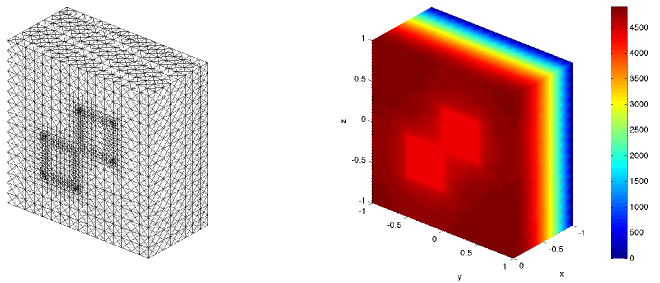
Refer to caption
Figure 6.2. An adaptive mesh and finite element solution with ε=104𝜀superscript104\varepsilon=10^{-4} and 364663646636466 vertices.

Tables 6.16.4 give comparisons of the number of iterations for three different algorithms: TPSMG, TPSMGCG and TPSBPXCG algorithms, respectively, with the choice of ε=104,102,102𝜀superscript104superscript102superscript102\varepsilon=10^{-4},10^{-2},10^{2} and 104superscript10410^{4}. As we observe from these tables, the number of iterations for TPSMG algorithm grows rapidly as the mesh is refined when ε𝜀\varepsilon is small. On the other hand, the number of iterations for TPSMGCG and TPSBPXCG is very robust and only grows a little bit when the mesh is refined, as we expected from the theory. We also observe that if ε𝜀\varepsilon is large, the TPSMG algorithm will converge uniformly. This is because the coefficient in Ω3subscriptΩ3\Omega_{3}, which contains the Dirichlet boundary, is dominant. In this case, we could use the standard multigrid analysis (as in [51]) to show the robustness of the preconditioners.

DOF TPSMG TPSMGCG TPSBPXCG
4913 41 13 18
5505 62 15 18
6617 89 18 21
8666 99 19 19
10585 98 19 20
12411 125 23 25
16353 154 23 23
21248 182 22 23
27755 197 26 32
36466 178 27 29
43271 238 25 30
51163 283 28 36
72349 395 32 34
89146 424 31 34
104747 413 34 38
Table 6.1. Comparison of Number of Iterations for TPSMG, TPSMGCG and TPSBPXCG when ε=104𝜀superscript104\varepsilon=10^{-4}.
DOF TPSMG TPSMGCG TPSBPXCG
4913 46 13 17
5550 51 15 17
6743 61 17 20
8907 65 16 19
10729 66 17 20
13281 86 20 24
17146 90 20 21
23139 90 20 24
28613 160 25 29
37338 175 24 27
43610 149 22 26
52715 154 25 31
72967 238 28 29
89320 165 25 33
113131 294 30 38
Table 6.2. Comparison of Number of Iterations for TPSMG, TPSMGCG and TPSBPXCG when ε=102𝜀superscript102\varepsilon=10^{-2}.
DOF TPSMG TPSMGCG TPSBPXCG
4913 16 10 14
5279 37 15 15
5867 43 17 18
6522 48 16 19
7562 68 17 18
9493 61 17 18
11858 49 15 18
15257 68 15 18
20649 61 16 19
27946 49 17 21
36735 52 16 20
48890 58 16 22
68297 71 18 22
89872 55 16 21
119109 61 17 23
Table 6.3. Comparison of Number of Iterations for TPSMG, TPSMGCG and TPSBPXCG when ε=102𝜀superscript102\varepsilon=10^{2}.
DOF TPSMG TPSMGCG TPSBPXCG
4913 16 10 14
5269 37 15 15
5863 42 17 18
6493 45 16 18
7531 68 17 18
9419 59 16 17
11721 46 15 18
14941 69 15 18
20065 59 16 19
27199 47 17 21
35601 59 16 20
47743 55 16 22
66989 71 18 21
88079 57 16 21
116739 56 17 23
Table 6.4. Comparison of Number of Iterations for TPSMG, TPSMGCG and TPSBPXCG when ε=104𝜀superscript104\varepsilon=10^{4}.

Figure 6.3 shows the eigenvalue distributions for the TPSMGCG and TPSBPXCG preconditioned systems. As we can see from the figure, there is one small eigenvalue for both preconditioned systems. This agrees with the theoretical results, the number of small eigenvalues is bounded by the number of floating subdomains m02.subscript𝑚02m_{0}\equiv 2.
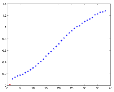
Refer to caption
(a) Eigenvalues for TPSBPXCG
Refer to caption
(b) Eigenvalues for TPSMGCG
Figure 6.3. Example 2: Eigenvalues of BA𝐵𝐴BA when ε=104𝜀superscript104\varepsilon=10^{-4} with 124111241112411 vertices

Figure 6.4 shows the condition number and effective condition number of TPSBPXCG and TPSMGCG preconditioned systems. From Figure 6.4, we observed that when ε𝜀\varepsilon is small, the condition number deteriorates (κ(BA)[3,1100]𝜅𝐵𝐴31100\kappa(BA)\in[3,1100] for TPSBPXCG, and κ(BA)[3,125]𝜅𝐵𝐴3125\kappa(BA)\in[3,125] for TPSMGCG as we can see from the figure). On the other hand, if we get rid of the first small eigenvalue, the effective condition number κ1(BA)subscript𝜅1𝐵𝐴\kappa_{1}(BA) of TPSBPXCG and TPSMGCG preconditioned systems (the black and red lines, respectively) are almost identical for different ε.𝜀\varepsilon. This indicates that the effective condition numbers are uniform with respect to the jumps. Moreover, as we can see from Figure 6.4, κ1(BA)subscript𝜅1𝐵𝐴\kappa_{1}(BA) are mildly increasing with respect to the DOFs (κ1(BA)[1,80]subscript𝜅1𝐵𝐴180\kappa_{1}(BA)\in[1,80] for TPSBPXCG, and κ1(BA)[1,30]subscript𝜅1𝐵𝐴130\kappa_{1}(BA)\in[1,30] for TPSMGCG).These results agree with our theoretical expectations from Section 5.
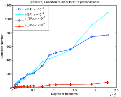
Refer to caption
(a) TPSBPXCG
Refer to caption
(b) TPSMGCG
Figure 6.4. Example 2: κ(BA)𝜅𝐵𝐴\kappa(BA) and κ1(BA)subscript𝜅1𝐵𝐴\kappa_{1}(BA) for the cases ε=106,104𝜀superscript106superscript104\varepsilon=10^{-6},10^{-4} w.r.t the DOFs.

7. Conclusion

In this paper, we designed local multilevel preconditioners based on the decomposition of the finite element space into 3-point subspaces for the highly graded mesh obtained from adaptive bisection algorithms. To analyze the behavior of the local multilevel preconditioners, we introduced a local interpolation operator and proved some approximation and stability properties of it. Based on these properties, we showed the decomposition of the finite element space is stable, which is a key ingredient in the multilevel analysis. This enabled us to analyze the eigenvalue distributions of the preconditioned systems. In particular, we showed that there are only a small fixed number of eigenvalues that are deteriorated by the coefficients and mesh size, and the other eigenvalues are uniformly bounded with respect to the coefficients and logarithmically depends on the mesh size. As a result, we proved the asymptotic convergence rate of the PCG algorithm is uniform with respect to the coefficient and nearly uniform with respect to the mesh size. Moreover, the overall computation complexity of these multilevel preconditioner are nearly optimal. Numerical experiments justified our theoretical results.

Acknowledgement

The first author is supported in part by NSF Grant DMS-0811272, NIH Grant P50GM76516 and R01GM75309. This work is also partially supported by the Beijing International Center for Mathematical Research. The second and fourth authors were supported in part by NSF Awards 0715146 and 0915220, and DTRA Award HDTRA-09-1-0036. The third author was supported in part by NSF DMS-0609727, NSFC-10528102 and Alexander von Humboldt Research Award for Senior US Scientists.

References

  • [1] B. Aksoylu, I. Graham, H. Klie, and R. Scheichl. Towards a rigorously justified algebraic preconditioner for high-contrast diffusion problems. Computing and Visualization in Science, 11(4):319–331, 2008.
  • [2] B. Aksoylu and M. Holst. Optimality of multilevel preconditioners for local mesh refinement in three dimensions. SIAM Journal on Numerical Analysis, 44(3):1005–1025, 2006.
  • [3] R. E. Alcouffe, A. Brandt, J. E. Dendy, and J. W. Painter. The multi–grid methods for the diffusion equation with strongly discontinuous coefficients. SIAM Journal on Scientific and Statistical Computing, 2:430–454, 1981.
  • [4] O. Axelsson. Iterative solution methods. Cambridge University Press, Cambridge, 1994.
  • [5] O. Axelsson. Iteration number for the conjugate gradient method. Mathematics and Computers in Simulation, 61(3-6):421–435, 2003. MODELLING 2001 (Pilsen).
  • [6] D. Bai and A. Brandt. Local mesh refinement multilevel techniques. SIAM Journal on Scientific and Statistical Computing, 8(2):109–134, 1987.
  • [7] R. E. Bank. Hierarchical bases and the finite element method. Acta Numerica, 5:1–43, 1996.
  • [8] R. E. Bank, T. Dupont, and H. Yserentant. The hierarchical basis multigrid method. Numerische Mathematik, 52:427–458, 1988.
  • [9] C. Bernardi and R. Verfürth. Adaptive finite element methods for elliptic equations with non-smooth coefficients. Numerische Mathematik, 85(4):579–608, 2000.
  • [10] P. Binev, W. Dahmen, and R. DeVore. Adaptive finite element methods with convergence rates. Numerische Mathematik, 97(2):219–268, 2004.
  • [11] J. H. Bramble, J. E. Pasciak, and J. Xu. Parallel multilevel preconditioners. Mathematics of Computation, 55(191):1–22, 1990.
  • [12] J. H. Bramble and J. Xu. Some estimates for a weighted L2superscript𝐿2{L}^{2} projection. Mathematics of Computation, 56:463–476, 1991.
  • [13] W. L. Briggs, V. E. Henson, and S. F. McCormick. A multigrid tutorial. Society for Industrial and Applied Mathematics (SIAM), Philadelphia, PA, second edition, 2000.
  • [14] Z. Cai and S. Zhang. Recovery-based error estimator for interface problems: Conforming linear elements. SIAM Journal on Numerical Analysis, 47(3):2132–2156, 2009.
  • [15] J. M. Cascon, C. Kreuzer, R. H. Nochetto, and K. G. Siebert. Quasi-optimal convergence rate for an adaptive finite element method. SIAM Journal on Numerical Analysis, 46(5):2524–2550, 2008.
  • [16] T. F. Chan and W. L. Wan. Robust multigrid methods for nonsmooth coefficient elliptic linear systems. Journal of Computational and Applied Mathematics, 123(1-2):323–352, 2000.
  • [17] L. Chen. Short implementation of bisection in MATLAB. In P. Jorgensen, X. Shen, C.-W. Shu, and N. Yan, editors, Recent Advances in Computational Sciences – Selected Papers from the International Workship on Computational Sciences and Its Education, pages 318 –332. World Scientific Pub Co Inc, 2007.
  • [18] L. Chen. i𝑖iFEM: an integrate finite element methods package in MATLAB. Technical report, University of California at Irvine, 2009.
  • [19] L. Chen, R. H. Nochetto, and J. Xu. Optimal multilevel methods for graded bisection grids. Numerische Mathematik, 2011.
  • [20] L. Chen and C.-S. Zhang. A coarsening algorithm and multilevel methods on adaptive grids by newest vertex bisection. J. Comp. Math., 28(6):767-789, 2010.
  • [21] Z. Chen and S. Dai. On the efficiency of adaptive finite element methods for elliptic problems with discontinuous coefficients. SIAM Journal on Scientific Computing, 24(2):443–462, 2002.
  • [22] R. K. Coomer and I. G. Graham. Massively parallel methods for semiconductor device modelling. Computing, 56(1):1–27, 1996.
  • [23] M. Dryja, M. V. Sarkis, and O. B. Widlund. Multilevel Schwarz methods for elliptic problems with discontinuous coefficients in three dimensions. Numerische Mathematik, 72(3):313–348, 1996.
  • [24] G. H. Golub and C. F. Van Loan. Matrix computations. Johns Hopkins Studies in the Mathematical Sciences. Johns Hopkins University Press, Baltimore, MD, third edition, 1996.
  • [25] I. Graham, P. Lechner, and R. Scheichl. Domain decomposition for multiscale pdes. Numerische Mathematik, 106(4):589–626, June 2007.
  • [26] I. G. Graham and M. J. Hagger. Unstructured additive schwarz-conjugate gradient method for elliptic problems with highly discontinuous coefficients. SIAM Journal on Scientific Computing, 20:2041–2066, 1999.
  • [27] B. Heise and M. Kuhn. Parallel solvers for linear and nonlinear exterior magnetic field problems based upon coupled FE/BE formulations. Computing, 56(3):237–258, 1996. International GAMM-Workshop on Multi-level Methods (Meisdorf, 1994).
  • [28] R. Hiptmair and W. Zheng. Local Multigrid in H (curl). Journal of Computational Mathematics, 27(5):573–603, 2009.
  • [29] C. E. Kees, C. T. Miller, E. W. Jenkins, and C. T. Kelley. Versatile two-level Schwarz preconditioners for multiphase flow. Comput. Geosci., 7(2):91–114, 2003.
  • [30] I. Kossaczky. A recursive approach to local mesh refinement in two and three dimensions. Journal of Computational and Applied Mathematics, 55:275–288, 1994.
  • [31] J. Meza and R. Tuminaro. A Multigrid Preconditioner for the Semiconductor Equations. SIAM Journal on Scientific Computing, 17:118–132, 1996.
  • [32] W. F. Mitchell. A comparison of adaptive refinement techniques for elliptic problems. ACM Transactions on Mathematical Software (TOMS) archive, 15(4):326 – 347, 1989.
  • [33] W. F. Mitchell. Optimal multilevel iterative methods for adaptive grids. SIAM Journal on Scientific and Statistical Computing, 13:146–167, 1992.
  • [34] R. Nochetto, K. Siebert, and A. Veeser. Theory of adaptive finite element methods: An introduction. In R. DeVore and A. Kunoth, editors, Multiscale, Nonlinear and Adaptive Approximation, pages 409–542. Springer, 2009. Dedicated to Wolfgang Dahmen on the Occasion of His 60th Birthday.
  • [35] P. Oswald. Multilevel Finite Element Approximation, Theory and Applications. Teubner Skripten zur Numerik. Teubner Verlag, Stuttgart, 1994.
  • [36] P. Oswald. On the robustness of the BPX-preconditioner with respect to jumps in the coefficients. Mathematics of Computation, 68:633–650, 1999.
  • [37] M. Petzoldt. A posteriori error estimators for elliptic equations with discontinuous coefficients. Advances in Computational Mathematics, 16(1):47–75, 2002.
  • [38] Y. Saad. Iterative methods for sparse linear systems. Society for Industrial and Applied Mathematics, Philadelphia, PA, second edition, 2003.
  • [39] M. Sarkis. Nonstandard coarse spaces and schwarz methods for elliptic problems with discontinuous coefficients using non-conforming elements. Numerische Mathematik, 77(3):383–406, 1997.
  • [40] R. Scheichl and E. Vainikko. Additive schwarz with aggregation-based coarsening for elliptic problems with highly variable coefficients. Computing, 80(4):319–343, Sept. 2007.
  • [41] R. Scott and S. Zhang. Finite element interpolation of nonsmooth functions satisfying boundary conditions. Mathematics of Computation, 54:483–493, 1990.
  • [42] R. Stevenson. Stable three-point wavelet bases on general meshes. Numerische Mathematik, 80(1):131–158, 1998.
  • [43] R. Stevenson. The completion of locally refined simplicial partitions created by bisection. Mathemathics of Computation, 77:227–241, 2008.
  • [44] M. Vohralık. Guaranteed and fully robust a posteriori error estimates for conforming discretizations of diffusion problems with discontinuous coefficients. Technical Report Preprint R08009, Laboratoire Jacques-Louis Lions, 2008.
  • [45] C. Vuik, A. Segal, and J. A. Meijerink. An efficient preconditioned cg method for the solution of a class of layered problems with extreme contrasts in the coefficients. Journal of Computational Physics, 152(1):385–403, June 1999.
  • [46] J. Wang. New convergence estimates for multilevel algorithms for finite-element approximations. Journal of Computational and Applied Mathematics, 50:593–604, 1994.
  • [47] J. Wang and R. Xie. Domain decomposition for elliptic problems with large jumps in coefficients. In the Proceedings of Conference on Scientific and Engineering Computing, pages 74–86. National Defense Industry Press, 1994.
  • [48] Z. Wang, C. Wang, and K. Chen. Two-phase flow and transport in the air cathode of proton exchange membrane fuel cells. J.Power Sources, 94:40–50, 2001.
  • [49] O. B. Widlund. Some Schwarz methods for symmetric and nonsymmetric elliptic problems. In D. E. Keyes, T. F. Chan, G. A. Meurant, J. S. Scroggs, and R. G. Voigt, editors, Fifth International Symposium on Domain Decomposition Methods for Partial Differential Equations, pages 19–36, Philadelphia, 1992. SIAM.
  • [50] J. Xu. Counter examples concerning a weighted L2superscript𝐿2{L}^{2} projection. Mathematics of Computation, 57:563–568, 1991.
  • [51] J. Xu. Iterative methods by space decomposition and subspace correction. SIAM Review, 34:581–613, 1992.
  • [52] J. Xu. A new class of iterative methods for nonselfadjoint or indefinite problems. SIAM Journal on Numerical Analysis, 29:303–319, 1992.
  • [53] J. Xu. An introduction to multigrid convergence theory. In R. Chan, T. Chan, and G. Golub, editors, Iterative Methods in Scientific Computing. Springer-Verlag, 1997.
  • [54] J. Xu, L. Chen, and R. Nochetto. Optimal multilevel methods for H (grad), H (curl), and H (div) systems on graded and unstructured grids. In Multiscale, Nonlinear and Adaptive Approximation, pages 599–659. Springer, 2009.
  • [55] J. Xu and Y. Zhu. Uniform convergent multigrid methods for elliptic problems with strongly discontinuous coefficients. Mathematical Models and Methods in Applied Science, 18(1):77 –105, 2008.
  • [56] J. Xu and L. Zikatanov. The method of alternating projections and the method of subspace corrections in Hilbert space. Journal of The American Mathematical Society, 15:573–597, 2002.
  • [57] H. Yserentant. Two preconditioners based on the multi-level splitting of finite element spaces. Numerische Mathematik, 58:163–184, 1990.
  • [58] H. Yserentant. Old and new convergence proofs for multigrid methods. Acta Numerica, pages 285–326, 1993.
  • [59] Y. Zhu. Domain decomposition preconditioners for elliptic equations with jump coefficients. Numerical Linear Algebra with Applications, 15(2-3):271–289, 2008.