Tracing The Sound Horizon Scale With Photometric Redshift Surveys

Abstract

We propose a new method for cosmological parameters extraction using the baryon acoustic oscillation scale as a standard ruler in deep galaxy surveys with photometric determination of redshifts. The method consists in a simple empirical parametric fit to the angular 2-point correlation function $\omega(\theta)$. It is parametrized as a power law to describe the continuum plus a Gaussian to describe the BAO bump. The location of the Gaussian is used as the basis for the measurement of the sound horizon scale. This method, although simple, actually provides a robust estimation, since the inclusion of the power law and the use of the Gaussian removes the shifts which affect the local maximum. We discuss the effects of projection bias, non-linearities, redshift space distortions and photo-z precision, and apply our method to a mock catalog of the Dark Energy Survey, built upon a large N-body simulation provided by the MICE collaboration. We discuss the main systematic errors associated to our method and show that they are dominated by the photo-z uncertainty.

1 Introduction

Primordial perturbations generated acoustic waves in the photon-baryon fluid until decoupling $(z\sim 1100)$. At this time the photons decouple from the baryons creating a high density region from the original source of perturbation, at a distance given by the sound horizon length. This high density profile shows as a peak associated to the sound horizon scale in the galaxies spatial two-point statistics in the configuration space, and as a series of oscillations in Fourier space, which can be used as a cosmological standard ruler. Recently, this feature has been applied to constrain cosmological parameters using several methods (Eisenstein et al., 2005; Hütsi, 2006a, b; Percival et al., 2007; Padmanabhan et al., 2007; Okumura et al., 2008; Gaztañaga et al., 2009; Sánchez et al., 2009). Those observations together with WMAP7 and Type Ia supernovae yield to the concordance cosmology: a spatially flat and late time accelerated universe (Komatsu et al., 2010).

In order to achieve high accuracy on the cosmological parameters, several galaxy surveys will be done estimating redshifts from photometric data, like DES (The Dark Energy Survey Collaboration, 2005), PanSTARRS (Kaiser et al., 2000), LSST (Tyson et al., 2003) or PAU (Benítez et al., 2009). This higher accuracy will be possible thanks to a larger volume and number of observed galaxies compared to previous spectroscopic surveys such as SDSS (York et al., 2000) or 2dF (Colless et al., 2001), even if these photometric redshifts (photo-z) will have lower precision compared to their spectroscopic counterparts. The photo-z error depends mostly on the range of wavelengths covered by the filters in which the observations are done, the number of filters and their photometric error. As an example, the CFHTLS survey found, in the range $0.2\leq z\leq 1.5$, a redshift error $\sigma_{z}\sim 0.03(1+z)$. This error was obtained with observations in the optical and the near infrared (Ilbert et al., 2006). An error of this magnitude represents an uncertainty in the radial position of the galaxies which makes it impossible to infer the true 3-dimensional clustering pattern. Therefore, the analysis of angular statistics, like the two-point angular correlation function $\omega(\theta)$ and the angular power spectrum $C_{\ell}$, is required for these surveys.

In this paper, a new method based on an empirical parametrization of $\omega(\theta)$ in redshift shells is proposed. The goal is to recover the angle corresponding to the BAO scale as a function of the redshift, and obtain the properties of the dark energy from its evolution.

The method is designed to be used as a standard ruler only, i.e., we do not try to use the whole shape of the correlation function or the power spectrum. The reason is that although the strict standard ruler is less sensitive to the cosmological parameters, it seems also more robust against systematic uncertainties, since the only observation to be used is the position of the BAO peak in the two-point angular correlation function, and nothing else. It is unclear which measurement will be more sensitive at the end of the day, including all the systematic errors, whether the full description or the standard ruler (Rassat et al., 2008; Sánchez et al., 2008).

The main difficulty of an approach using the position of the BAO peak as a standard ruler is the extent at which the ruler remains “standard”. The position of the BAO peak is subject to several effects that shift its location and reduce its contrast. The most important among these is the projection offset due to the redshift bin width used to slice the data. This ultimately changes the $\omega(\theta)$ shape for wide enough binning leaving a shoulder shape with no local maximum.

Our parametric approach is nonetheless able to measure the BAO scale even for wide redshift bins, and correct for the shift due to the projection effect, recovering the input cosmology. The proposed method has been tested against theoretical calculations and also applied to mock surveys from N-body simulations. Nevertheless, it should be useful to study BAO as a standard ruler in any photometric redshift survey.

2 Angular Clustering

In complete analogy to the spatial correlation function $\xi(r)$, the angular correlation function $\omega(\theta)$ is defined as the excess joint probability that two point sources (e.g. galaxies) are found in two solid angle elements $d\Omega_{1}$ and $d\Omega_{2}$ with angular separation $\theta$ compared to a homogeneous Poisson distribution (Peebles, 1980). From this definition, it is easy to find the relation between $\xi(r)$ and $\omega(\theta)$,

$$\omega(\theta)=\int_{0}^{\infty}\!\!dz_{1}\,\phi(z_{1})\int_{0}^{\infty}\!\!dz_{2}\,\phi(z_{2})\,\xi(r;\bar{z})\,\,,$$ (1)

where $\phi(z)$ is the redshift shell selection function normalized to unity and $\bar{z}=(z_{1}+z_{2})/2$. This relation assumes the time evolution of the real-space spatial correlation function is small within the redshift shell under analysis, i.e., $\xi(r;z_{1})\approx\xi(r;z_{2})$ (for a relation without approximations see Matsubara et al. 2004). The comoving distance between two point sources for a spatially flat cosmology is (for a generalization to other spatial curvatures see again Matsubara et al. 2004)

$$r=\sqrt{\chi(z_{1})^{2}+\chi(z_{2})^{2}-2\chi(z_{1})\chi(z_{2})\cos\theta}\,\,.$$ (2)

The comoving radial distance $\chi(z)$, assuming a constant dark energy equation of state parameter $w$ , is defined as

$$\chi(z)=\frac{c}{H_{0}}\int_{0}^{z}\frac{dz}{\sqrt{\Omega_{m}(1+z)^{3}+\Omega_{\Lambda}(1+z)^{3(1+w)}}}\,\,.$$ (3)

As usual, $c$ is the speed of light, $H_{0}$ is the present time Hubble parameter, $\Omega_{m}$ is the matter density parameter and $\Omega_{\Lambda}=(1-\Omega_{m})$ is the dark energy density parameter. With the relation between $\omega(\theta)$ and $\xi(r)$ in hand, one needs a model for the two quantities that appear on Eq. (1): the spatial correlation function, including the effects of non-linearities and the selection function $\phi(z)$ that takes into account observational effects.

The spatial correlation funcion is given by,

$$\xi(r;z)=\int_{0}^{\infty}\!\!\frac{dk}{2\pi^{2}}k^{2}j_{0}(kr)P(k;z)\,\,,$$ (4)

where $j_{0}(x)$ is the spherical Bessel function of zeroth order and $P(k)$ the power spectrum.

In linear theory, valid at large distances, $P_{L}(k)=b^{2}D^{2}(z)P(k,z=0)$, with $b$ a constant bias factor and $D(z)=\delta(z)/\delta(z=0)$, the growth factor of the density contrast, $\delta(z)$. Since we are only concerned with the BAO peak position and not the clustering amplitude, the bias $b$ between luminous and dark matter will be set to unity throughout our analysis. We are assuming, then, that it does not evolve much in a redshift shell and that it is scale independent, see section 5.4.5, as well as neglecting peak shifts in the 3-d correlation of galaxies/halos with respect to that of dark matter in front of projection effects (Smith et al., 2008; Sánchez et al., 2008). This is a very good approximation for the scales we are dealing with, as has been measured in  Cresswell & Percival (2009). A brief discussion of the systematic error that is induced by this assumption can be found in section 5.4.

We introduce nonlinear matter clustering only through a damping of the BAO wiggles in the linear spectrum, i.e., $P_{L}\rightarrow P_{L}{\rm e}^{-k^{2}\sigma^{2}_{v}(z)/2}$ (Bharadwaj, 1996; Crocce & Scoccimarro, 2008; Matsubara, 2008; Eisenstein et al., 2007; Crocce & Scoccimarro, 2006). In doing this we discard the contribution to $\omega(\theta)$ of the additive mode-coupling term to $P(k)$, discussed in Crocce & Scoccimarro (2008) (see also Sánchez et al. 2009), what is justified because it has a negligible impact in the angular position of the BAO peak in particular in comparison to projection effects (Crocce et al., 2010). The quantity $\sigma_{v}$ characterizes the scale where non-linear effects become significant. It is related to the linear power spectrum via

$$\sigma_{v}(z)=\left[\frac{1}{6\pi^{2}}\int_{0}^{\infty}\!\!dkP_{L}(k;z)\right]^{-1/2}\,\,.$$ (5)

In turn, the covariance matrix of $\omega(\theta)$, ${\rm Cov}_{\theta\theta^{\prime}}\equiv\langle\omega(\theta)\omega(\theta^{\prime})\rangle,$ for a given survey can be estimated by (e.g. Cabre et al. 2007, Crocce et al. 2010),

$${\rm Cov}_{\theta\theta^{\prime}}=$$

$$\sum_{l\geq 0}\frac{2(2l+1)P_{l}(\cos(\theta))P_{l}(\cos(\theta^{\prime}))}{(4\pi)^{2}f_{sky}}\,\,\left[C(l)+\frac{1}{N/\Delta\Omega}\right]^{2}$$ (6)

where $f_{sky}$ is the fraction of the sky covered by the survey and the ratio $N/\Delta\Omega$ is the number of galaxies per unit of solid angle in units of srad^-1. What we call statistical error along this analysis is computed using this expression and applied to $\omega(\theta)$. A detailed analysis of these expressions and their applicability is given in Crocce et al. (2010).

3 The Sound Horizon Scale

The strength of the standard ruler method lays in the potential to relate rather straightforwardly the acoustic peak position in the correlation function of galaxies to the sound horizon scale at decoupling. However, these two quantities are not exactly equal (Sánchez et al., 2008; Padmanabhan & White, 2009; Seo et al., 2009; Seo et al., 2008; Seo & Eisenstein, 2007). Thus, in any standard ruler analysis it is crucial to distinguish between the following two angular scales, $\theta_{BAO}\equiv r_{s}/\chi(z)$, the angular scale corresponding to the sound horizon at the drag epoch and $\theta_{p}$, the location of the BAO peak in the angular correlation function, defined as the local maximum around the expected angular scale. The peak position in the linear angular correlation function $\theta_{p}$ only approaches the sound horizon scale $\theta_{BAO}$ for infinitesimal shells, but a residual difference which ranges from 1 to 2 % is found (Sánchez et al., 2008), depending on the cosmological parameters.

Moreover, if the survey under analysis is performed with photo-z, there will be no such thing as an infinitesimal shell, due to the uncertainty in redshift associated to the photo-z. On the other hand, the impact of the redshift space distortions on $\omega(\theta)$ is large even for large angular scales, as has been pointed out by Nock et al. (2010), contributing also to these effects.

A large photo-z error (e.g. $\sigma_{z}\geq 0.03$), will require a wide redshift shell. But it is well known that this fact induces two effects, which are shown in Figure 1. The first one is that the peak position shifts towards smaller angles, and the displacement is larger for larger widths. Second, the amplitude of the peak gets reduced until the local maximum disappears (Loverde et al., 2008; Simpson et al., 2009), and only a shoulder in $\omega(\theta)$ remains. As an order of magnitude, we have computed that for $\sigma_{z}=0.01(1+z)$ there will be a well defined local maximum from mean redshift $z\gtrsim 0.6$ and in the case $\sigma_{z}=0.03(1+z)$ it will be there only for $z\gtrsim 1.3$.

Figure 1: The impact of non-linearities and projection effects on the local maximum of the angular correlation function. The continuous line is the linear prediction and the dashed line the non-linear model from section 2. The figure assumes a redshift bin centered at $z=0.4$ with the upper lines (blue) correspoding to an infinitesimal shell, the middle lines (green) to a shell width of $\Delta z=0.05$ and the lower ones (red) to $\Delta z=0.1$. Two effects are seen. First, the position of the peak moves towards lower angles when $\Delta z$ grows. Second, its amplitude reduces until the local maximum disappears, but a plateau survives instead. The dominant effect is the projection, while the impact of the non-linearities is much smaller.

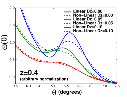
These results suggest we should measure $\theta_{BAO}$ using an alternative method to the position of the local maximum of $\omega(\theta)$. Currently, the ratio of the power spectrum to a smooth fit is used, to avoid the effect of the tilting function, which changes the peak position (Seo et al., 2008; Seo et al., 2009; Crocce & Scoccimarro, 2008; Smith et al., 2008). Here we present an alternative method based on the angular correlation function. This will be the subject of the subsequent sections.

4 Method to Recover $\mn@boldsymbol{\theta}_{\bf BAO}$

Trying to overcome the problems induced by the photo-z, we propose a new method based on an empirical parametrization of $\omega(\theta)$, which can be used even when there is no local maximum. The most important points of the method, the parametrization of $\omega(\theta)$ and the correction for the projection effect due to the width of the redshift bin are explained in detail in sections 4.1 and 4.2, respectively. The full recipe to obtain the BAO scale as a function of redshift is as follows:

1. Divide the full galaxy sample in redshift bins.

2. Compute the angular two-point correlation function in each redshift bin.

3. Parametrize the correlation function using the expression:

   $$\omega(\theta)=A+B\theta^{\gamma}+Ce^{-(\theta-\theta_{FIT})^{2}/2\sigma^{2}}$$ (7)

   and perform a fit to $\omega(\theta)$ with free parameters $A$, $B$, $C$, $\gamma$, $\theta_{FIT}$ and $\sigma$.

4. The BAO scale is estimated using the parameter $\theta_{FIT}$, and correcting it for the projection effect (see Eq. 8 below). The BAO scale as a function of the redshift is the only parameter needed to apply the standard ruler method. The cosmological interpretation of the other parameters is limited, since this is an empirical description, valid only in a neighborhood of the BAO peak, as is described in section 4.1.

5. Fit cosmological parameters to the evolution of the corrected $\theta_{BAO}$ with $z$.

4.1 Parametrization of $\mn@boldsymbol{\omega}(\mn@boldsymbol{\theta})$

Figure 2: Goodness of the parametrization for several redshifts, several bin widths and several cosmologies.

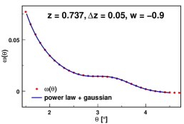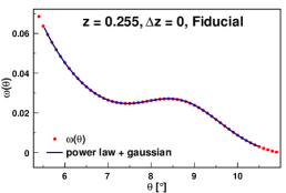
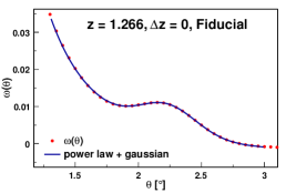
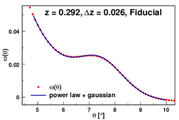
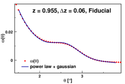
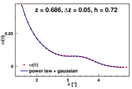
The correlation function $\omega(\theta)$ is parametrized as in Eq. (7). A power law is used to describe the shape of the correlation function before and after the peak, and a Gaussian to describe the BAO feature. The mean of the Gaussian is used to locate the BAO scale. The parameter $A$ takes into account that the correlation function can go to negative values after the BAO peak. The parameters $B$ and $C$ describe the relative weight of the two terms of the parametrization. The parameter $\gamma$ is the index of the power law, while $\theta_{FIT}$ and $\sigma$ are the mean and the width of the Gaussian, respectively.

$h$	$\Omega_{M}$	$\Omega_{b}$	$\Omega_{k}$	$w_{0}$	$w_{a}$	$n_{s}$
0.70	0.25	0.044	0.00	$-$1.00	0.0	0.95
0.68
0.72
	0.20
	0.30
		0.040
		0.048
			+0.01
			$-$0.01
				$-$0.90
				$-$1.10
					$-$0.1
					+0.1
						1.00

Table 1: Summary of the 14 cosmological models used to test the method. Where empty, the fiducial values (first line) are assumed.

We have tested the goodness of this parametrization in a redshift interval which ranges from 0.2 to 1.4, for a wide range of widths of the redshift bins (from 0 to 0.2) and for 14 cosmological models, which are listed in Table 1. The parametrization is good within 1%, i.e., the fit is good (the value of $\chi^{2}$/ndof ranges from 0.98 to 1.01, and the probabilities of the fit from 0.6 to 0.9) when the error in each point of the correlation function is $\sim 1\%$ for all bin widths and cosmological models. This precision is much better than that expected in any realistic redshift survey, since it is much smaller than the cosmic variance. Several examples of the parametrization can be seen in Fig. 2. Other functional forms have been tested, but all of them are more complex and show no improvements on the description of the data.

There is a region of stability to choose the starting and end points of the fit, which will be described in more detail in section 5.4.1. This region cannot be made arbitrarily large, since the description cannot be good for very low angles, due to non-linearities and changes in the power law index; neither for very large angles, since the correlation function changes its slope after the BAO peak.

4.2 Correcting for Projection Effects

The projection offset discussed in Sec. 3 is also present for the parametrization method. If we want to extract cosmology from this measurement, it is necessary to correct the fitted $\theta_{FIT}$ for the projection effect to recover $\theta_{BAO}$.

$$\theta_{BAO}=\alpha\,\,\theta_{FIT},$$ (8)

where $\alpha$ could in principle be a function of redshift, bin width and cosmology. However, if we want to do this correction in an unbiased way, it must be cosmology independent. We have tested the method for the 14 different cosmologies summarized in Table 1, and for different redshift bin widths.

For each of the 14 considered models, each of the considered redshifts and each of the considered bin widths, we compute the angular correlation function. We use Eq. 1 and include non-linearities (see section 2). The calculation includes also the effect of the galaxy distribution with the redshift, as descibed in section 5.2. The redshift ranges from 0.2 to 1.4 and the bin width from 0 to 0.2, as has been previously stated. We then apply the fitting method to obtain the position of the BAO peak. Two main results are obtained:

• The shift of $\theta_{FIT}$ with respect to $\theta_{BAO}$ has a universal shape, independent of the cosmology. Thus the correction function $\alpha$ depends only on redshift and bin width, but not on the cosmological model, i.e., $\alpha=\alpha(z,\Delta z)$, within a precision $<1\%$.

• After applying this universal shift, the recovered BAO scale agrees with the true value for all cosmologies to a precision of $\leq 0.75\%$. In particular, for infinitesimal bin widths, the method is able to compensate the displacement of the BAO bump due to the tilting function, correcting the 2% difference which has been observed in Sánchez et al. (2008).

These two results are presented in Figure 3, where we plot the evolution of the shift, taking the angular scale corresponding to the sound horizon scale as the reference, for 5 different redshifts, for several bin widths and for the 14 cosmological models. The spread of the results is constant with the redshift bin width, and comes from a possible residual dependence on the cosmology together with the intrinsic limitations of the method (see section 5.3 on systematic errors). The average value of this shift is the correction applied to the fitted $\theta_{FIT}$. After this correction, the true value for the BAO scale is recovered for any bin width and cosmology. Note that the absolute value of the projection effect changes with the cosmological model, since both the BAO position and the radial distance change. However, the relative effect is cosmology independent, as shown in Figure 3.

Figure 3: Evolution of the shift of the measured $\theta_{FIT}$ with the width of the redshift bin for the 14 cosmological models considered in this work. The sound horizon scale $\theta_{BAO}$ for each cosmological model is taken as the reference. Two results are obtained. First, the correct sound horizon scale is recovered for any cosmological model within 0.75% for infinitesimal redshift shells. Second, the shape of the shift is universal, and the spread is constant with the redshift bin width. Note that the dispersion between models is much smaller ($\leq 1\%$) than the shift due to increasing binwidth. At low redshifts, $z<0.3$, the shift can be $\sim 15$% for $\Delta z\geq 0.1$, while at high redshifts, $z>0.5$, the shift saturates at around 7%.

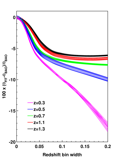
As has already been noted (Simpson et al., 2009), the projection effect is much more pronounced at low redshift. This must be taken into account to choose the optimum size of the redshift bins. The correction must be kept as small as possible, given the limitations imposed by the photo-z precision, to introduce small systematic uncertainties. We are using a Gaussian form for the photo-z uncertainty, because if the requirements on photo-z measurement for a survey like DES are fulfilled, the effects of a possible non-Gaussianity are kept small. If this is not the case, the evaluation of the true width of the bin must be refined. This is another reason to maintain the correction small.

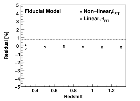
Note that the BAO scale is recovered both for linear and non-linear theory for infinitesinal bin width. This can be seen in Figure 4, where the residual of the fit with respect to the theoretical $\theta_{BAO}$ as a function of redshift is shown for the fiducial cosmological model. The recovered values are well inside the 0.75% precision that we quote as systematic error, represented by the dotted lines. This happens for all the cosmological models, showing that the method is robust and able to recover the theoretical BAO scale.

Figure 4: Residual of the result of the parametric fit $\theta_{FIT}$ with respect to the the theoretical value of the BAO scale as a function of redshift for the fiducial model. The open dots show the results obtained from the fit to the linear correlation functions and the solid dots show the results on the non-linear correlation functions. In both cases the theoretical values are recovered, well inside the quoted systematic error of 0.75%, shown by the dotted lines.

4.3 Redshift Space Distortions

There are other effects which are important in order to have under control the parametric description of the angular correlation function. In particular, redshift space distortions must be taken into account in the analysis of the BAO scale, since they result in an anisotropic correlation function. We need to replace $\xi(r)$ in Eq. 1 by $\xi(\sigma,\pi)$ with $\pi=\chi_{2}-\chi_{1}$, the radial separation, and $\sigma^{2}=2\chi_{1}\chi_{2}(1-\cos{\theta})$, the perpendicular separation. Galaxy pairs separated by large radial distances infall into each other which means that they are measured as contributing to bins of smaller radial separation (in redshift space) than in real (or true) space. This results in larger correlations (more pairs) at intermediate scales ($\pi<20$ Mpc/h) and lower correlation at larger separations. The redshift space correlation becomes negative for $\pi>40$ Mpc/h while the real space correlation remains positive until $\pi>130$ Mpc/h (see Fig. A1 in Gaztañaga et al. 2009). Recall from Eq. 1 how the angular correlation is just a mean over the radial distance within the corresponding redshift bin. This means that for narrow redshift bins (of width comparable to $\pi\simeq 100$ Mpc/h) the resulting angular correlation can be quite different in real and redshift space (Fisher et al., 1995; Padmanabhan et al., 2007; Nock et al., 2010). As the total number of pairs is conserved, the integral over all separations is the same in real and redshift space, so that one expect to find the same angular correlation only for broad redshift bins, where the contribution of the boundary to the integral is negligible.

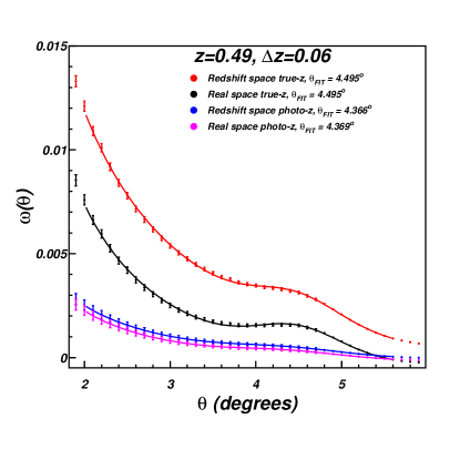
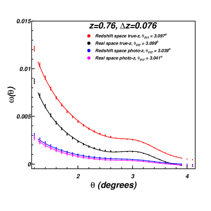
The resulting predictions for redshift space agree very well with MICE simulations (more details can be found in Crocce et al. 2010). Fig. 5 shows some examples of this redshift space modeling for linear theory for two of the redshift bins used in the analysis presented above. Symbols (with 2% nominal errors) correspond to the linear model predictions when we include the redshift space distortions as well as photo-z distortions. Note how both redshift space and photo-z distortions change quite dramatically the amplitude of the resulting angular correlation.

The lines in Fig. 5 show the results of a fit of our parametrization (in Eq. 7) to these new predictions. The corresponding fit values of $\theta_{FIT}$ are shown in the label. As expected, there is a small but systematic shift of $\theta_{FIT}$ to smaller angles in the case of photo-z distortions. This is because the effetive redshift bin is wider due to the photo-z errors. This effect is taken into account by the correction shown in Fig. 3 (once we use the equivalent width of the true redshift distribution). Crocce et al. (2010) shows that the model we are using to predict the errors also works in redshift space.

As can be seen in Fig. 5, the parametrization absorbs very well the effects of redshift space distortions and the value recovered for $\theta_{FIT}$ agree well in real and redshift space despite the large difference in amplitude. This is not too surprising as we have already shown above that this parametrization works for different cosmological models, different redshifts and also different redshift widths.

Figure 5: Effect of z-distortions and photo-z. Points (with nominal 2% errors) show the linear theory prediction, while lines correspond to a fit to our parametrization in Eq. 7. Labels indicate the corresponding values of $\theta_{FIT}$ in each case.

5 Application to the Dark Energy Survey

5.1 The Dark Energy Survey

The Dark Energy Survey (DES)  is a next generation sky survey aimed directly at understanding the nature of the dark energy. It will use 30% of the available time on the Blanco telescope at CTIO, during 5 years. The survey is designed to produce photometric redshifts in the range $0.2<z<1.4$, and will cover 5000 square degrees in the southern hemisphere. The filters to be used are $g$, $r$, $i$, $z$, $Y$.

DES has been designed to exploit mainly 4 methods in order to study the dark energy. These methods are the galaxy cluster counting and spatial distribution of galaxy clusters, the shifting of the galaxy spatial angular power spectra with redshift, weak gravitational lensing measurements on several redshift shells, and distances to $\sim 2000$ supernovae. Using these techniques, a 5%-15% precision measurement in the equation of state parameter $w$ from each of our methods, and a 30% measurement in the variation of $w$ with time are expected. Combined, they provide both stronger constraints and a check on systematic errors.

5.2 N-body Simulation Features

We have developed and tested our method to recover the angular scale of the sound horizon using a large N-body simulation capable of reproducing the geometry (e.g. area, density and depth) and specifications of DES .

The simulated data was kindly provided by the MICE project team, and consisted of a distribution of dark matter particles (galaxies, from now on) with the cosmological parameters fixed to the fiducial model of Table 1. The radial profile matches the DES expectation

$$dN/dz\propto(z/0.5)^{2}\exp{-(z/0.5)^{1.5}},$$ (9)

the simulation covers $1/8$ of sky ($\sim 5000$ square degrees) in the redshift range $0.2<z<1.4$, containing 50 million galaxies. All these numbers roughly match the DES expectations for the main galaxies. These data was obtained from the comoving output at $z=0$ of one of the largest N-body simulations completed to date, with comoving size $L_{box}=3072\,{\it h}^{-1}\,{\rm Mpc}$ and more than $8\times 10^{9}$ particles ($m_{p}=2.3\times 10^{11}\,{\it h}^{-1}\,M_{\odot}$). More details about this run can be found in Fosalba et al. (2008) and Crocce et al. (2009).

Figure 6: Photo-z precision used in this analysis (continuous line), as compare to used bins position and width (dots).

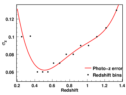
The precision in the determination of the redshift for galaxies which has been used in this analysis is shown in Figure 6. This is the typical precision that is obtained using the current photo-z codes for DES (Banerji et al., 2008). This photo-z has been introduced into the simulation, to produce a catalog of galaxies similar to that expected in DES, where the proposed procedure to recover $\theta_{BAO}$ has been applied. The photo-z has been introduced by scattering each individual redshift according to the Gaussian representing the photo-z error of Figure 6. The redshift bin widths have been chosen as a compromise between statistics, expected precision in the photo-z determination and shift of the BAO peak due to projection effect. Then, the redshift bins used in this analysis follow the expected precision in the photo-z measurement, being wider for low and high redshifts and narrower for mid redshift. The analysis is performed in the full redshift range, from $z=0.2$ to $z=1.4$. With this prescription we have 14 bins, represented also as dots in Figure 6. The position of the dot in the horizontal axis represents the bin center, and the position in the vertical axis represents the bin width, which has been chosen to be close to the expected $1-\sigma$ error in photo-z measurement. Much wider bins make the sensitivity too small due to projection effect (the amplitude of the correlation function becomes very small and the shift of the peak becames very large), while much narrower bins make the correlations between redshift bins too large, complicating the analysis and also diminishing the sensitivity.

5.3 Results

Figure 7: Correlation functions for MICE simulation, including photo-z effects. The errors are computed using Eq 12.

In order to numerically estimate the angular correlation function in a given redshift bin, we have used the Landy-Szalay estimator (Landy & Szalay, 1993). The random catalogs contain as many galaxies as the simulation, since the shot noise error is negligible, given the size of the sample.

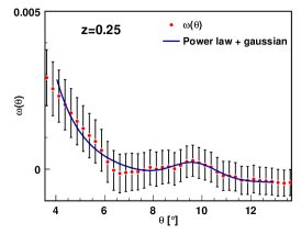
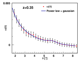
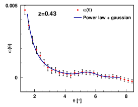
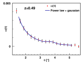
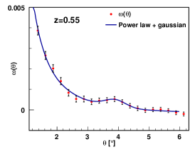
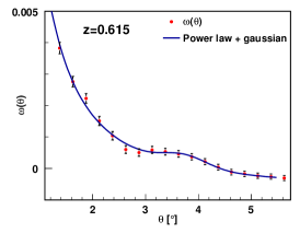
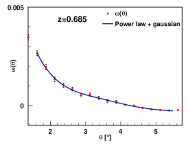
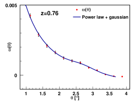
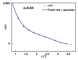
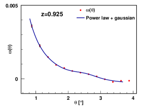
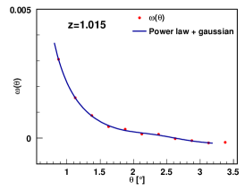
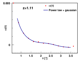
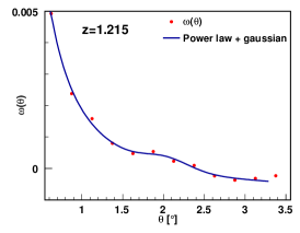
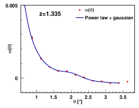
The resulting correlation functions together with their parametrizations are presented in Fig. 7. The statistical error in $\theta_{FIT}$ is given as the error in the fit coming from the error in the correlation function, as explained in section 2, and taking into account the photo-z effect, as described in Eq. 12 below.

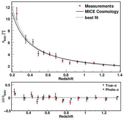
The recovered values of $\theta_{BAO}$ after applying the correction of Eq. 8 can be seen in Fig. 8 (top) as a function of the redshift. The correction is applied after evaluating the true width of the redshift bin, using $\Delta z_{true}=\sqrt{2\pi}\Delta z_{photo}$, which corresponds to the width of a top-hat bin in true-z which gives the same amplitude in $\omega(\theta)$ than the chosen photo-z bin. The points include also the systematic errors, described in section 5.4. The MICE cosmology is also shown as the solid line, and the best fit cosmology as the dashed line. To compare, the same analysis has been applied to the true redshifts catalog (i.e., without photo-z). The corresponding result is presented in the bottom panel of Figure 8, together with the photo-z. The results obtained using the true redshift are closer to the MICE cosmology, as expected. For true redshifts, the bin width is not corrected, and the systematic errors do not include any photo-z contribution.

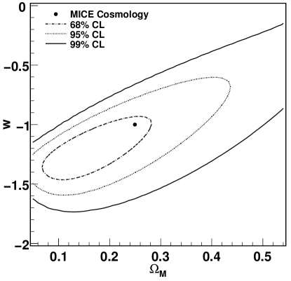
The true cosmology is recovered after applying the analysis method, both for the photo-z results and for the true z results. The photo-z result is shown in Fig. 9, where the MICE cosmology is inside the 1-$\sigma$ contours. These contours have been obtained fitting the cosmology to the results presented in Fig. 8 (top), with free parameters $\Omega_{M}$ and $w$, and fixing all the other parameters to their MICE values.

In order to perform this fit, we need to take into account the correlation between bins induced by photo-z. To do this, we compute the migration matrix $r_{ij}$, given by the probability that a given galaxy at bin $i$ is measured at bin $j$ due to the photo-z error. Once the migration matrix is computed (just counting the number of galaxies that migrate from bin $i$ to bin $j$ in the simulation), the calculation of the covariance matrix $C_{ij}$ is straightforward. Since

$$N_{i}^{O}=\sum_{j=1}^{N_{bins}}r_{ij}N_{j}^{T}$$ (10)

where $N_{i}^{O}$ is the number of observed galaxies in bin $i$, $r_{ij}$ is the migration matrix and $N_{j}^{T}$ is the true number of galaxies in bin $j$, then the observed and true correlation functions are related by (Benjamin et al., 2010):

$$w_{i}^{O}(\theta)=\sum_{k=1}^{N_{bins}}r_{ik}^{2}\frac{(N_{k}^{T})^{2}}{(N_{i}^{O})^{2}}w_{k}^{T}(\theta)$$ (11)

where $w_{i}^{O}(\theta)$ is the observed correlation function in bin $i$ at scale $\theta$ and $w_{i}^{T}(\theta)$ is the true correlation function in bin $i$ at scale $\theta$, given by Eq. 1. Then, the covariance for the correlation functions can be written

$$C_{ij}=\langle\Delta w^{O}_{i}(\theta)\Delta w^{O}_{j}(\theta^{\prime})\rangle=\sum_{k=1}^{N_{bins}}(r_{ik}^{2}r_{jk}^{2})\frac{(N_{k}^{T})^{4}}{(N_{i}^{O})^{2}(N_{j}^{O})^{2}}{\rm Cov}_{\theta\theta^{\prime}}$$ (12)

where ${\rm Cov}_{\theta\theta^{\prime}}$ is given in Eq. 6. This expression neglects the intrinsic correlations between bins. Whether this is a good approximation depends mainly on the bin widths. In our case, adjacent bin centers are separated by more than 200 Mpc/$h$, and we find that the intrinsic cross-correlations can be safely ignored. Thus, with photo-z errors, the observed correlation functions and covariances are given by Eqs.  11 and  12, respectively, rather than Eqs. 1 and  6.

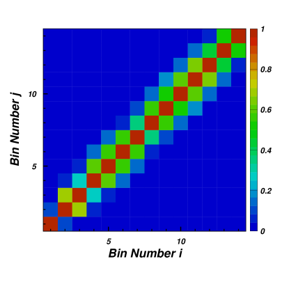
The resulting correlation coefficients, computed from $C_{ij}$, for redshift bins are depicted in Figure 10. The induced correlation extends to 3 bins. This correlation matrix is converted to the covariance of $\theta_{BAO}$ angles, $\widehat{C}_{ij}$, including the corresponding errors.

Therefore, we use the $\widehat{C}_{ij}$ to compute the $\chi^{2}$ for the fit in the usual way:

$$\chi^{2}(\Omega_{M},w)=\sum_{i,j}^{N_{bins}}(\widehat{\theta}^{i}_{BAO}-\theta^{i}_{BAO})\widehat{C}^{-1}_{ij}(\widehat{\theta}^{j}_{BAO}-\theta^{j}_{BAO})$$ (13)

where $\theta^{i}_{BAO}$ is the angular scale corresponding to the sound horizon for cosmological parameters $\Omega_{M},w$ at the redshift of bin $i$, and $\widehat{\theta}^{i}_{BAO}=\alpha\,\,\theta_{FIT}$ is the measured angle in bin $i$. All the results include the systematic errors in the measurements of $\widehat{\theta}_{BAO}$, described more in detail in the next section. The statistical error is correlated using the computed covariance matrix. Some of the systematic errors (coming from photo-z and redshift space distortions) are also correlated, while the others are uncorrelated and are just added in cuadrature to the diagonal of the covariance matrix. All these numbers match the DES requirements. The total area of the survey, together with the magnitude limits, which fix the galaxy density, contribute to the errors on $\omega(\theta)$. Moreover, the photo-z requirements fix the level of correlation among redshift bins.

If we restrict to a one-dimensional analysis, and fix $\Omega_{M}=0.25$, then we obtain for the equation of state of the dark energy $w=-1.05\pm 0.14$. The precision on this result depends on the photo-z error, which is the dominant source of systematic uncertainties. If the photo-z error is decreased, the precision in $w$ correspondingly improves. For a more optimistic estimation of $\Delta z\sim 0.03(1+z)$ it becomes $\Delta w\sim 0.10$.

Figure 8: Evolution of the measured $\theta_{BAO}$ with the redshift (top). Comparison of the results obtained using photo-z and the true-z (bottom). The true-z results are closer to the MICE cosmology, as expected.

Figure 9: Allowed region for the cosmological parameters at 68 (dashed-dotted line), 95 (dashed line) and 99 (solid line) % C. L. The true cosmology, given by the dot, is recovered within 1-$\sigma$ .

Figure 10: Correlation matrix for redshift bins. The correlation extends to 3 bins, and is taken into account in the fit of the cosmological parameters.

5.4 Systematic Errors

We have identified several sources of systematic errors for this methodology:

• Uncertainties in the fitting procedure (method error).

• Residual errors due to the correction in $\theta_{FIT}$ coming from a possible residual dependence on the cosmological model (cosmology independence).

• Uncertainties in the theory coming from the implementation of non-linearities (modeling error).

• Effects of the redshift space distortions on the BAO scale (z-distortions error).

• Uncertainty in the redshift determination (photo-z error).

A brief quantitative summary of these effects is given in Table 2, that follows from the different analysis discussed below.

Systematic error	$\Delta\theta_{BAO}$	Correlated between bins
Parametrization	1.0%	No
Photometric redshift	5.0%	Yes
Redshift space distortions	1.0%	Yes
Theory	1.0%	No
Projection effect	1.0%	No

Table 2: Estimation of various systematic errors. Some of them are correlated between redshift bins (photo-z and z-distorions errors). The others are not.

5.4.1 Method Error

To compute the systematic error associated to the parametrization method, we have done some further analysis on theoretical angular correlation functions with the same bin widths and central redshifts as those used in the analysis of the MICE simulation. The error associated to the method comes from the possible influence in the obtained $\theta_{FIT}$ of the range of angles used to perform the fit. To evaluate the error, we have varied this range for all 14 z-bins we have, and performed the fit for each range.

Figure 11: $\theta_{BAO}$ dispersion as a function of the starting and end point of the fitted region. Only two bins are shown, where the maximum of the effect is observed, at redshifts 0.43 (top) and 1.015 (bottom). All the bins behave in a very similar way, but with smaller variations. The observed variation in the results is slightly smaller than 1%, and a conservative 1% systematic error is associated to the fit method.

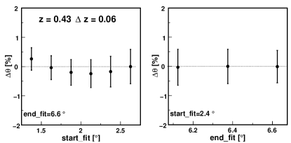
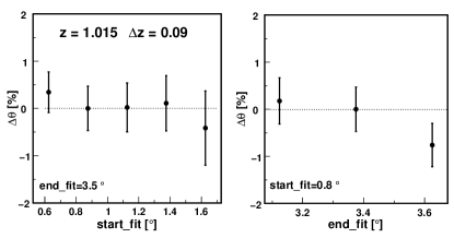
In the decision of the range to be fitted, we have to choose a starting point at angles smaller than the BAO peak and an end point after the peak. By varying this two angles we can study how much the result vary with this decision. Results can be seen in Fig. 11, where the obtained $\theta_{FIT}$ is shown for different starting points and end points of the fit, for low and high redshift. These results show the bins where the maximum differences are observed. In all cases, the uncertainty is always of the order of, but slightly below, 1%. We have conservatively assigned a 1% systematic error associated to the method, since this error is subdominant.

5.4.2 Cosmology Independence

The dispersion of all the cosmological models around a common value for the projection effect correction is small, $\leq 1\%$, as can be seen in Figure 3. This dispersion propagates directly to the corrected $\theta_{FIT}$ as a source of uncertainty. Conservatively, we have asigned a systematic error of 1% associated to the independence of the cosmology.

5.4.3 Modelling Error

Also the error due to the uncertainty in the theory (non-linearities at the scale of the BAO peak) has been computed obtaining a global error of 1%, estimated in a conservative way as the difference between the $\theta_{FIT}$ measured using linear and non-linear $\omega(\theta)$, for the same redshift bins of the analysis. The difference for infinitesimal bins is presented in Fig. 4.

5.4.4 Photo-z Error

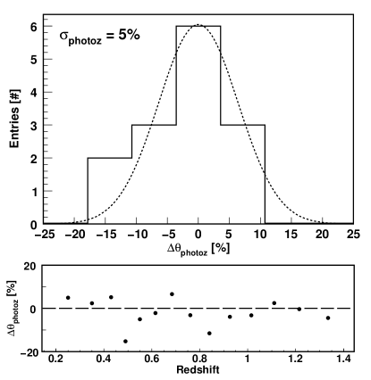
To compute the systematic error associated to photo-z measurement, we have analysed the simulation using the true redshifts in the same way we do for the photo-z. We can estimate the deviation in $\theta_{FIT}$ due to photo-z errors computing the difference between the result obtained using the catalog with true-z and the result obtained using the catalog with photo-z. In Fig. 12 (top) we can see the distribution of those differences. Photo-z uncertainties do not introduce a significant bias, but they do introduce a dispersion around the central value. This dispersion is around 5%, which we assign as the systematic error coming from the photometric error. We are assuming here that this error is redshift independent, which given the scope of the current analysis is reasonable, as shown in Fig. 12 (bottom). The differences between the results of the analysis using photo-z and true z are shown as a function of the redshift, and there is no indication of any redshift dependence. This estimation could be further refined by using many simulations and repeating this study for each redshift bin as many times as simulations we use. This is out of the scope of this work, where we can only indicate the order of magnitude of the systematic errors, but should be done for a real survey, since this will be the dominant source of systematic uncertainty.

Figure 12: Cumulated Difference between the measured $\theta_{FIT}$ in the photo-z catalog and the true z catalog for the 14 bins of the analysis (top). The dispersion is 5%, that we use as the systematic error. This error is taken as constant with redshift, since there is no clear dependence when the differences are plotted as a function of redshift (bottom).

5.4.5 Other Systematic Errors

There are some other potential systematic errors, like those arising from the uncertainty in the description of the redshift space distortions, the gravitational lensing magnification or those mainly associated to the used galaxy sample, as the bias of the population.

The uncertainties in the description of the redshift space distortions can induce a systematic error in the determination of the sound horizon scale. To evaluate it, we have changed the parameters of the z-distortions within their uncertainties, finding a value of $\Delta\theta_{BAO}\sim 0.5-1\%$, in good agrreement with the effect seen in Fig. 5.

At the BAO scales it is a good approximation to consider that the bias is scale independent (Cresswell & Percival, 2009; Crocce et al., 2010), and given the width of the redshift bins, we can safely use a redshift independent bias inside each one. The redshift dependence of bias may appear in a different normalization of the correlation function between different redshift bins. Since we do not care about the overall normalization and only about the position of the peak, we are not sensitive to $b(z)$. We have tested that the change in overal amplitude of the correlation function does not affect to our determination of the sound horizon scale, even if the error in the correlation function is changed. Moreover, we have tested the effect of a scale dependent bias, introducing artificially the effect in the correlation functions, using an approximated Q-model with the determination of parameters of Cresswell & Percival (2009). The bias variation with $\theta$ in the fit region of $\omega(\theta)$ ranges from 1% to 6%, and induces a change in the determination of the sound horizon scale below 1%, well within statistical uncertainties.

Finally, the gravitational lensing magnification can affect the $\omega(\theta)$ (Loverde et al., 2008) introducing correlations between bins at different redshifts. However, the effect of the magnification is concentrated at very low angles, and the magnitude of the induced correlation is much smaller than the correlation induced by photo-z, which has already been studied and used in this analysis. Therefore, the position of the BAO peak is free of systematics coming from magnification. Consequently, all this effect is not considered here.

6 Conclusions

We have developed a new method to measure the BAO scale in the angular two-point correlation function. This method is adapted to photometric redshift surveys, where the information along the line of sight is lost due to the photo-z precision, and only the angular information survives, although it can be applied to any survey. Two main results are found. First, the sound horizon scale can be recovered from the non-linear angular correlation functions to a precision $\leq$0.75% applying the parametric fit described in the text, for any cosmological model for infinitesimal redshift shells (i.e. for the 3D correlation function). This is not totally surprising. It can be understood if we approximate the 3D linear correlation as a sum of a BAO gaussian and a baseline that is well described by a power-law. If we neglect mode coupling effects, the non-linear correlation is given by a convolution with a gaussian damping, which leave unchanged the Gaussian position. Under this assumption our parametric fit should be able to recover the true BAO positions without any bias. Second, the shift of the BAO peak due to projection effects has a universal shape, does not depend on the cosmological model, and only depends on the redshift and the redshift bin width. This can be used to correct the result obtained for wide photo-z bins and recover the true sound horizon scale. The method has been tested with a mock catalog built upon a large N-body simulation provided by the MICE collaboration, with characteristics similar to those expected in DES. The true cosmology is recovered within 1-$\sigma$. The correlation between redshift bins and a preliminary evaluation of the systematic errors have been included in this study, and we find that the most important systematic error arises from the photo-z precision. The method is very promising and very robust against systematic uncertainties.

Note that our analysis over the MICE simulations was in real, rather than in redshift space. Over a comoving output, rather than over an evolving distribution. Over dark matter particles, instead of galaxies. We believe that all this simplifications are not essential limitations to the method presented here, as we have shown that both the modeling and the error analysis are quite generic and work in real, redshift and photo-z space. If anything, redshift space distortions (and possibly biasing) produce larger amplitudes, in which case our results are conservative in the sense that more realistic simulations (or observations) will produce smaller error bars than the ones presented here.

References

- Banerji et al. (2008) Banerji M., Abdalla F. B., Lahav O., Lin H., 2008, MNRAS, 386, 1219
- Benítez et al. (2009) Benítez N., et al., 2009, ApJ, 691, 241
- Benjamin et al. (2010) Benjamin J., Van Waerbeke L., Menard B., Kilbinger M., 2010, arXiv: 1002.2266 [astro-ph]
- Bharadwaj (1996) Bharadwaj S., 1996, ApJ, 472, 1
- Cabre et al. (2007) Cabre A., Fosalba P., Gaztanaga E., Manera M., 2007, arXiv: astro-ph/0701393
- Colless et al. (2001) Colless M., et al., 2001, MNRAS, 328, 1039
- Cresswell & Percival (2009) Cresswell J. G., Percival W. J., 2009, MNRAS, 392, 682
- Crocce et al. (2010) Crocce M., Cabré A., Gaztañaga E., 2010, arXiv:1004.4640 [astro-ph]
- Crocce et al. (2009) Crocce M., Fosalba P., Castander F. J., Gaztanaga E., 2009, arXiv: 0907.0019 [astro-ph]
- Crocce & Scoccimarro (2006) Crocce M., Scoccimarro R., 2006, PRD, 73, 063519
- Crocce & Scoccimarro (2008) Crocce M., Scoccimarro R., 2008, PRD, 77, 023533
- Eisenstein et al. (2005) Eisenstein D. J., et al., 2005, ApJ, 633, 560
- Eisenstein et al. (2007) Eisenstein D. J., Seo H., White M., 2007, ApJ, 664, 660
- Fisher et al. (1995) Fisher K. B., Lahav O., Hoffman Y., Lynden-Bell D., Zaroubi S., 1995, MNRAS, 272, 885
- Fosalba et al. (2008) Fosalba P., Gaztañaga E., Castander F. J., Manera M., 2008, MNRAS, 391, 435
- Gaztañaga et al. (2009) Gaztañaga E., Cabré A., Hui L., 2009, MNRAS, 399, 1663
- Hütsi (2006a) Hütsi G., 2006a, A&A, 449, 891
- Hütsi (2006b) Hütsi G., 2006b, A&A, 459, 375
- Ilbert et al. (2006) Ilbert O., et al., 2006, A&A, 457, 841
- Kaiser et al. (2000) Kaiser N., Tonry J. L., Luppino G. A., 2000, PASP, 112, 768
- Komatsu et al. (2010) Komatsu E., et al., 2010, arXiv:1001.4538 [astro-ph]
- Landy & Szalay (1993) Landy S. D., Szalay A. S., 1993, ApJ, 412, 64
- Loverde et al. (2008) Loverde M., Hui L., Gaztañaga E., 2008, PRD, 77, 023512
- Matsubara (2008) Matsubara T., 2008, PRD, 77, 063530
- Matsubara et al. (2004) Matsubara T., Szalay A. S., Pope A. C., 2004, ApJ, 606, 1
- Nock et al. (2010) Nock K., Percival W. J., Ross A. J., 2010, arXiv: 1003.0896 [astro-ph]
- Okumura et al. (2008) Okumura T., Matsubara T., Eisenstein D. J., Kayo I., Hikage C., Szalay A. S., Schneider D. P., 2008, ApJ, 676, 889
- Padmanabhan et al. (2007) Padmanabhan N., et al., 2007, MNRAS, 378, 852
- Padmanabhan & White (2009) Padmanabhan N., White M., 2009, PRD, 80, 063508
- Peebles (1980) Peebles P. J. E., 1980, The large-scale structure of the universe
- Percival et al. (2007) Percival W. J., Cole S., Eisenstein D. J., Nichol R. C., Peacock J. A., Pope A. C., Szalay A. S., 2007, MNRAS, 381, 1053
- Rassat et al. (2008) Rassat A., et al., 2008, arXiv: 0810.0003 [astro-ph]
- Sánchez et al. (2008) Sánchez A. G., Baugh C. M., Angulo R., 2008, MNRAS, 390, 1470
- Sánchez et al. (2009) Sánchez A. G., Crocce M., Cabré A., Baugh C. M., Gaztañaga E., 2009, MNRAS, 400, 1643
- Seo et al. (2009) Seo H., Eckel J., Eisenstein D. J., Mehta K., Metchnik M., Padmanabhan N., Pinto P., Takahashi R., White M., Xu X., 2009, arXiv:0910.5005 [astro-ph]
- Seo & Eisenstein (2007) Seo H., Eisenstein D. J., 2007, ApJ, 665, 14
- Seo et al. (2008) Seo H., Siegel E. R., Eisenstein D. J., White M., 2008, ApJ, 686, 13
- Simpson et al. (2009) Simpson F., Peacock J. A., Simon P., 2009, PRD, 79, 063508
- Smith et al. (2008) Smith R. E., Scoccimarro R., Sheth R. K., 2008, PRD, 77, 043525
- The Dark Energy Survey Collaboration (2005) The Dark Energy Survey Collaboration 2005, arXiv:astro-ph/0510346
- Tyson et al. (2003) Tyson J. A., Wittman D. M., Hennawi J. F., Spergel D. N., 2003, Nuclear Physics B Proceedings Supplements, 124, 21
- York et al. (2000) York D. G., et al., 2000, AJ, 120, 1579