Agent dynamics in kinetic models of wealth exchange

Abstract

We study the dynamics of individual agents in some kinetic models of wealth exchange, particularly, the models with savings. For the model with uniform savings, agents perform simple random walks in the “wealth space”. On the other hand, we observe ballistic diffusion in the model with distributed savings. There is an associated skewness in the gain-loss distribution which explains the steady state behavior in such models. We find that in general an agent gains while interacting with an agent with a larger saving propensity.

I Introduction

The distribution of wealth among individuals in an economy has been a very important area of research in economics, for more than a century Pareto:1897 ; Mandelbrot:1960 ; EWD05 ; ESTP ; SCCC ; Yakovenko:RMP . The same holds for income distribution in any society. Detailed analysis of the income distribution EWD05 ; ESTP ; SCCC so far indicate that for large income $m$,

$$P(m)\sim m^{-(1+\nu)},$$ (1)

where $P$ denotes the number density of people with income or wealth $m$. The power law in income and wealth distribution is named after Pareto and the exponent $\nu$ is called the Pareto exponent. The tail of the income distribution indeed follows the above mentioned behavior and the value of the Pareto exponent $\nu$ is generally seen to vary between 1 and 3 EWD05 ; SCCC ; Yakovenko:RMP ; datapap . For any country, it is well known that typically less than $10\%$ of the population possesses about $40\%$ of the total wealth and they follow the above law, while the rest of the low income population, follow a different distribution EWD05 ; SCCC ; Yakovenko:RMP ; datapap ; marjitIspolatov ; Dragulescu:2000 .

According to physicists, the regular patterns observed in the income (and wealth) distribution are indicative of a natural law for the statistical properties of a many-body dynamical system representing the entire set of economic interactions in a society, analogous to those previously derived for gases and liquids. By viewing the economy as a thermodynamic system, one can identify the income distribution with the distribution of energy among the particles in a gas. This has led to several new attempts at explaining them, particularly, a class of kinetic exchange models have provided a simple mechanism for understanding the unequal accumulation of assets. These models are simple from the perspective of economics and implement the key factors in socioeconomic interactions that results in very different societies converging to similar forms of unequal distribution of resources (see Refs. EWD05 ; ESTP , for a collection of large number of technical papers in this field).

In this paper, we consider the dynamics of individual agents. We discuss the money distribution of agents, given a particular value of saving propensity. In models with distributed savings, we look at a tagged agent, and compute the distribution of money gained or lost in each interaction. We project the gain-loss behavior into a walk in one dimension in a so called “wealth space”. Our numerical simulations suggest evidence of ballistic diffusion.

II Gas-like models

In analogy to two-particle collision process which results in a change in their individual kinetic energy or momenta, income exchange models may be defined using two-agent interactions: two randomly selected agents exchange money by some pre-defined mechanism. The exchange process does not depend on previous exchanges, hence it is a Markov process:

$$\left(\begin{array}[]{c}m_{i}(t+1)\\ m_{j}(t+1)\end{array}\right)={\mathcal{M}}\left(\begin{array}[]{c}m_{i}(t)\\ m_{j}(t)\end{array}\right)$$ (2)

where $m_{i}(t)$ is the income of agent $i$ at time $t$ and the collision matrix ${\mathcal{M}}$ defines the exchange mechanism.

In this class of models, one considers a system with $N$ agents (individuals or corporates) and total money $M$. This is a closed economic system where $N$ and $M$ are fixed (microcanonical ensemble), which corresponds to no migration or production in the system where the only economic activity is confined to trading. Another way of looking at this is to consider slow rates of growth or decay. Thus the microscopic time scale (of trading) is much smaller in comparison to the time scale at which the economy experiences growth or collapse.

In any trading, a pair of traders $i$ and $j$ exchange their money marjitIspolatov ; Dragulescu:2000 ; Chakraborti:2000 ; Chatterjee:rev ; Chakrabarti:2010 , locally conserve it, while nobody ends up with negative money ($m_{i}(t)\geq 0$, i.e, debt not allowed):

$$m_{i}(t+1)=m_{i}(t)+\Delta m;\ m_{j}(t+1)=m_{j}(t)-\Delta m.$$ (3)

Time ($t$) changes by one unit after each trading.

The simplest case (DY model hereafter) considers a random fraction of total money to be shared Dragulescu:2000 . The steady-state ($t\rightarrow\infty$) money follows a Gibbs distribution: $P(m)=(1/T)\exp(-m/T)$; $T=M/N$. This result is robust and is independent of the topology of the (undirected) exchange space, be it regular lattice, fractal or small-world Chatterjee:rev .

Savings is an important ingredient in a trading process Samuelson:1980 . A saving propensity factor $\lambda$ was introduced in the random exchange model Chakraborti:2000 , where each trader at time $t$ saves a fraction $\lambda$ of its money $m_{i}(t)$ and trades randomly with the rest:

$$m_{i}(t+1)=\lambda m_{i}(t)+\epsilon_{ij}\left[(1-\lambda)(m_{i}(t)+m_{j}(t))\right],$$ (4)

$$m_{j}(t+1)=\lambda m_{j}(t)+(1-\epsilon_{ij})\left[(1-\lambda)(m_{i}(t)+m_{j}(t))\right],$$ (5)

$\epsilon_{ij}$ being a random fraction, coming from the stochastic nature of the trading.

In this model (CC model hereafter), the steady state distribution $P(m)$ of money is decaying on both sides with the most-probable money per agent shifting away from $m=0$ (for $\lambda=0$) to $M/N$ as $\lambda\to 1$  Chakraborti:2000 . This model has been argued to resemble a Gamma distribution Patriarca:2004 ; Repetowicz:2005 ; Lallouache:2010 , while the exact form of the distribution for this model is still unknown. A very similar model was proposed by Angle Angle several years back in sociology journals, the numerical simulations of which fit well to Gamma distributions.

In a real society or economy, saving $\lambda$ is very inhomogeneous. The evolution of money in a corresponding model (CCM model hereafter) can be written as Chatterjee:2004 :

$$m_{i}(t+1)=\lambda_{i}m_{i}(t)+\epsilon_{ij}\left[(1-\lambda_{i})m_{i}(t)+(1-\lambda_{j})m_{j}(t)\right],$$ (6)

$$m_{j}(t+1)=\lambda_{j}m_{j}(t)+(1-\epsilon_{ij})\left[(1-\lambda_{i})m_{i}(t)+(1-\lambda_{j})m_{j}(t)\right].$$ (7)

It looks similar to the CC model, except that $\lambda_{i}$ and $\lambda_{j}$, the saving propensities of agents $i$ and $j$, are different. The agents have saving propensities, distributed randomly and independently as $\Lambda(\lambda)$, such that $\Lambda(\lambda)$ is non-vanishing as $\lambda\to 1$; $\lambda_{i}$ is quenched for each agent ($\lambda_{i}$ are independent of trading or $t$). The actual asset distribution $P(m)$ in such a model depends on the form of $\Lambda(\lambda)$, but for all of them the asymptotic form of the distribution will become Pareto-like (Eqn. (1)). For uniform distribution, $\Lambda(\lambda)=1$, $\nu=1$. However, for distributions

$$\Lambda(\lambda)\propto(1-\lambda)^{\delta},$$ (8)

$P(m)\sim m^{-(2+\delta)}$ Chatterjee:2004 ; Mohanty:2006 ; Chatterjee:rev . In the CCM model, agents with higher saving propensity tend to hold higher average wealth, which is justified by the fact that the saving propensity in the rich population is always high Dynan:2004 . Analytical understanding of CCM model has been possible until now under certain approximations Chatterjee:2005 , and mean-field theory Mohanty:2006 ; Kargupta suggests that the agent with saving $\lambda$ possesses wealth $m(\lambda)$ in the steady state, where

$$m(\lambda)=C/(1-\lambda),$$ (9)

with $C\propto 1/\log(N)$. The precise analytical formulation of the above models have been recently considered with success, and the results have been derived in most cases Toscani . There have been recent efforts in analyzing the CCM model at a microscopic scale Chatterjee:2010 . Variations of these models have been considered in several manners to obtain similar (e.g., for annealed case ecoanneal ) or different (as on networks) results Chatterjee:2009 ; Chakraborty:2010 . It has also been shown that the results are invariant even if one considers a cononical ensemble Basu:2008 . Some microeconomic formulations have also proved to be useful ChakrabartiASBK .

III Studying dynamics of agents

In the DY and CC models, agents are homogeneous. DY model is nothing but a special case of the CC model where $\lambda=0$. In these models, looking at individual agents and the whole system are equivalent. On the contrary, the presence of the distributed saving propensity (quenched disorder) in CCM model gives it a rich structure and calls for a careful look at the local scale (at the level of individuals) besides computing global quantities.

Figure 1: Distribution $P(m_{k}|\lambda_{k})$ of money $m_{k}$ for the tagged agent $k$ with a particular value of savings $\lambda_{k}$ in the CCM model with uniformly distributed savings ($\delta=0$). The data is shown for a system of $N=256$ agents.

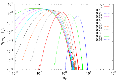
In this study, we perform extensive numerical simulations with system of $N$ agents, with uniform distribution $\Lambda(\lambda)=1$, bounded above by $1-1/N$. We look at the dynamics of a tagged agent $k$, having a saving propensity $\lambda_{k}$, in a pool of $N$ agents distributed according to a quenched $\Lambda(\lambda)$. We try to see how the individual distributions $P(m_{k}|\lambda_{k})$ look like (see Fig. 1). As reported elsewhere Chatterjee:2004 ; Chatterjee:rev ; papertag1 ; papertag2 , the agents with smaller values of savings $\lambda_{k}$ barely have money of the order of average money in the market. On the other hand, agents with high saving propensity $\lambda_{k}$ possess money comparable to the average money in the market, and in fact, for the richest agent, the distribution extends almost upto the total money $M$.

III.1 Distribution of change in wealth

Upon trading with another agent $l$, the money of the tagged agent $k$ changes by an amount

$$\Delta m_{k}=m_{k}(t+1)-m_{k}(t)=-\left(m_{l}(t+1)-m_{l}(t)\right).$$

We compute the distributions $D(\Delta m_{k}|\lambda_{k})$ in the steady state, given that agent $k$ has a saving propensity $\lambda_{k}$ (Fig. 2). We observe this distribution to have asymmetries both for small and large values of saving propensities $\lambda_{k}$.

Figure 2: Distribution $D(\Delta m_{k}|\lambda_{k})$ of money difference $\Delta m_{k}$ for the tagged agent $k$ with a particular value of savings $\lambda_{k}$ in the CCM model with uniformly distributed savings ($\delta=0$). The data is shown for a system of $N=256$ agents. The inset shows that for higher $\lambda$, probability of losses become larger in the region $-0.2<\Delta m_{k}<0$.

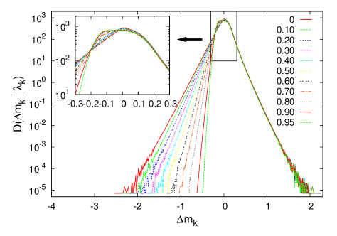
Total money remains constant in the steady state for any agent. An agent with a relatively higher $\lambda$ incurs losses which are considerably small in magnitude. This immediately suggests that agents with larger savings must be having more exchanges where losses, however small, occur. The magnified portion of the distribution shows that it is really so (shown in the inset of Fig. 2).

III.2 Walk in the wealth space: Definition

To investigate the dynamics at the microscopic level, one can conceive of a walk for the agents in the so called “wealth space”, in which each agent walks a step forward when she gains and one step backwards if she incurs a loss. The walks are correlated in the sense that when two agents interact, if one takes a step forward, the other has to move backward. On the other hand, two agents can interact irrespective of their positions in the wealth space unlike Brownian particles.

Once the system is in the steady state, we define $x(t+1)=x(t)+1$ if our tagged agent gains money, and $x(t+1)=x(t)-1$ if she loses. In other words, $x(t)$ performs a walk in one dimension. Without loss of generality we start from origin ($x(0)=0$), and we insist $t=0$ is well within the steady state. We investigate the properties of this walk by computing the mean displacement $\langle x(t)\rangle$, and the mean square displacement $\langle x^{2}(t)\rangle-\langle x(t)\rangle^{2}$.

Actually, one can also consider a walk for a tagged agent where the increments (i.e., step lengths) are the money gained or lost at each step, but the exponential distribution obtained for such step lengths (Fig. 2) indicates that it will be simple diffusion like Majumdar .

III.3 Results for the walk

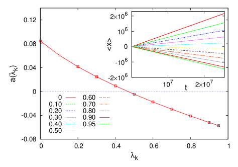
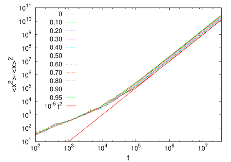
For the CC model, for any value of the fixed saving propensity $\lambda$, we obtain a conventional random walk in the sense $\langle x(t)\rangle$ is zero and $\langle x^{2}(t)\rangle-\langle x(t)\rangle^{2}\sim t$. However, for the CCM model, results are quite different. It is found that $\langle x(t)\rangle$ has a drift, $\langle x(t)\rangle\sim a(\lambda_{k})t$. $a(\lambda_{k})$ varies continuously with $\lambda_{k}$, taking positive to negative values as one goes from low to high values of savings $\lambda_{k}$ (see inset of Fig. 3) respectively. It is obvious that for some $\lambda_{k}^{*}$, there is no drift, $a(\lambda_{k}^{*})=0$. $\lambda_{k}^{*}$ is estimated to be about $0.469$ by interpolation method. On the other hand $\langle x^{2}\rangle-\langle x\rangle^{2}\sim t^{2}$ for all $\lambda_{k}$, which is a case of ballistic diffusion (Fig. 4).

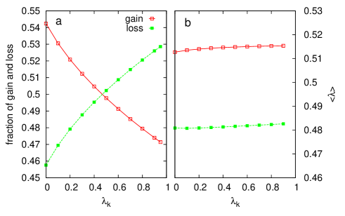
The negative or positive drifts of the walks indicate that the probabilities of gain and loss are not equal for any agent in general. Plotting the fraction of times the tagged agent gains/loses in Fig. 5(a), it is indeed found that an agent with a smaller $\lambda$ gains with more probability while the opposite happens for agents with larger $\lambda$. Indeed, the intersection of the two curves is the point $\lambda_{k}^{*}$ where the probabilities are equal and the corresponding walk should show $\langle x\rangle=0$. It is difficult, however, to detect numerically $\lambda_{k}^{*}$ exactly, which lies close to $0.47$, and check whether an agent with $\lambda_{k}^{*}$ behaves like a conventional random walker or shows ballistic diffusion. Simulations using values of $\lambda$ even very close to $0.47$ always show ballistic behavior.

Figure 3: Measures for the gain-loss walk: the inset shows $\langle x\rangle$ with time for different values of savings $\lambda_{k}$, showing the drifts. The slopes $a(\lambda_{k})$ are also shown. The estimate of $\lambda_{k}^{*}$ is approximately $0.469$. The data is shown for a system of $N=256$ agents.

Figure 4: Measures for the gain-loss walk: time variation of $\langle x^{2}\rangle-\langle x\rangle^{2}$ for different values of savings $\lambda_{k}$, and a guide to $t^{2}$. The data is shown for a system of $N=256$ agents.

In order to explain the above results, we investigate at a finer level the walk when the tagged agent with $\lambda_{k}$ interacts with another agent with saving $\lambda$. First, we calculate the average $\langle\lambda\rangle$ when the tagged agents loses or gains and find that for a gain, one has to interact with an agent with a higher $\lambda$ in general. This is shown in Fig. 5(b). In fact, the average value is very weakly dependent on $\lambda_{k}$ and significantly greater/less than 0.5 for a gain/loss. This is contrary to the expectation that gain/loss does not depend on the saving propensities of the interacting agents.

Figure 5: (a) Plot of probabilities of gain and loss for different values of savings propensity $\lambda_{k}$ of the tagged agent. The data is shown for a system of $N=256$ agents. (b) The plot of the average value $\langle\lambda\rangle$ when a gain/loss is being incurred shown against $\lambda_{k}$ of the tagged agent.

Having obtained evidence that gain/loss depends on the interacting agents’ saving propensities, we compute the probability of gain and loss, $P_{g}$ and $P_{l}$ respectively, as a function of $\lambda$ for the agent with saving $\lambda_{k}$. The data shows that indeed an agent gains with higher probability while interacting with an agent with $\lambda>\lambda_{k}$ and vice versa. In fact, the data for different $\lambda_{k}$ collapse when $P_{g}-P_{l}$ are plotted against a scaled variable $y=\frac{\lambda-\lambda_{k}}{1.5+\lambda_{k}+\lambda}$ as shown in Fig. 6 indicating a linear variation with $y$, i.e.,

$$P_{g}-P_{l}={\rm const}\frac{\lambda-\lambda_{k}}{1.5+\lambda_{k}+\lambda}.$$ (10)

We have checked that there is hardly any finite size effect on the collapse in the sense that the similarly scaled data for $N=100$ collapse exactly on those for $N=256$.

Figure 6: Data collapse for $\lambda_{k}=0.2,0.4,0.6$ and $0.8$ is shown for $P_{g}-P_{l}$ versus the scaled variable $y=\frac{\lambda-\lambda_{k}}{1.5+\lambda_{k}+\lambda}$ for $N=256$. The inset shows the unscaled data.

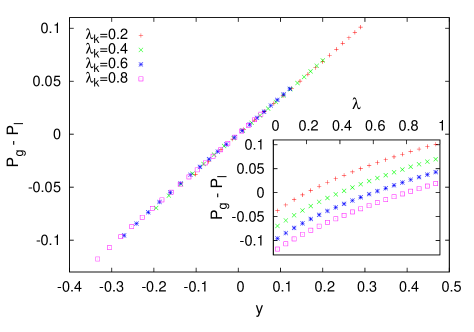
An agent with a high value of $\lambda$ will interact with a higher probability with agents whose saving propensities are lesser, causing a loss of money. Therefore in the wealth space it will have tendency to take more steps in the negative direction. This explains the negative drift for large $\lambda$.

It is possible to estimate the value of $\lambda_{k}^{*}$ using Eq. (10) utilizing the fact that the integrated value of $P_{g}-P_{l}$ over all $\lambda$ should be zero for $\lambda_{k}=\lambda_{k}^{*}$. This gives

$$1-(1.5+2\lambda_{k}^{*})\left[\log(2.5+\lambda_{k}^{*})-\log(1.5+\lambda_{k}^{*})\right]=0,$$ (11)

solving which we get $\lambda_{k}^{*}\simeq 0.4658$ which is consistent with the earlier observations.

It may be added here that in principle the probability of gain or of loss while two agents interact, can be calculated from the money distribution. In the CCM model, when two agents with money $m_{1}$ and $m_{2}$ and saving propensities $\lambda_{1}$ and $\lambda_{2}$ respectively, interact, the difference in money before and after transcation for, say, the second agent is given by $\left[(1-\lambda_{1})m_{1}-(1-\lambda_{2})m_{2}\right]/2$. Therefore for the second agent to lose, $m_{2}$ must be greater than $m^{\prime}=\frac{m_{1}(1-\lambda_{1})}{(1-\lambda_{2})}$ and the corresponding probability is given by

$$\int_{0}^{M}P(m_{1}|\lambda_{1})dm_{1}\int^{M}_{m^{\prime}}P(m_{2}|\lambda_{2})dm_{2}.$$ (12)

However, the exact form of the money distribution is not known Basu:2008 for the CCM case. For the CC model, $\lambda=\lambda_{1}=\lambda_{2}$ and letting $M\to\infty$, the above integral becomes

$$\int_{0}^{\infty}P(m_{1}|\lambda)dm_{1}\int^{\infty}_{m_{1}}P(m_{2}|\lambda)dm_{2}$$

$$=\int_{0}^{\infty}P(m_{1}|\lambda)[1-\tilde{P}(m_{1}|\lambda)]dm_{1},$$ (13)

where $\tilde{P}(m)=\int_{0}^{m}P(m)dm$ is the cumulative distribution of money. Since $P=\frac{\partial{\tilde{P}}}{\partial m}$, the R.H.S of Eqn. (13) is equal to 1/2 independent of the form of $P(m|\lambda)$. Thus in the CC case we find equal probability of gain or loss leading to a simple random walk. In the CCM, however, the results are expected to be dependent on $\lambda_{1},\lambda_{2}$ as (12) indicates.

IV Discussions

The analogy with a gas like many-body system has led to the formulation of the kinetic exchange models of markets. The random scattering-like dynamics of money (and wealth) in a closed trading market, in analogy with energy conserved exchange models, reveals interesting features. Self-organization is a key emerging feature of these simple models when saving factors are introduced. These models produce asset distributions resembling those observed in reality, and are quite well studied now Chatterjee:rev . These have prospective applications in other spheres of social science, as in application in policy making and taxation, and also physical sciences, possibly in designing desired energy spectrum for different types of chemical reactions.

In this paper, we have looked at the dynamics of agents at the scale of individuals. We study the distribution of money for a tagged agent given a particular value of saving propensity. We also analyze the distribution of money differences in successive exchanges. We conceived of a walk in an abstract space performed by the agents in different kinetic gas like models which reveals the characteristics of gains and losses made by the agents. Specifically, considering only whether an agent gains or loses, a walk can be defined in the wealth space, which is a random walk for the CC model while for the CCM model it is found to be ballistic in nature for generic values of $\lambda$.

On studying the dynamics at a microscopic level, we find that an agent gains with a higher probability when interacting with another agent with a larger $\lambda$. Thus one would expect, that for $\lambda=0.5$, there will be equal gains and losses which would give rise zero drift in the corresponding walk in the wealth space for the CCM model. The value of $\lambda_{k}^{*}$ for which we do get such a result is quite close to this estimate. An accurate estimate of $\lambda_{k}^{*}\simeq 0.4658$ is obtained by considering the scaling behavior of (probabilities of) gains and losses.

In the CCM model, our study leads to the discovery of the way gains and losses are dependent on the saving propensities of the agents, which cannot be arrived at using any existing results, either analytical or numerical. Using Eqn. (9), one can calculate the average money exchanged between two agents which turns out to be independent of their saving propensities. Hence the intriguing question that remains to be solved is why the probability of gain over loss depends on the savings of the interacting agents.