Abstract Fixpoint Computations
with Numerical Acceleration Methods

Abstract

Static analysis by abstract interpretation aims at automatically proving properties of computer programs. To do this, an over-approximation of program semantics, defined as the least fixpoint of a system of semantic equations, must be computed. To enforce the convergence of this computation, widening operator is used but it may lead to coarse results. We propose a new method to accelerate the computation of this fixpoint by using standard techniques of numerical analysis. Our goal is to automatically and dynamically adapt the widening operator in order to maintain precision.

Keywords: Abstract numerical domains, acceleration of convergence, widening operator.

1 Introduction

In the field of static analysis of embedded, numerical programs, abstract interpretation [8, 9] is widely used to compute over-approximations of the set of behaviors of a program. This set is usually defined as the least fixpoint of a monotone map on an abstract domain given by the (abstract) semantics of the program. Using Tarski’s theorem [18], this fixpoint is computed as the limit of the iterates of the abstract function starting from the least element. These iterates build a sequence of abstract elements that (order theoretically) converge towards the least fixpoint. This sequence converging often slowly (or even after infinitely many steps), the theory of abstract interpretation introduces the concept of widening [9].

A widening operator is a two-arguments function $\nabla$ which tries to predict the limit of the iterates based on the relative position of two consecutive iterates. For example, the standard widening operator on the interval abstract domain consists in comparing the limits of the intervals and setting the unstable ones to $\infty$ (or $-\infty$). A widening operator often makes large over-approximation because it must make the sequence of iterates converge in a finite time. Over-approximation may be reduced afterward using a narrowing operator but the precision of the final approximation still strongly depends on the precision of the $\nabla$. Various techniques have been proposed to improve it. Delayed widening makes use of $\nabla$ after $n$ iteration steps only (where $n$ is a user-defined integer), thus letting the first loop iterates execute before trying to predict the limit. Another approach is to use a widening with thresholds [2]: the upper bound of the interval (for example) is not directly set to $\infty$, but is successively increased using a set of thresholds that are candidates for the value of the fixpoint upper bound. In practice, these techniques are necessary to obtain precise fixpoint approximations for industrial sized embedded programs. However, they suffer from their lack of automatization: thresholds must be chosen a priori and are defined by the user (to the best of our knowledge, no methods exist to automatically find the best thresholds). The delay parameter $n$ is also to be defined a priori. This makes the use of a static analyzer difficult as these (non trivial) parameters are often hard to find.

In this article, we present some ongoing work which shows that it is possible to use sequence transformation techniques in order to automatically and efficiently derive approximation of the limit of Kleene iterates. This approximation may not be safe (i.e. may not contain the actual limit), but we show how to use it in the theory of abstract interpretation. Sequence transformation techniques (also known as convergence acceleration methods) are widely studied in the field of numerical analysis [5]. They transform a converging sequence $(x_{n})_{n\in{\mathbbm{N}}}$ of real numbers into a new sequence $(y_{n})_{n\in{\mathbbm{N}}}$ which converges faster to the same limit (see Section 3.2). In some cases (depending on the method), the acceleration is such that $(y_{n})_{n\in{\mathbbm{N}}}$ is ultimately constant. Some recent work [7] applied these techniques in the case of sequences of vectors of real numbers: vector sequence transformations introduce relations between elements of the vectors and perform better than scalar ones. Our main contribution is to show that we can use these methods in order to improve the fixpoint computation in static analysis: we define dynamic thresholds for widening that are very close to the actual fixpoint. This increased precision is obtained because the sequence transformations use all iterates and quantitative information (i.e. relative to the distance between elements) to predict the limit. They thus have access to more information than the widening operator and can make better prediction. In this work, we focus on the interval domain, but we believe that this work may be applied for any abstract domain, especially the ones with a pre-defined shape (octagons [16], templates [17], etc.).

This article is organized as follows. In Section 2, we explain on a simple example how acceleration methods may be used to speed-up the fixpoint computation. In Section 3, we recall the theoretical basis of this work and present our main theoretical contribution. Section 4 presents some early experiments on various floating-point programs that show the interest of our approach, while Sections 5 and 6 discuss related works and perspectives.

Notations. In the rest of this article, $(x_{n})$ will denote a sequence of real numbers (i.e. $(x_{n})\in{\mathbbm{R}}^{\mathbbm{N}}$), while $(\boldsymbol{x}_{n})$ denotes a sequence of vector of real numbers (i.e. $(\boldsymbol{x}_{n})\in\bigl{(}{\mathbbm{R}}^{p}\bigr{)}^{\mathbbm{N}}$ for some $p\in{\mathbbm{N}}$). The symbol $X_{n}$ will be used to design abstract iterates, i.e. $X_{n}\in A$ for some abstract lattice $A$.

2 An introductive example

In this section, we explain, using a simple example, how sequence acceleration techniques can be used in the context of static analysis. In short, our method works as follows: let $(X_{n})$ be a sequence of intervals computed by the Kleene iteration and that is chosen to be widened (see [4] for details on how to chose the widening points). We extract from $(X_{n})$ a vector sequence $(\boldsymbol{x}_{n})$: at stage $k$, $\boldsymbol{x}_{k}$ is a vector that contains the infimum and supremum of each variable of the program. As Kleene iterates converge towards the least fixpoint of the abstract transfer function, the sequence $(\boldsymbol{x}_{n})$ converges towards a limit $\boldsymbol{x}$ which is the vector containing the infimum and supremum of this fixpoint. We then compute an accelerated sequence $(\boldsymbol{y}_{n})$ that converges towards $\boldsymbol{x}$ faster than $(\boldsymbol{x}_{n})$. Once this sequence has reached its limit (or is sufficiently close to it), we use $\boldsymbol{x}$ as a threshold for a widening on $(\boldsymbol{x}_{n})$ and thus obtain, in a few steps, the least fixpoint. In the rest of this section, we detail these steps.

The program. We consider a linear program which iterates the function $F(X)=A\cdot X+B\cdot U$ where $A$, $B$ and $U$ are constant matrices and $X$ is the vector of variables (see Figure 1). Initially, we have $\texttt{x1}\in[1,2],\ \texttt{x2}\in[1,4],\ \texttt{x3}\in[1,20],\ \texttt{u1}\in[1,6],\ \texttt{u2}\in[1,4]$ and $\texttt{u3}\in[1,2]$. Using an existing analyzer working on the interval abstract domain, we showed that this program converges in 55 iterations (without widening) and obtained the invariant $[-5.1975,8.8733]$ for x1 at line $2$.

⬇

1 while (1) {

2 xn1 = -0.4375 * x1+ 0.0625 * x2 + 0.2652 * x3 + 0.1 * u1;

3 xn2 = 0.0625 * x1 + 0.4375 * x2 + 0.2652 * x3 + 0.1 * u2;

4 xn3 = -0.2652 * x1 + 0.2652 * x2 + 0.375 * x3 + 0.1 * u3;

5 x1 = xn1; x2 = xn2; x3 = xn3;

6 }

Figure 1: A simple linear program.

Extracting the sequences. From this program, we can define a vector sequence of size $6$,
$\boldsymbol{x}_{n}=\bigl{(}\underline{x^{1}_{n}},\overline{x^{1}_{n}},\underline{x^{2}_{n}},\overline{x^{2}_{n}},\underline{x^{3}_{n}},\overline{x^{3}_{n}}\bigr{)}$, which represent the evolution of the suprema and infima of the variables x1, x2 and x3 at line $2$. For example, the sequence $(\overline{x^{1}_{n}})$ is recursively defined by:

$$\overline{x^{1}_{n+1}}=\max\Bigl{(}\ \overline{x^{1}_{n}}\ ,\ -0.4375*\underline{x^{1}_{n}}+0.0625*\overline{x^{2}_{n}}+0.2652*\overline{x^{3}_{n}}+0.1*\overline{u_{1}}\ \Bigr{)}\;.$$ (1)

Note that we are not interested in the formal definition of these sequences (as given by Equation (1)), but only in their numerical values that are easily extracted from Kleene iterates. Each sequence $(\overline{x^{i}_{n}})$ (resp. $(\underline{x^{i}_{n}})$) is increasing (resp. decreasing) and the sequence $(\boldsymbol{x}_{n})$ converge towards a vector $\boldsymbol{x}$ containing the infimum and supremum of the fixpoint (see Figure 2, dotted lines).

Accelerating the sequences. We then used the vector $\varepsilon$-algorithm [7] to build a new sequence that converges faster towards $\boldsymbol{x}$. This method works as follows (a more formal definition will be given in Section 3.2): it computes a series of sequences $(\boldsymbol{\varepsilon}^{k}_{n})$ for $k=1,2,\dots$ such that each sequence $(\boldsymbol{\varepsilon}^{k}_{n})$ for $k$ even converges towards $\boldsymbol{s}$ and the diagonal $(\boldsymbol{d}_{n})=(\boldsymbol{\varepsilon}^{n}_{0})$ also converges towards $\boldsymbol{s}$. This diagonal sequence is the result of the $\varepsilon$-algorithm and is called the accelerated sequence. It converges faster than the original sequence: in only $8$ iterates, it reached the fixpoint and stayed constant (see Figure 2, bold lines).

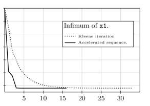
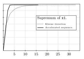
Figure 2: Sequences extracted from the program of Figure 1 and their accelerated version.

Using the accelerated sequence. When the accelerated sequence reaches the limit (or is sufficiently close to it), we modify the Kleene iteration and directly jump to the limit. Formally, if the limit is $(\underline{x_{1}},\overline{x_{1}},\underline{x_{2}},\overline{x_{2}},\underline{x_{3}},\overline{x_{3}})$ and if the current Kleene iterate is $X_{p}$, we construct the abstract element $X$ whose bounds are $\underline{x_{1}},\ \overline{x_{1}},\dots$ and set $X_{p+1}=X_{p}\cup X$ and re-start Kleene iteration from $X_{p+1}$. In this way, we remain sound ($X_{p}\subseteq X_{p+1}$) and we are very close to the fixpoint, as $X\subseteq X_{p+1}$. In this example, Kleene iteration stopped after $2$ steps and reached the same fixpoint as the one obtained without widening and acceleration. Figure 3 shows the original Kleene iteration and the modified one, for the infimum of variable x1. Let us recall that the Kleene iteration needed $55$ steps to converge, where the modified iteration stops after $18$ steps.

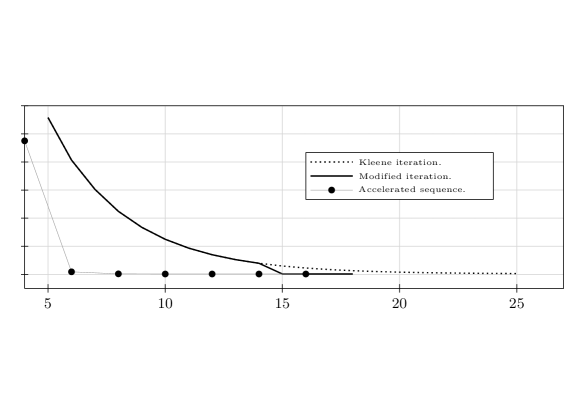
Figure 3: Infimum value of $x_{1}$. We only display the iterates $5$ to $25$. At the $15$th iteration, the accelerated value is used as a widening with thresholds, and the iteration stops after $18$ steps.

3 Theoretical frameworks

In this section, we briefly recall the basics of abstract interpretation, with an emphasis on the widening operator. Next we present in more details the theory of sequence transformations. Finally, we give our main contribution showing how sequence transformations are used in abstract interpretation theory.

3.1 Overview of the abstract interpretation theory

Abstract interpretation is a general method to compute over-approximations of program semantics where the two key ideas are:

• Safe abstractions of sets of states thanks to Galois connections. More precisely let $\langle C,\sqsubseteq_{C}\rangle$ be the lattice of concrete states and let $\langle A,\sqsubseteq_{A}\rangle$ be the lattice of abstract states. $A$ is a safe abstraction of $C$ if there exists a Galois connexion $\langle C,\sqsubseteq_{C}\rangle\mathrel{\hbox to0.0pt{\smash{\hskip 0.0pt\raisebox{-3.57222pt}{\hbox to24.47792pt{$\smash{-}\mkern-7.0mu\cleaders\hbox{$\mkern-2.0mu\smash{-}\mkern-2.0mu$}\hfill\mkern-7.0mu\mathord{\rightarrow}$}}}\hss}\hbox to0.0pt{\smash{\hskip 0.0pt\raisebox{-0.01561pt}{\hbox to24.47792pt{$\mathord{\leftarrow}\mkern-7.0mu\cleaders\hbox{$\mkern-2.0mu\smash{-}\mkern-2.0mu$}\hfill\mkern-7.0mu\smash{-}$}}}\hss}\hbox to0.0pt{\smash{\hskip 5.4269pt\raisebox{-4.73608pt}{\ $\scriptstyle\gamma$\ }}\hss}\hbox to0.0pt{\smash{\hskip 5.0pt\raisebox{6.13995pt}{\ $\scriptstyle\alpha$\ }}\hss}\rule[-6.09718pt]{0.0pt}{14.82045pt}\hskip 24.47792pt}\langle A,\sqsubseteq_{A}\rangle$, i.e. there exist monotone maps $\alpha$ and $\gamma$ such that $\forall c\in C,\forall a\in A,\alpha(c)\sqsubseteq_{A}a\Leftrightarrow c\sqsubseteq_{C}\gamma(a)$.

• An effective computation method of the abstract semantics with, in general, a widening operator. The semantics of a program is defined as the smallest solution of a recursive system of semantic equations $F$. Hence, the abstract program semantics is a set of states $X$ of a lattice $\langle A,\sqsubseteq_{A}\rangle$ such that $X=F(X)$ where $F$ is monotone. The solution $X$ is iteratively constructed by $X_{i+1}=X_{i}\sqcup F(X_{i})$, starting from $X_{0}=\bot$. The value $\bot$ denotes the smallest element of $A$ and the operation $\sqcup$ denotes the join operation of $A$. The sequence $(X_{n})$ defines an increasing chain of elements of $A$. This chain may be infinite, so to enforce the convergence of this sequence, we usually substitute the operator $\sqcup$ by a widening operator $\nabla$, see Definition 3.1, that is an over-approximation of $\sqcup$.

Definition 3.1 (Widening operator [8])

Let $\langle A,\sqsubseteq_{A}\rangle$ be a lattice. The map $\nabla:A\times A\rightarrow A$ is a widening operator iff i) $\forall v_{1},v_{2}\in A$, $v_{1}\sqcup v_{2}\sqsubseteq_{A}v_{1}\nabla v_{2}$. ii) For each increasing chain $v_{0}\sqsubseteq_{A}\cdots\sqsubseteq_{A}v_{n}\sqsubseteq_{A}\cdots$ of $A$, the increasing chain defined by $s_{0}=v_{0}$ and $s_{n}=s_{n-1}\nabla v_{n}$ is stationary: $\exists n_{0},\forall n_{1},n_{2},(n_{2}>n_{1}>n_{0})\Rightarrow s_{n_{1}}=s_{n_{2}}$.

The widening operator plays an important role in static analysis because, thanks to it, we are able to consider infinite state spaces. As a consequence, many abstract domains are associated with a widening operator. For example the classical widening of the interval domain is defined by:

$$[a,b]\nabla[c,d]=\left[\begin{cases}a&\text{if }a\leq c\\ -\infty&\text{otherwise}\end{cases},\quad\begin{cases}b&\text{if }b\geq d\\ +\infty&\text{otherwise}\end{cases}\right]\enspace.$$

Note that we only consider two consecutive elements to extrapolate the potential fixpoint. The main drawback with this widening is that it may generate too coarse results by going quickly to infinity. A solution of this is to add intermediate steps among a finite set $T$; that is the idea behind the widening with thresholds $\nabla_{T}$. For the interval domain, it is defined [3] by:

$$[a,b]\nabla_{T}[c,d]=\left[\begin{cases}a&\text{if }a\leq c\\ \max\{t\in T:t\leq c\}&\text{otherwise}\end{cases},\quad\begin{cases}b&\text{if }b\geq d\\ \min\{t\in T:t\geq d\}&\text{otherwise}\end{cases}\right]\enspace.$$

While widening with thresholds gives better results, we are facing with the problem to define a priori the set $T$. Finding relevant values for $T$ is a difficult task for which, to the best of our knowledge, no automatic solution exists.

3.2 Acceleration of convergence

We give an overview of the techniques of acceleration of convergence in numerical analysis [5]. The goal of convergence acceleration techniques, also named sequence transformations, is to increase the rate of convergence of a sequence. Formally, let $\bigl{(}D,d\bigr{)}$ be a metric space, i.e. a set $D$ with a distance $d:D\rightarrow{\mathbbm{R}}^{+}$ ($D$ will be ${\mathbbm{R}}$ or ${\mathbbm{R}}^{p}$ for some $p\in{\mathbbm{N}}$). The set of sequences over $D$ (denoted $D^{\mathbbm{N}}$) is the set of functions between ${\mathbbm{N}}$ and $D$. A sequence $(x_{n})\in D^{\mathbbm{N}}$ converges to $\ell$ iff we have $\lim_{n\rightarrow\infty}d(x_{n},\ell)=0$. A sequence transformation is a function $T:D^{\mathbbm{N}}\rightarrow D^{\mathbbm{N}}$ ($T$ designs a particular acceleration method) such that whenever $(x_{n})$ converges to $\ell$ then $(y_{n})=T(x_{n})$ also converges to $\ell$ and $\lim_{n\rightarrow\infty}\frac{d(y_{n},\ell)}{d(x_{n},\ell)}=0$. This means that $(y_{n})$ is asymptotically closer to $\ell$ than $(x_{n})$. An important notion for a sequence transformation $T$ is its kernel $K_{T}$ which is the set of sequences $(x_{n})$ for which $T(x_{n})$ is ultimately constant. We now present some acceleration methods that we used in our experimentation. For more details, we refer to [5].

The Aitken $\Delta^{2}$-method. It is probably the most famous sequence transformation. Given a sequence $(x_{n})\in{\mathbbm{R}}^{\mathbbm{N}}$, the accelerated sequence $(y_{n})$ is defined by: $\forall n\in{\mathbbm{N}},\ y_{n}=x_{n}-\frac{x_{n+1}-x_{n}}{x_{n+2}-2x_{n+1}+x_{n}}$. It should be noted that in order to compute $y_{n}$ for some $n\in{\mathbbm{N}}$, three values of $(x_{n})$ are required: $x_{n}$, $x_{n+1}$ and $x_{n+2}$. The kernel $K_{\Delta^{2}}$ of this method is the set of all sequences of the form $x_{n}=s+a.\lambda^{n}$ where $s$, $a$ and $\lambda$ are real constants such that $a\neq 0$ and $\lambda\neq 1$ (see [6]). The Aitken $\Delta^{2}$-method is an efficient method for accelerating sequences, but it highly suffers from numerical instability when $x_{n}$, $x_{n+1}$ and $x_{n+2}$ are close to each other.

The $\varepsilon$-algorithm. It is often cited as the best general purpose sequence transformation for slowly converging sequences [19]. From a converging sequence $(x_{n})\in{\mathbbm{R}}^{\mathbbm{N}}$ with limit $\ell$, the $\varepsilon$-algorithm builds the following sequences:

$$(\varepsilon^{-1}_{n}) :\forall n\in{\mathbbm{N}},\varepsilon^{-1}_{n}=0,$$ (2)

$$(\varepsilon^{0}_{n}) :\forall n\in{\mathbbm{N}},\varepsilon^{0}_{n}=x_{n},$$ (3)

$$(\varepsilon^{k}_{n}) :\forall k\geq 1,\ n\in{\mathbbm{N}},\ \varepsilon^{k+1}_{n}=\varepsilon^{k-1}_{n+1}+\bigl{(}\varepsilon^{k}_{n+1}-\varepsilon^{k}_{n}\bigr{)}^{-1}$$ (4)

The sequence $(\varepsilon^{k}_{n})$ is called the $k$-th column, and its construction can be graphically represented as on Figure 4. The even columns $(\varepsilon^{2k}_{n})$ (in gray on Figure 4) converge faster to $\ell$. The even diagonals $(\varepsilon^{2k}_{n})_{k\in{\mathbbm{N}}})$ also converge faster to $\ell$. In particular, the first diagonal (circled on Figure 4) converges very quickly to $\ell$, and it is the accelerated sequence. Let us remark that in order to compute the $n$-th element of that sequence, $2n$ elements of $(x_{n})$ are required.

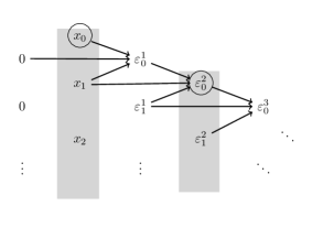
Arrows depict dependencies: the element at the beginning of the arrow is required to compute the element at the end. For example,

$$\varepsilon_{0}^{2} =\varepsilon_{1}^{0}+\frac{1}{\varepsilon_{1}^{1}-\varepsilon_{0}^{1}}$$

$$=x_{1}+\frac{1}{\varepsilon_{2}^{-1}+\frac{1}{\varepsilon_{2}^{0}-\varepsilon_{1}^{0}}-\varepsilon_{1}^{-1}+\frac{1}{\varepsilon_{1}^{0}-\varepsilon_{0}^{0}}}$$

$$=x_{1}+\frac{1}{\frac{1}{x_{2}-x_{1}}-\frac{1}{x_{1}-x_{0}}}$$

Figure 4: The $\varepsilon$-table

Acceleration of vector sequences. Many acceleration methods were designed to handle scalar sequences of real numbers. For almost each of these methods, extensions have been proposed to handle vector sequences (see [14] for a review of them). The simplest, yet one of the most powerful, of these methods is the vector $\varepsilon$-algorithm (VEA). Given a vector sequence $(\boldsymbol{x}_{n})$, the VEA computes a series of vector sequences $(\boldsymbol{\varepsilon}^{k}_{n})$ using Equations (2)-(4) where the arithmetic operations $+$ and $-$ are computed component-wise and the inverse of a vector $\boldsymbol{v}$ is computed as $\boldsymbol{v}^{-1}=\boldsymbol{v}/(\boldsymbol{v}\cdot\boldsymbol{v})$, with $/$ being the component-wise division and $\cdot$ the scalar product. The VEA differs from a component-wise application of the (scalar) $\varepsilon$-algorithm as it introduces relations between the components of the vector: the scalar product $\boldsymbol{v}\cdot\boldsymbol{v}$ computes a global information on the vector $\boldsymbol{v}$ which is propagated to all components. Our experiments show that this algorithm works better than a component-wise application of the $\varepsilon$-algorithm. The kernel $K_{\varepsilon}$ of the VEA contains all sequences of the form $\boldsymbol{x}_{n+1}=A\boldsymbol{x}_{n}+B$, where $A$ is a constant matrix and $B$ a constant vector [7].

3.3 Our contribution

In this section, we combine acceleration methods with the abstract fixpoint computation. Our goal is to be as non-intrusive as possible in the classical iterative scheme. In this way, our method can be implemented with minor adaptations in current static analyzers.

Methodology. As seen in Section 3.1, the Kleene iteration for finding the least fixpoint computes with abstract values from some abstract lattice $A$. In order to use acceleration techniques on the abstract iterates, we need to extract from the abstract elements $X_{n}\in A$ a vector of real numbers. Thus, we obtain a sequence of real vectors that we can accelerate, and we quickly reach its limit. We then construct an abstract element $X$ that corresponds to this limit and use it as a candidate for the least fixpoint. This process of transforming an abstract value into a real vector and back is formalized by the notion of extraction and combination functions that are given in Definition 3.2.

Definition 3.2 (Extraction and combination.)

Let $\langle A,\sqsubseteq_{A}\rangle$ be an abstract domain, and let $p\in{\mathbbm{N}}$. The functions $\Lambda_{A}:A\rightarrow{\mathbbm{R}}^{p}$ and $\Upsilon_{A}:{\mathbbm{R}}^{p}\rightarrow A$ are called extraction and combination function, respectively, iff for each sequence $X_{n}\in A^{\mathbbm{N}}$ that order theoretically converges, i.e. $\sqcup_{n\in{\mathbbm{N}}}X_{n}=X$ for some $X\in A$, then the sequence $\Lambda_{A}(X_{n})\in\bigl{(}{\mathbbm{R}}^{p}\bigr{)}^{\mathbbm{N}}$ converges for the usual metric on ${\mathbbm{R}}^{p}$, i.e. $\lim_{n\rightarrow\infty}\Lambda_{A}(X_{n})=S$, and $X\sqsubseteq_{A}\Upsilon_{A}(S)$.

Intuitively, these functions transpose the convergence of the sequence of iterates into the theory of real sequences, in such a way that the real sequence does not lose any information. Note that the order on ${\mathbbm{R}}^{p}$ induced by the usual metric is unrelated with the order $\sqsubseteq_{A}$ on $A$, so the notion of extraction and combination is different from the notion of Galois connection used to compare abstract domains. For the interval domain $I=\mathbbm{I}^{v}$, where $v$ is the number of variables of the program and $\mathbbm{I}$ is the set of floating-point intervals, the extraction and the combination functions are defined in Equation. (5).

For other domains, these functions must be designed specifically. For example, we believe that such functions can be easily defined for the octagon abstract domain [16]: the function $\Lambda$ associates with a difference bound matrix a vector containing all its coefficients. Special care should be taken in the case of infinite coefficients. More generally, we believe that for domains with a pre-defined shape, the functions $\Lambda$ and $\Upsilon$ can be easily defined. Note that if there is a Galois connection $(\alpha_{I},\gamma_{I})$ between a domain $A$ and the interval domain $I$, the extraction and combination functions can be defined as $\Lambda_{A}=\Lambda_{I}\circ\alpha_{I}$ and $\Upsilon_{A}=\gamma_{I}\circ\Upsilon_{I}$. We use this method in the last experiment in Section 4.2.

$$\Lambda_{I} :\left\{\begin{array}[]{rcl}I&\rightarrow&{\mathbbm{R}}^{2v}\\ (i_{1},\dots,i_{v})&\mapsto&\bigl{(}\overline{i_{1}},\underline{i_{1}},\dots,\overline{i_{V}},\underline{i_{V}}\bigr{)}\end{array}\right.$$ (5)

$$\Upsilon_{I} :\left\{\begin{array}[]{rcl}{\mathbbm{R}}^{2v}&\rightarrow&I\\ (x_{1},x_{2},\dots,x_{2v-1},x_{2v})&\mapsto&\bigl{(}[x_{1},x_{2}],\dots,[x_{2v-1},x_{2v}]\bigr{)}\end{array}\right.$$

Accelerated abstract fixpoint computation. We describe the insertion of acceleration methods in the Kleene iteration process in Algorithm 1. We compute in parallel the sequence $(X_{n})$ coming from the Kleene’s iteration and the accelerated sequence $(\boldsymbol{y}_{n})$ computed from an accelerated method. Once the sequence $(\boldsymbol{y}_{n})$ seems to converge, that is the distance between two consecutive elements of $(\boldsymbol{y}_{n})$ is smaller than a given value $\delta$, we combine the two sequences. That is we compute the upper bound of the two elements of the current iteration. Note that the monotonicity of the computed sequence $(X_{n})$ is still guaranteed.

Algorithm 1 Accelerated abstract fixpoint computation

1:  repeat

2:     $X_{i}:=X_{i-1}\ \sqcup\ F(X_{i-1})$

3:     $\boldsymbol{y}_{i}:=\text{Accelerate}\left(\Lambda_{A}(X_{0}),\dots,\Lambda_{A}(X_{i})\right)$

4:     if $||\boldsymbol{y}_{i}-\boldsymbol{y}_{i-1}||\ \leq\ \delta$ then

5:        $X_{i}:=X_{i}\ \sqcup\ \Upsilon_{A}(\boldsymbol{y}_{i})$

6:     end if

7:  until $X_{i}\sqsubseteq X_{i-1}$

The use of acceleration methods may be seen as an automatic delayed application of the widening with thresholds. Let us remark that we are not guaranteed to terminate in finitely many iterations: we know that asymptotically, the sequence $\boldsymbol{y}_{i}$ from Algorithm 1 gets closer and closer to the fixpoint, but we are not guaranteed that it reaches it. To guarantee termination of the fixpoint computation, we have to use more “radical” widening thresholds, for example after $n$ applications of the accelerated method. So this method cannot be a substitute to widening, but it improves it by reducing the number of parameters (delay and thresholds) that a user must define.

4 Experimentation

To illustrate our acceleration methods, we used a simple static analyzer working on the interval abstract domain that handles C programs without pointers and associated it with our OCaml library of acceleration methods that transform an input sequence (given as a sequence of values) into its accelerated version. The obtained results are presented in the following sections.

4.1 Butterworth order $1$

To test the acceleration method, we use a first-order Butterworth filter (see Figure 5, left). This filter is designed to have a frequency response which is as flat as mathematically possible in the band-pass and is often used in embedded systems to treat the input signals for a better stability of the program.

⬇

x1 = 0; y = 0; xn1 = 1;

for (i=0;i<200;i++) {

/*!npk u between 1 and 2 */

xn1 = 0.90480*x1 + 0.95240*u;

y = 0.09524*x1 + 0.04762*u;

x1 = xn1;

}

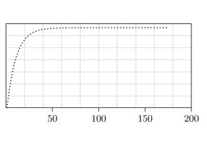
Figure 5: The Butterworth program (left) and the sequence of supremum of variable x1 (right).

The static analysis of this program using the interval abstract domain defines $10$ sequences, two for each variable (x1, xn1, y, u, i). These sequences converge toward the smallest fixpoint after a lot of iterations, our acceleration methods allow to obtain the same fixpoint faster. In this example, we accelerate just the upper bound sequences because the lower ones are constant for all the variables. We next present the result obtained with different methods on the variable x1 only, results obtained with other variables are very alike.

The Aitken $\Delta^{2}$-method. In Figure 5, right, with Kleene iteration and without widening, this program converges in $156$ iterations, and we get the invariant $[0,20.0084]$ for x1. With the Aitken $\Delta^{2}$-method, we obtain only in $3$ iterations a value very close to $20.0084$, but problems of numerical instabilities prevent the stabilization of the program. However the values of the accelerated sequence stay in the interval $[20.0082,20.0086]$ between the third and the last iteration (see Figure 6, left), which is a good estimate of the convergent point.

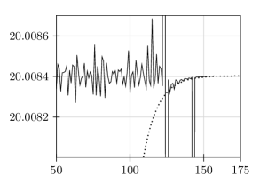
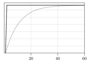
Figure 6: Accelerated sequences (in bold) compared with the original Kleene sequence (dotted). Left is the sequence obtained with Aitken (zooming on the numerical problems), right with the $\varepsilon$-algorithm (zooming on the first iterates).

The $\varepsilon$-algorithm. In Figure 6, right, we notice a important amelioration in the computation of the fixpoint, thanks to the $\varepsilon$-algorithm. With this method, the fixpoint of the variable x_1 is approximated with a precision of $10^{-6}$ after exactly $8$ iterations, while Kleene iteration needed $156$ steps. Remark that to obtain $8$ elements of the accelerated sequence we need $16$ elements from the initial one. We obtain the same results with the vector $\varepsilon$-algorithm.

4.2 Butterworth order $2$

An order 2 Butterworth filter is given by the following recurrence equation, where $\boldsymbol{x_{n}}$ is a two-dimensional vector, $\boldsymbol{x}_{n}=(x_{1},x_{2})^{T}$:

$$\boldsymbol{x}_{n+1}=\begin{pmatrix}0.9858&-0.009929\\ 0.00929&1\end{pmatrix}\cdot\boldsymbol{x}_{n}+u\cdot\begin{pmatrix}0.9929\\ 0.004965\end{pmatrix},\quad y_{n+1}=\begin{pmatrix}4.965e^{-5}\\ 0.01\end{pmatrix}\cdot\boldsymbol{x_{n}}+2.482e^{-5}\cdot u$$

Variable	Kleene	Vector $\varepsilon$-algorithm (Before + After)
		$\delta=10^{-3}$	$\delta=10^{-4}$	$\delta=10^{-5}$
$x_{1}$	$70$	$7~{}(6+1)$	$9~{}(8+1)$	$22~{}(16+6)$
$x_{2}$	$83$	$26~{}(6+20)$	$23~{}(8+15)$	$17~{}(16+1)$
$y$	$83$	$26~{}(6+20)$	$23~{}(8+15)$	$19~{}(16+3)$

Before: number of iterations to reach the condition on $\delta$. After: the remaining number of Kleene iterations to reach the invariant using the accelerated result.

Figure 7: Numbers of iterations needed to reach an invariant.

On this program, the results obtained using the interval abstract domain are not stable. To address this problem we have used Fluctuat [13], a static analyzer using a specific abstract domain based on affine arithmetic, a more accurate extension of interval arithmetic. It returns the upper and lower bounds of each variables. We applied the vector $\varepsilon$-algorithm on this example with 3 different values of $\delta$ (see Algorithm 1): this gives Figure 7. For example, for the variable $x_{1}$ and $\delta=10^{-3}$, the over-approximation of the fixpoint is reached after $26$ iterations ($6$ iterations before re-injection and $20$ iterations after). Note that we obtain the same fixpoint as with Kleene iteration. We notice that the performance of the Algorithm 1 does not strongly depend of $\delta$. Until now, we use the acceleration just once (unlike in Algorithm 1), a full implementation of it will probably reduce the number of iterations even more.

5 Related work

Most of the work in abstract interpretation based static analysis concerned the definition of new abstract domains (or improvements of existing ones), and the abstract fixpoint computation remained less studied. Initial work from Cousot and Cousot [9] discussed various methods to define widening operators. Bourdoncle [4] presented different iteration strategies that help reducing the over-approximation introduced by widening. These methods are complementary to our technique: as explained in Section 3.3, acceleration should be done at the same control point as the one chosen for widening, and does not replace standard widening as the termination of the fixpoint computation is not guaranteed. However, acceleration methods greatly improve widening by dynamically and automatically finding good thresholds.

Gopan and Reps in their guided static analysis framework [11, 12] also used the idea of computing in parallel the main iterates and a guide that shows where the iterates are going. In their work, the precision of the fixpoint computation is increased by computing a pilot value that explores the state space using a restricted version of the iteration function. Once this pilot has stabilized, it is used to accelerate the main iterates; in a sense, this pilot value is very similar to the value $\boldsymbol{y}_{i}$ of Algorithm 1, but we do not modify the iteration function as done in [12].

Maybe the work that is the closest to ours is the use of acceleration techniques in model checking [1], that have recently been applied to abstract interpretation [10, 15]. In this framework, the term acceleration is used to describe techniques that try to predict the effect of a loop on an abstract state: the whole loop is then replaced with just one transition that safely and precisely approximates it. These techniques perform very well for sufficiently simple loops working on integer variables, and gives exact results for such cases. Again, this method is complementary to our usage of acceleration: it statically modifies the iteration function by replacing simple loops with just one transition, while our method dynamically predicts the limit of the iterates. We believe that our method is more general, as it can be applied to many kinds of loops and is not restricted to a specific abstract domain (changing the abstract domain only requires changing the $\Lambda_{A}$ and $\Upsilon_{A}$ functions).

6 Conclusion

We presented in this article, a technique to accelerate abstract fixpoint computations using the numerical acceleration methods. This technique consists in building numerical sequences by extracting, at every iteration, supremum and infimum from every variable of the program. We apply to the obtained sequences the various convergence acceleration methods, that allows us to get closer significantly or to reach the fixpoint more quickly than the Kleene iteration. To make sure that the fixpoint returned by the accelerated method is indeed the fixpoint of the abstract semantics, we re-inject it in the static analyzer. This guarantees us the fast stop of the analyzer with a good over-approximation of the fixpoint. The experiments made on a certain number of examples (linear programs) show a good acceleration of the fixpoint computation especially when we use the $\varepsilon$-algorithm, where the number of iterations is divided by four. Let us note that we have assumed in this article that the sequences of iterates and the corresponding vector sequences converge towards a finite limit. In case of diverging sequences, traditional widening can be used as sequence transformation will not perform as well as for converging ones.

For now, we made the experimentation using two separate programs: one that computes the Kleene iterates, and one that accelerates the sequences. The Algorithm 1 is thus still not fully implemented, its automatization is the object of our current work. The use of the interval abstract domain allows to cover just a small set of programs, our future work will also consist in extending this technique to relational domains such as octagons and polyhedra.

References

- [1] Sébastien Bardin, Alain Finkel, Jérôme Leroux, and Laure Petrucci. FAST: acceleration from theory to practice. Journal on Software Tools for Technology Transfer, 10(5):401–424, 2008.
- [2] B. Blanchet, P. Cousot, R. Cousot, J. Feret, L. Mauborgne, A. Miné, D. Monniaux, and X. Rival. Design and implementation of a special-purpose static program analyzer for safety-critical real-time embedded software. In The Essence of Computation: Complexity, Analysis, Transformation, volume 2566 of LNCS, pages 85–108. Springer, 2002.
- [3] Bruno Blanchet, Patrick Cousot, Radhia Cousot, Jérôme Feret, Laurent Mauborgne, Antoine Miné, David Monniaux, and Xavier Rival. A Static Analyzer for Large Safety-Critical Software. In Programming Language Design and Implementation, pages 196–207. ACM Press, 2003.
- [4] Francois Bourdoncle. Efficient chaotic iteration strategies with widenings. In Proceedings of the International Conference on Formal Methods in Programming and their Applications, pages 128–141. Springer-Verlag, 1993.
- [5] Claude Brezinski and M. Redivo Zaglia. Extrapolation Methods-Theory and Practice. North-Holland, 1991.
- [6] Claude Brezinski and Michela Redivo Zaglia. Generalizations of aitken’s process for accelerating the convergence of sequences. Computational and Applied Mathematics, 2007.
- [7] Claude Brezinski and Michela Redivo Zaglia. A review of vector convergence acceleration methods, with applications to linear algebra problems. International Journal of Quantum Chemistry, 109(8):1631–1639, 2008.
- [8] P. Cousot and R. Cousot. Abstract interpretation: a unified lattice model for static analysis of programs by construction or approximation of fixpoints. In Principles of Programming Languages, pages 238–252. ACM Press, 1977.
- [9] P. Cousot and R. Cousot. Comparing the Galois connection and widening/narrowing approaches to abstract interpretation. In Programming Language Implementation and Logic Programming, volume 631 of LNCS, pages 269–295. Springer, 1992.
- [10] Laure Gonnord and Nicolas Halbwachs. Combining widening and acceleration in linear relation analysis. In Static Analysis Symposium, volume 4134 of LNCS, pages 144–160. Springer, 2006.
- [11] Denis Gopan and Thomas W. Reps. Lookahead Widening. In Computer Aided Verification, volume 4144 of LNCS, pages 452–466. Springer, 2006.
- [12] Denis Gopan and Thomas W. Reps. Guided static analysis. In Static Analysis Symposium, volume 4634 of LNCS, pages 349–365. Springer, 2007.
- [13] Eric Goubault, Matthieu Martel, and Sylvie Putot. Asserting the precision of floating-point computations: a simple abstract interpreter. In European Symposium on Programming, volume 2305 of LNCS, pages 209–212. Springer, 2002.
- [14] P. R. Graves-Morris. Extrapolation methods for vector sequences. Numerische Mathematik, 61(4):475–487, 1992.
- [15] Jérôme Leroux and Grégoire Sutre. Accelerated data-flow analysis. In Static Analysis Symposium, volume 4634 of LNCS, pages 184–199. Springer, 2007.
- [16] A. Miné. Weakly Relational Numerical Abstract Domains. PhD thesis, École Polytechnique, Palaiseau, France, 2004.
- [17] Sriram Sankaranarayanan, Henny B. Sipma, and Zohar Manna. Scalable analysis of linear systems using mathematical programming. In Verification, Model Checking, and Abstract Interpretation, volume 3385 of LNCS, pages 25–41. Springer, 2005.
- [18] A. Tarski. A lattice-theoretical fixpoint theorem and its applications. Pacific Journal of Mathematics, 5:285–309, 1955.
- [19] P. Wynn. The epsilon algorithm and operational formulas of numerical analysis. Mathematics of Computation, 15(74):151–158, 1961.