Charge tunneling in fractional edge channels

Abstract

We explain recent experimental observations on effective charge of edge states tunneling through a quantum point contact in the weak backscattering regime. We focus on the behavior of the excess noise and on the effective tunneling charge as a function of temperature and voltage. By introducing a minimal hierarchical model different filling factors, $\nu=p/(2p+1)$, in the Jain sequence are treated on equal footing, in presence also of non-universal interactions. The agreement found with the experiments for $\nu=2/3$ and $\nu=2/5$ reinforces the description of tunneling of bunching of quasiparticles at low energies and quantitatively defines the condition under which one expects to measure the fundamental quasiparticle charge. We propose high-order current cumulant measurement to cross-check the validity of the above scenario and to better clarify the peculiar temperature behavior of the effective charges measured in the experiments.

I Introduction

Fractional quantum Hall effect represents one of the most important examples of strongly correlated electron system DasSarma97 . In the bulk, quasiparticle (qp) excitations are predicted to have fractional charge Laughlin83 which, e.g., for filling factor in the Jain series, $\nu=p/(2p+1)$ ($p\in\mathbb{Z}$), is $e^{*}=e(\nu/|p|)$. At the edge Wen90 ; Wen91 ; Wen95 the identification of these charge excitations seems more complicated. Indeed, while in the past measurements of current noise through quantum point contacts (QPC), in the weak backscattering regime, confirmed the tunneling of single-qpdePicciotto97 ; Seminadayar97 , recently, new measurements have demonstrated the possibility of tunneling charges multiple of the fundamental charge. The condition to observe a bunching of qp depends on the external parameters such as temperature and voltage. MeasurementsChung03 carried out for the Jain series ($p=2,3$), at extremely low temperatures, show an effective charge equal to $e_{\rm eff}=\nu e$, which, only by increasing the temperature, decreases to the fundamental value $e_{\rm eff}=e^{*}$. Last year, experimental results for filling factor $\nu=2/3$ $(p=-2)$ appeared Ofek09 , showing a similar crossover. This common trend was very recently verified also for filling factor outside the Jain series belonging to fractional values in the second Landau level dolev10 .

In addition to the bunching phenomena peculiar behavior also appears in the backscattering current at high transparencies. For example for $\nu=1/3$, the current was found to increase with temperature Chung03 ; Roddaro04 instead of decrease as theoretically predicted Fendley95 . This support the indication of a non-universal renormalization of the tunneling exponents induced by the presence of edge interaction with external environment Rosenow02 , electron-electron interaction Papa04 ; Mandal02 and edge reconstruction Yang03 ; Aleiner94 .

In order to describe the Jain sequence different models were proposed with the common requirement of the presence of neutral modes in order to fulfill the statistical properties. One could have $|p|-1$ neutral fields propagating at finite velocity along the edge Wen92 ; Kane94 ; Kane95 , or only two or one - for infinite edges - additional modes with zero Lopez99 ; Lopez01 or finite velocity Ferraro08 . A peculiar characteristic, associated to the neutral modes is their direction of propagation with respect to the charged mode. Depending on the sign of $p$ and the theoretical model, there is the possibility to have co-propagating or counter-propagating neutral modes.

The tendency of bunching of qp at low temperature and weak backscattering was underlined in theory for the hierarchy of the Jain sequence Kane94 ; Kane95 ; Ferraro08 . In Ref. Ferraro08, we pointed out the role of propagating neutral modes in order to fully describe the experimental data Chung03 for $p>1$. By comparing with experiments for $\nu=2/5$ it was indeed possible to estimate the energy bandwidth of neutral modes.

Despite the presence of different proposals on the direct detection of neutral modes Levin07 ; Feldman08 ; Ferraro08 ; Overbosch09 ; Ferraro09b ; Cappelli09 ; Cappelli10 ; Yang09 , experiments addressed this issue only recently Granger09 ; Aveek10 .

In this paper we present a minimal hierarchical model able to include all the essential features of the above different proposal using few free parameters. This allows to explain, in an unified background, the experimental results of tunneling of effective charges in a standard quantum point contact geometry at extremely high transmission Chung03 ; Ofek09 . The dependence of the excess noise on the external parameters such as the voltage and the temperature is quantitatively analyzed. The flexibility of the proposed model resides on the possibility to link the results obtained in the presence of counter-propagating or co-propagating neutral modes. We demonstrate that both cases reproduce the experimental results using a proper choice of the fitting parameters.

We also propose the skewness, namely the normalized third backscattering current cumulant, as a measurable quantity Reulet03 ; Lindell04 ; Bomze05 ; Huard07 ; Timofeev07 ; Gershon08 able to give independent information on the nature of the carriers. This quantity is a good estimator of the crossover in the tunneling between the bunching of qp and the fundamental charge. We show that this quantity can be directly compared with the effective charge measured in the experiments by fitting the excess noise, as a function of the bias voltage, at fixed values of temperature.

II Model

We consider infinite edge states of an Hall bar with filling factor in the Jain series $\nu=p/(2p+1)$ ($p\in\mathbb{Z}$). The model adopted is a minimal one with two decoupled bosonic fields, one charged $\varphi^{\rm{c}}$ and one neutral $\varphi^{\rm{n}}$. The Euclidean free action is ($\hbar=1$, $k_{\rm B}=1$)

$$\mathcal{S}^{0} =\frac{1}{4\pi\nu}\int^{\beta}_{0}\!\!\!d\tau\!\!\int^{+\infty}_{-\infty}\!\!\!\!\!\!dx\partial_{x}\varphi^{\rm{c}}(x,\tau)\left(i\partial_{\tau}+v_{\rm{c}}\partial_{x}\right)\varphi^{\rm{c}}(x,\tau)+$$ (1)

$$+\frac{1}{4\pi}\int^{\beta}_{0}\!\!\!d\tau\!\!\!\int^{+\infty}_{-\infty}\!\!\!\!\!\!\!dx\partial_{x}\varphi^{\rm{n}}(x,\tau)\left(i\xi\partial_{\tau}+v_{\rm{n}}\partial_{x}\right)\varphi^{\rm{n}}(x,\tau)\,,$$

with $\beta=T^{-1}$ the inverse temperature and $v_{\rm{c}}$, $v_{\rm{n}}$ the propagation velocities of charge and neutral modes respectively. The former is affected by Coulomb interactions Levkinskyi08 ; Levkinskyi09 such that $v_{\rm{c}}\gg v_{\rm{n}}$ Ferraro08 . We consider neutral modes co-propagating $(\xi=+1)$ or counter-propagating $(\xi=-1)$ with respect to the charged one. This choice allows a unified description of different hierarchical models. For $\xi={\rm{sgn}}(p)$ one recovers the restricted model of Lee and Wen Lee98 (LW), where the $|p|-1$ neutral modes are described in terms of a single one. While for $\xi=-{\rm{sgn}}(p)$ one obtains the generalized Fradkin-Lopez model Lopez99 ; Chamon07 ; Ferraro08 ; Ferraro09b (GFL) with a single neutral mode propagating at finite velocity instead of a topological one Lopez99 .

The commutators of the bosonic fields are $[\varphi^{\rm{c/n}}(x),\varphi^{\rm{c/n}}(y)]=i\pi\nu_{\rm{c/n}}\mathrm{sgn}(x-y)$ with $\nu_{\rm{c}}=\nu$ and $\nu_{\rm{n}}=\xi$. The electron number density depends on the charged field only, via the relation $\rho(x)=\partial_{x}\varphi^{\rm{c}}(x)/2\pi$.

Edge excitations. In the hierarchical theories admissible edge excitations have a well defined charge and statistics Wen92 ; Lopez99 . There are single-qp excitations with charge $e^{*}$ with $e^{*}=(\nu/|p|)e$ and multiple qp-excitations with charge $me^{*}$ ($m\in\mathbb{N}$)Note1 . Their statistics is fractional with statistical angle Su86

$$\theta_{m}=m^{2}\left(\frac{\nu}{p^{2}}-\frac{1}{p}-1\right)\pi\,\,\,\,\,\,\,(\rm{mod}\,\,2\pi).$$ (2)

In addition, the phase acquired by any excitation in a loop around an electron must be an integer multiple of $2\pi$ Froehlich97 ; Ino98 ; Ferraro09b . Using the bosonization technique and imposing the above constraints, one can write the $m$-multiple excitation operator Ferraro09b

$$\Psi^{(m,q)}(x)=\frac{\mathcal{F}^{(m,q)}}{\sqrt{2\pi a}}e^{i\left\{\left(s+\frac{d}{|p|}\right)\varphi^{\rm{c}}(x)+\sqrt{p^{2}-\xi p}\left(q+\frac{d}{|p|}\right)\varphi^{\rm{n}}(x)\right\}}$$ (3)

with $a$ cut-off length, $s\in\mathbb{N}$ and $0\leq d\leq|p|-1$ such that $m=s|p|+d$. The integer $q$ is an additional quantum number associated to the freedom of add $2\pi$ to the statistical angle Ferraro09b . The operator $\mathcal{F}^{(m,q)}$ changes the number of $m$-agglomerates on the edge and ensures the right statistical properties between different $q$-values and different edgesFerraro09b . It can be neglected in the sequential tunneling regime Ferraro09b ; Guyon02 ; Martin05 . The most general expression for an excitation with charge $me^{*}$ will be then given by a superposition of the above operator with different $q$ values Ferraro09b ; Wen95 .

Relevant excitations. The scaling dimension associated to an $(m,q)$-excitation is extracted from the long time limit of the two-point imaginary time Green’s function $\mathcal{G}^{(m,q)}(\tau)=\left\langle T_{\tau}\Psi^{(m,q)}(0,\tau){\Psi^{(m,q)}}^{\dagger}(0,0)\right\rangle$ at zero temperature Kane92 . For $|\tau|\gg\omega_{\rm{n}}^{-1},\omega_{\rm{c}}^{-1}$ it is $\mathcal{G}^{(m,q)}(\tau)\propto|\tau|^{-2\Delta_{m}(q)}$ with

$$\Delta_{m}(q)=\frac{g_{\rm{c}}\nu}{2}\!\left(\frac{m}{|p|}\right)^{2}\!\!\!+\!\frac{g_{\rm{n}}}{2}(p^{2}-\xi p)\!\left(q+\frac{d}{|p|}\right)^{2}.$$ (4)

Here, $\omega_{\rm{c,n}}=v_{\rm{c,n}}/a$ are the energy bandwidth and satisfy $\omega_{\rm{n}}\ll\omega_{\rm{c}}$. The first term in (4) is due to the charged mode, while the second is related to the neutral one. The parameters $g_{\rm c}$ and $g_{\rm n}$ are introduced to take into account possible interaction effects due to the external environment Rosenow02 ; Papa04 ; Mandal02 ; Yang03 . It is worth to note that the two models considered, with $\xi=\pm{\rm sgn}(p)$, differ in the neutral mode contribution only. However, introducing neutral renormalization parameters $g^{\rm{LW}}_{\rm{n}}$ and $g^{\rm{GFL}}_{\rm{n}}$ for the LW and the GFL model respectively, one can map the two cases via the substitution

$$g^{\rm{LW}}_{\rm{n}}=g^{\rm{GFL}}_{\rm n}\ \frac{p^{2}+|p|}{p^{2}-|p|}\ .$$ (5)

Operators with the minimal scaling dimension are the most relevant and dominate the transport properties at low energies $E\ll\omega_{\rm n},\omega_{\rm c}$ Kane92 ; Ferraro08 ; Ferraro09b . In the unrenormalized case $(g_{\rm c}=g_{\rm n}=1)$ the two most dominant excitations have always $q=0$. They correspond to the agglomerate with $m=|p|$ ($d=0$, $s=1$) and to the single-qp with $m=1$ ($d=1$, $s=0$). The corresponding scaling are

$$\Delta^{\rm min}_{|p|}=\frac{\nu}{2}\,,\qquad\Delta^{\rm min}_{1}=\frac{1}{2}\left[\frac{\nu}{p^{2}}\!\!+(1-\frac{\xi}{p})\right].$$ (6)

Note that among these two, the $|p|$-agglomerate is always the most relevant since $\Delta^{\rm min}_{|p|}<\Delta^{\rm min}_{1}$ with the only exception for $\nu=2/3$ in the LW model ($\xi=-1$), where both have equal scaling Wen92 ; Kane95 . At higher energies $\omega_{\rm n}\ll E\ll\omega_{\rm c}$ the neutral mode saturates and does not contribute to the scaling $\Delta_{m}$, which consequently depends on the charged mode only with a value $\Delta^{\rm eff}_{m}={\nu m^{2}}/{2p^{2}}$. Here, the single-qp ($m=1$) always dominate. This implies the possibility of a crossover regime from low energies (relevance of $|p|$-agglomerates) to higher energies (relevance of single-qp). In the presence of interactions, Eq.(4) shows the relevance of the $|p|$-agglomerate at low energies if $g_{\rm{n}}/g_{\rm{c}}>\nu(1+\xi/p)$, otherwise the single-qp will always dominate.

III Transport properties

Tunneling of a bunched $m$-excitations through the QPC located at $x=0$ is described by $H^{(m)}_{\rm{T}}=\textbf{t}_{m}{\Psi^{(m)}_{\rm{R}}}^{\dagger}(0)\Psi^{(m)}_{\rm{L}}(0)+{\rm h.c.}$ with amplitude $\textbf{t}_{m}$. The indices $\rm R$ and $\rm L$ represent the right and left edge of the Hall bar. We will consider only the relevant excitations with $m=1$ (single-qp) or $m=|p|$ ($|p|$-agglomerate). In the incoherent sequential regime and at lowest order in $H^{(m)}_{\rm{T}}$ higher current cumulants $\langle I^{(m)}_{\rm{B}}\rangle_{k}$ ($k$-th order cumulant) are expressed in terms of the backscattering current $I^{(m)}_{\rm{B}}$

$$\langle I^{(m)}_{\rm{B}}\rangle_{k}=\left\{\begin{array}[]{l}(me^{*})^{k-1}\coth\left(E_{m}/2T\right)I^{(m)}_{\rm{B}}\\ (me^{*})^{k-1}I^{(m)}_{\rm{B}}\end{array}\right.\begin{array}[]{l}k\,\,\,{\rm{even}}\\ k\,\,\,{\rm{odd}}\end{array}$$ (7)

since the statistics is bidirectional PoissonianLevitov04 . The current is proportional to the tunneling rate $\Gamma^{(m)}(E)$ as $I^{(m)}_{\rm{B}}=me^{*}(1-e^{-E_{m}/T})\Gamma^{(m)}(E_{m})$ with

$$\Gamma^{(m)}(E_{m})=\gamma_{m}^{2}\!\int^{+\infty}_{-\infty}\!\!\!\!\!\!dt^{\prime}e^{-iE_{m}t^{\prime}}e^{2\alpha^{2}_{m}\mathcal{D}^{>}_{\rm{c}}(t^{\prime})}e^{2\beta^{2}_{m}\mathcal{D}^{>}_{\rm{n}}(t^{\prime})}\,.$$ (8)

Here, $E_{m}=me^{*}V$, with $V$ the QPC bias voltage and $\gamma_{m}^{2}=|\textbf{t}_{m}|^{2}/(4\pi^{2}a^{2})$. The charge coefficient is $\alpha_{m}=m/|p|$ while the neutral one is given by the minimal value with $q=0$ in Eq.(3). For the single-qp it is $\beta_{1}^{2}=(1-\xi/p)$, while for the $|p|$-agglomerate it is $\beta_{|p|}=0$. The correlation functions Braggio01 ; Ferraro08 of charged and neutral modes are

$$\mathcal{D}^{>}_{r}(t)=g_{r}\nu_{r}\ln{\left[\frac{|\mathbf{\Gamma}\left(1+T/\omega_{r}-iTt\right)|^{2}}{\mathbb{\Gamma}^{2}\left(1+T/\omega_{r}\right)\left(1-i\omega_{r}t\right)}\right]},$$ (9)

with $r=\rm{c},\rm{n}$ and $\mathbb{\Gamma}(x)$ the Euler Gamma function. The rate is obtained by numerically evaluating (8) apart at zero temperature where analytical results are available Ferraro08 .

At lowest order, tunneling processes of different excitations are independent. The contributions of different excitations are then simply summed. In our case, the total $k$-th order cumulant will be given by the sum of the most relevant processes $\langle I_{\rm{B}}\rangle_{k}=\langle I^{(1)}_{\rm{B}}\rangle_{k}+\langle I^{(p)}_{\rm{B}}\rangle_{k}$. The trasmission of the QPC is then expressed in terms of the total backscattering current

$$t=1-I_{\rm{B}}/I_{0}\,,\qquad{\rm with}\qquad I_{0}=(\nu e^{2}/2\pi)V\,,$$ (10)

where, for simplicity, we denoted $I_{\rm{B}}\equiv\langle I_{\rm{B}}\rangle_{1}$. Among higher cumulants, backscattering current noise is an essential quantity in order to extract information on charge excitations. It consists of the excess backscattered noise $S_{\rm{exc}}$, due to finite current, and the thermal Johnson-Nyquist noise

$$\langle I_{\rm{B}}\rangle_{2}=S_{\rm{exc}}+2TG_{\rm{B}}(T)\,,$$ (11)

with $G_{\rm{B}}$ the total backscattering conductance Note2 . Note that, at lowest order in tunneling, the backscattered excess noise coincides with the transmitted excess noise which is usually measured in experimentsPonomarenko99 ; Dolcini05 . For this reason, treating the high transmission regime, we will analyze $S_{\rm{exc}}$ and we will compare it with experiments.

Often in experiments it is introduced the effective charge, $e_{\rm{eff}}(T)$, defined as the single carrier that better fits the excess noise at a given temperature $T$ Chung03 ; Ofek09

$$S_{\rm{exc}}=e_{\rm{eff}}(T)\coth\left[\frac{e_{\rm{eff}}(T)V}{2T}\right]I_{\rm{B}}(V,T)-2TG_{\rm{B}}(T).$$ (12)

One has to be aware that this quantity has a clear meaning of real tunneling charge when is guaranteed the presence of a single dominant carrier, otherwise it represents a weighted average of different carriers. Its value strongly depends on the voltage range considered.

In the shot noise regime $e^{*}V\gg T$ it is

$${e}^{\rm sh}_{\rm{eff}}=e^{*}\frac{I^{(1)}_{\rm{B}}+|p|I^{(p)}_{\rm{B}}}{I_{\rm{B}}}\,.$$ (13)

In the opposite regime, $e^{*}V<T$, often considered in experiments, it can be deduced from the behavior of (12) in the limit $V\to 0$

$${e}^{\rm th}_{\rm{eff}}(T)=\left[\frac{3T}{G^{(\rm{tot})}_{\rm{B}}}\left(\frac{d^{2}S_{\rm{exc}}}{dV^{2}}-\frac{2}{3}T\frac{d^{3}I_{\rm{B}}}{dV^{3}}\right)\right]^{\frac{1}{2}}_{V\to 0}.$$ (14)

IUsing the relation (7) this effective charge can be equivalently expressed in terms of the third order cumulant

$${e}^{\rm th}_{\rm{eff}}(T)=e\left[\frac{\langle I_{\rm{B}}\rangle_{3}}{(e^{2}I_{\rm{B}})}\right]^{\frac{1}{2}}_{V\rightarrow 0}.$$ (15)

This corresponds to the square root of the normalized skewness at zero voltage Ferraro09b and it can be interpreted as the definition of the effective charge in the thermal regime. This quantity can be compared with the effective charge measured in the experiments as a function of temperature.

IV Results

In this part we will focus on the comparison with available experimental data for $\nu=2/5$ ($p=2$) and $\nu=2/3$ ($p=-2$). Parameters are chosen in order to guarantee a crossover between the $|p|$-agglomerate at low energies and the single-qp at higher energies. Figures and fitting will be presented for the LW model $\xi={\rm{sgn}}(p)$, which corresponds to a counter-propagating (co-propagating) neutral mode for $\nu=2/3$ ($\nu=2/5$). The opposite case of $\xi=-{\rm{sgn}}(p)$ (GFL model) is straighforwardly obtained using the mapping (5).

At low temperature $T\ll e^{*}V$ (shot noise regime) the total current and the excess noise show similar power law behavior $I_{\rm{B}}\propto V^{\eta-1}$, $S_{\rm{exc}}\propto V^{\eta-1}$ with scaling exponent $\eta$ depending on the voltage regimes (see below)

$$\hskip-2.84544pt\eta_{1}\!=\!{2g_{\rm{c}}\nu};\;\;\eta_{2}\!=\!{2g_{\rm{c}}\frac{\nu}{p^{2}}+2g_{\rm{n}}\left(\!1\!-\!\frac{\xi}{p}\!\right)};\;\;\eta_{3}\!=\!{2g_{\rm{c}}\frac{\nu}{p^{2}}}\,.$$ (16)

For $V\ll V^{*}$, $|p|$-agglomerates dominate with $\eta=\eta_{1}$. At higher voltages, $V^{*}\ll V\ll\omega_{\rm n}/e^{*}$ single-qps become more relevant and neutral modes contribute to the dynamics with $\eta=\eta_{2}$ . At even higher bias $V\gg\omega_{\rm n}/e^{*}$ the neutral modes saturate giving $\eta=\eta_{3}$. The crossover voltage $V^{*}$ is defined as the bias at which the two current contributions are equal $I_{\rm{B}}^{(1)}(V^{*})=I_{\rm{B}}^{(p)}(V^{*})$. The explicit value depends on intrinsic parameters such as the ratio of the tunneling amplitudes $\gamma_{2}/\gamma_{1}$ Ferraro09b .

At higher temperature $T\gg e^{*}V$ (thermal regime) the current is linear in voltage with a temperature dependent total backscattering conductance $G_{\rm{B}}(T)\propto T^{\eta-2}$. The scaling exponent varies as function of temperature, with $\eta=\eta_{1}$ for $T\ll T^{*}$, $\eta=\eta_{2}$ for $T^{*}\ll T\ll\omega_{\rm n}$, and $\eta=\eta_{3}$ for $T\gg\omega_{\rm n}$. The crossover temperature $T^{*}$ separates the region of relevance between the $|p|$-agglomerate and the single-qp in the linear conductance. Its value depends explicitly on the model parameters such as interaction renormalizations and amplitude ratio $\gamma_{2}/\gamma_{1}$. It corresponds to the value where $G_{\rm{B}}^{(p)}(T^{*})=G_{\rm{B}}^{(1)}(T^{*})$. In the same regime the excess noise is quadratic in the bias $S_{\rm{exc}}\propto V^{2}$.

Fig. 1a shows the excess noise and the QPC transmission as a function of the external voltage for $\nu=2/3$ at extremely low temperature $T=10$ mK. The parameters are chosen in order to fit the experimental data (black diamonds) Ofek09 . The voltages considered are mainly in the shot noise regime, $e^{*}V>T$. The excess noise shows an almost linear behavior until very small voltages with a single power law. We then select the $m=|p|=2$ contribution, which is the relevant at low energies, with $S_{\rm{exc}}\propto V^{\eta_{1}-1}$ and ${e}^{\rm sh}_{\rm{eff}}=2e/3$. The fit of the experimental data fixes the interaction to $g_{\rm c}=1.6$ (cf. Eq.(16)). This value is also used to plot the transmission in (10) as shown in the inset. A good agreement with the data is visible. Note that having considered the contribution of the $|p|$-agglomerate it fixes a lower bound to the crossover voltage that has to be higher than the voltage’s window considered $V^{*}>70\mu$V. In order to obtain informations on the single-qp one should investigate higher voltage or temperature regimes. In Fig.1b, main panel, we show the expected higher temperature noise for $T=80$ mK. For $V\ll T/e^{*}\approx 21\mu$V the parabolic behavior of the thermal excess noise is visible. In the same regime the current is linear in voltage with a temperature dependent conductance (see inset). Here, the temperature range is chosen in order to show the first two scaling regimes: from $\eta_{1}$ ($|p|$-agglomerate) to $\eta_{2}$ (single-qp), indeed we have $T^{*}=42$ mK. Note that the noise behavior in the main figure is at $T>T^{*}$, where single-qp tunneling processes dominate. This is confirmed by the value of effective charge given by ${e}^{\rm{th}}_{\rm{eff}}=e/3$.

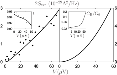
Figure 1: (a) Excess noise at $\nu=2/3$ (in unit of $10^{-29}$ ${\rm{A}}^{2}/{\rm{Hz}}$) as a function of $V$ for $T=10$ mK (corresponding voltage $V=T/e^{*}=2.6$ $\mu V$). Inset: transmission $t$ as given in Eq. (10) as a function of $V$ with $t(V=0)=0.95$. Diamonds represent the experimental data taken from Ref. Ofek09, , with courtesy of Moty Heiblum. (b) Same as in (a) but at $T=80$ mK. Inset: log-log plot of the total linear backscattering conductance (in unit of $G_{0}=e^{2}/2\pi$) as a function of temperature. Other parameters: $g_{\rm{c}}=1.6$, $g_{\rm{n}}=8.1$, $\omega_{\rm{c}}=5$ K, $\omega_{\rm{n}}=200$ mK, $\gamma_{2}/\gamma_{1}=0.20$, $\gamma_{1}^{2}/\omega_{c}^{2}=1.1\cdot 10^{-1}$.

The above results demonstrates that the value of the effective tunneling charge crucially depends on the external parameters such as temperature and voltage.

This point can be further analyzed by considering the temperature dependence of the effective charge at low voltages, $e^{*}V<T$. Fig. 2 shows ${e}^{\rm th}_{\rm{eff}}$, evaluated using the expression (15), for different values of the tunneling amplitude ratio $\gamma_{2}/\gamma_{1}$ between a bunch of two qps $(\gamma_{2})$ and a single qp $(\gamma_{1})$. At low temperatures, the effective charge corresponds to the $|p|=2$ agglomerate with ${e}^{\rm th}_{\rm{eff}}=\nu e$, while, increasing temperature, it reaches the single-qp value ${e}^{\rm th}_{\rm{eff}}=\nu e/|p|$. The crossover region between the two regimes is driven by $T^{*}$ which increases increasing the ratio of $\gamma_{2}/\gamma_{1}$.

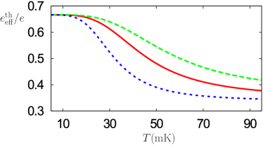
Figure 2: Effective charge, in unit of the electron charge $e$, as a function of temperature, for $\nu=2/3$ and different values of the ratio $\gamma_{2}/\gamma_{1}=0.1$ (blue, short-dashed), $0.2$ (red, straigth), $0.35$ (green, long-dashed). The corresponding crossover temperatures are $T^{*}=32$ mK, $42$ mK, $60$ mK respectively. The other parameters are as in Fig. 1.

We conclude the comparison with experiments by considering the effective charge for filling factor $\nu=2/5$ where experimental data are available. This case was discussed in Ref. Ferraro08, where model parameters were fixed by fitting the temperature dependence of the linear conductance. Here we focus on the temperature behavior of the effective charge.

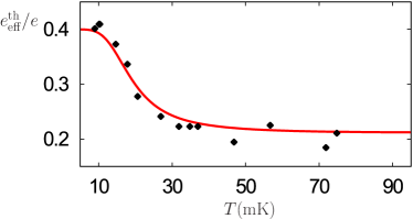
Figure 3: Effective charge, in unit of the electron charge $e$, as a function of temperature, for $\nu=2/5$. Diamonds represent the experimental data taken from Ref. Chung03, , with courtesy of Moty Heiblum. Parameters: $g_{\rm{c}}=3$, $g_{\rm{n}}=12$, $\omega_{\rm{c}}=5$ K, $\omega_{\rm{n}}=50$ mK, $\gamma_{2}/\gamma_{1}=0.65$, with $T^{*}=18$ mK.

Fig. 3 shows the evolution of ${e}^{\rm th}_{\rm{eff}}$ as a function of temperature. The agreement with the corresponding quantity measured in Ref. Chung03, (black diamonds) is very good and reinforces the crossover scenario of tunneling from single-qps to agglomerates at sufficiently low temperature. Note that for the above fit we used the parameters fixed in Ref. Ferraro08, for the linear conductance. They are however here expressed for the LW model with co-propagating neutral and charged modesFerraro08 .

V Conclusion

We proposed a minimal hierarchical model which fully explains recent experimental observations on excess noise at low temperatures and weak backscattering. The meaning of the effective charge and its temperature dependence was analyzed in comparison with the available experimental data. A quantitative analysis of the dependence of noise and effective charge on external parameters was performed. Evidence of neutral modes propagating with finite velocity and quantitative value of the corresponding bandwidth were extracted.

Our results show that the increasing of the effective charges, observed in experiments at extremely low temperatures for the Jain sequence, can be well explained in terms of the dominance of the $|p|$-agglomerates over the single-qp contribution. Only at sufficiently high energies the single-qp dominance is again recovered. We expect that the described crossover could be also relevant for other filling factors, outside of the Jain sequence, where anomalous increasing of the effective charges is also observed dolev10 .

As a final remark we note that within the analyzed geometry with a point-like scatterer we cannot shed light on the propagation direction of the neutral modes, but only on their presence. The fit of the experiments were done using the value $\xi={\rm{sgn}}(p)$ (LW model), which corresponds to a counter-propagating neutral mode for $\nu=2/3$ in accordance with recent observationsAveek10 . However, one could have fit as well the data in the other case with $\xi=-{\rm{sgn}}(p)$ (GFL model) with a co-propagating neutral mode for $\nu=2/3$, simply changing the interaction parameters (cf. Eq.(5)). Anyway, to have information on the direction of propagation one should consider more complicated geometries such as the four terminal steup recently addressed in experiments Aveek10 .

References

- (1) S. Das Sarma, A. Pinczuk Perspective in Quantum Hall Effects: Novel Quantum Liquid in Low-Dimensional Semiconductor Structures (Wiley, New York 1997).
- (2) R. B. Laughlin, Phys. Rev. Lett 50, 1395 (1983).
- (3) X. G. Wen, Phys. Rev. Lett. 64, 2206 (1990).
- (4) X. G. Wen, Phys. Rev. B 43, 11025 (1991).
- (5) X. G. Wen, Adv. Phys. 44, 405 (1995).
- (6) R. de Picciotto, M. Reznikov, M. Heiblum, V. Umansky, G. Bunin, and D. Mahalu, Nature 389, 162 (1997).
- (7) L. Saminadayar, D. C. Glattli, Y. Jin, and B. Etienne, Phys. Rev. Lett. 79, 2526 (1997).
- (8) Y. C. Chung, M. Heiblum, and V. Umansky, Phys. Rev. Lett 91, 216804 (2003).
- (9) A. Bid, N. Ofek, M. Heiblum, V. Umansky, and D. Mahalu, Phys. Rev. Lett. 103, 236802 (2009).
- (10) M. Dolev, Y. Gross, Y. C. Chung, M. Heiblum, V. Umansky, and D. Mahalu, Phys. Rev. B 81, 161303(R) (2010).
- (11) S. Roddaro, V. Pellegrini, F. Beltram, G. Biasiol, and L. Sorba, Phys. Rev. Lett. 93, 046801 (2004).
- (12) P. Fendley, A. W. W. Ludwig, and H. Saleur, Phys. Rev. Lett. 75, 2196 (1995).
- (13) B. Rosenow and B. I. Halperin, Phys. Rev. Lett. 88, 096404 (2002).
- (14) E. Papa and A. H. MacDonald, Phys. Rev. Lett. 93, 126801 (2004).
- (15) S. S. Mandal and J. K. Jain, Phys. Rev. Lett. 89, 096801 (2002).
- (16) K. Yang, Phys. Rev. Lett. 91, 036802 (2003).
- (17) I. L. Aleiner and L. I. Glazman, Phys. Rev. Lett. 72, 2935 (1994).
- (18) X. G. Wen and A. Zee, Phys. Rev. B 46, 2290 (1992).
- (19) C. L. Kane, M. P. A. Fisher, and J. Polchinski, Phys. Rev. Lett. 72, 4129 (1994).
- (20) C. L. Kane and M. P. A. Fisher, Phys. Rev. B 51, 13449 (1995).
- (21) A. Lopez and E. Fradkin, Phys. Rev. B 59, 15323 (1999).
- (22) A. Lopez and E. Fradkin, Phys. Rev B 63, 085306 (2001).
- (23) D. Ferraro, A. Braggio, M. Merlo, N. Magnoli, and M. Sassetti, Phys. Rev. Lett. 101, 166805 (2008).
- (24) M. Levin, B. I. Halperin, and B. Rosenow, Phys. Rev. Lett. 99, 236806 (2007).
- (25) D. E. Feldman and F. Li, Phys. Rev. B. 78, 161304 (2008).
- (26) B. J. Overbosch and C. Chamon, Phys. Rev. B 80, 035319 (2009).
- (27) A. Cappelli, L. S. Georgiev, and G. R. Zemba, J. Phys. A: Math. Theor. 42, 222001 (2009).
- (28) A. Cappelli, G. Viola, and G. R. Zemba, Ann. Phys. 325, 465 (2010).
- (29) D. Ferraro, A. Braggio, N. Magnoli, and M. Sassetti, New J. Phys. 12, 013012 (2010).
- (30) Z. X. Hu, E. H. Rezayi, X. Wan, and K. Yang, Phys. Rev. B 80, 235330 (2009).
- (31) G. Granger, J. P. Eisenstein, and J. L. Reno, Phys. Rev. Lett. 102, 086803 (2009).
- (32) B. Aveek, N. Ofek, H. Inoue, M. Heiblum, C. L. Kane, V. Umansky, and D. Mahalu, cond-mat/1005.5724 (unpublished).
- (33) B. Reulet, J. Senzier, and D. E. Prober, Phys. Rev. Lett. 91, 196601 (2003).
- (34) R. K. Lindell, J. Delahaye, M. A. Sillanpää, T. T. Heikkilä, E. B. Sonin, and P. J. Hakonen, Phys. Rev. Lett. 93, 197002 (2004).
- (35) Yu. Bomze, G. Gershon, D. Shovkun, L. S. Levitov, and M. Reznikov, Phys. Rev. Lett. 95, 176601 (2005).
- (36) B. Huard, H. Pothier, N. O. Birge, D. Esteve, X. Waintal, and J. Ankerhold, Ann. Phys. 16, 736 (2007).
- (37) A. V. Timofeev, M. Meschke, J. T. Peltonen, T. T. Heikkilä, and J. P. Pekola, Phys. Rev. Lett. 98, 207001 (2007).
- (38) G. Gershon, Yu. Bomze, E. V. Sukhorukov, and M. Reznikov, Phys. Rev. Lett. 101, 016803 (2008).
- (39) I. P. Levkivskyi and E. V. Sukhorukov, Phys. Rev. B 78, 045322 (2008).
- (40) I. P. Levkivskyi, A. Boyarsky, J. Frohlich, and E. V. Sukhorukov, Phys. Rev. B 80, 045319 (2009).
- (41) D. H. Lee and X. G. Wen, cond-mat/9809160 (unpublished).
- (42) C. Chamon, E. Fradkin, and A. Lopez, Phys. Rev. Lett. 98, 176801 (2007).
- (43) For one describes quasi-hole excitations not considered here.
- (44) W. P. Su, Phys. Rev. B 34, 1031 (1986).
- (45) J. Fröhlich, U. M. Studer, and E. Thiran, J. Stat. Phys. 86, 821 (1997).
- (46) K. Ino, Phys. Rev. Lett. 81, 5908 (1998).
- (47) R. Guyon, P. Devillard, T. Martin, and I. Safi, Phys. Rev. B 65, 153304 (2002).
- (48) T. Martin, Les Houches Session LXXXI ed. H. Bouchiat et al. (Elsevier, Amsterdam, 2005).
- (49) C. L. Kane and M. P. A. Fisher, Phys. Rev. Lett. 68, 1220 (1992).
- (50) L. S. Levitov and M. Reznikov, Phys. Rev. B 70, 115305 (2004).
- (51) A. Braggio, M. Sassetti, and B. Kramer, Phys. Rev. Lett. 87, 146802 (2001).
- (52) Note that our definition of noise differs from the one usually considered in experimental works (see e.g. Chung03, ; Ofek09, ) by a factor that has been properly taken into account in the analysis of the data. This definition is useful in order to avoid multiplicative factors in the expression of the current cumulants.
- (53) V. V. Ponomarenko and N. Nagaosa, Phys. Rev. B 60, 16865 (1999).
- (54) F. Dolcini, B. Trauzettel, I. Safi, and H. Grabert, Phys. Rev. B 71, 165309 (2005).