Spectral analysis of resonant x-ray scattering in CeB₆
under an external magnetic field

Abstract

We study the resonant x-ray scattering (RXS) spectra of CeB₆ in an antiferroquadrupole (AFQ) ordering phase, near the Ce $L_{3}$ edge under the applied magnetic field $\textbf{H}\parallel(\overline{1},1,0)$. On the basis of a localized electron model equipped with a mechanism that the RXS signal is brought about by the intra-atomic Coulomb interaction in Ce, we calculate the RXS spectra. The obtained spectra exhibit two contributions around the electric dipole ($E$1) and quadrupole ($E$2) positions, and differ drastically when the orientation of H is reversed. The difference is brought about by the cross terms between the even-rank AFQ and magnetic-induced odd-rank contributions. At the $E$1 region, the relevant cross term is the one within the $E$1 process, while at the $E$2 region, they are ones within the $E$2 process and between the $E$1 and $E$2 processes. These findings capture the characteristic features the recent experimental data show, and provide a strong support and information of the field-induced multipole orderings. We also evaluate the RXS spectra near the $L_{2}$ edge. Though the results show no $E$2 contribution, we find that the intensity around the $E$1 transition, which is as large as that at the $L_{3}$ edge, can be detected experimentally.

I Introduction

Numerous and intensive research activities have been concentrated in the field of the $f$-electron systems where mutual interplay of charge, spin, and orbital degrees of freedom produces a rich variety of physical properties characterizing the strongly correlated electron systems. Among a large number of interests, the materialization of the multipolar ordering phase in these systems is one of the most fascinating topics to be addressed.Santini et al. (2009); Kuramoto et al. (2009)

Resonant x-ray scattering (RXS) is one of the most promising probes to observe experimental evidences of the multipole order with rank higher than two. A tensorial nature of the scattering amplitude helps our understanding of the experimental result.Hannon et al. (1988); Blume (1994); Lovesey et al. (2005); Dmitrienko et al. (2005) However, an analysis based merely on the symmetrical consideration of the tensorial nature does not answer the origin of the observed RXS signals. For instance, when the RXS signals were detected at the Mn $K$-edge in the orbital ordering phase of manganites. Murakami et al. (1998a, b) There was a controversy on what brought about the observed signals. In the electric dipole ($E$1) transition, the $K$-edge signals reflect the anisotropic charge distribution of the $4p$ states, which form bands. Such an anisotropy may be given rise to by the distortion of the lattice or by the underlying ordering pattern of the $3d$ electrons through the intra-atomic Coulomb interaction.Ishihara and Maekawa (1998) We call the latter as the "Coulomb mechanism". Extensive investigations have revealed that the observed intensities were originated from the lattice distortion.Elfimov et al. (1999); Benfatto et al. (1999); Takahashi et al. (1999) Since the $4p$ states of transition metals are rather extended in space, this result is quite reasonable. It is now recognized that the same mechanism is working on the RXS in other transition-metal compounds such as YTiO₃ and YVO₃.Di Matteo (2009); Takahashi and Igarashi (2001, 2002)

The situation is different for RXS near the $L$-edge in rare-earth compounds, since the $4f$ states are so localized in space that the lattice distortion associated with multipole ordering is expected to be much smaller than that in transition-metal compounds. In CeB₆, the antiferroquadrupolar (AFQ) ordering phase is inferred from various indirect observations such as macroscopic measurements, resonance methods, neutron scattering, and so on.Takigawa et al. (1983); Effantin et al. (1985); Terzioglu et al. (2001); Zaharko et al. (2003); Schenck et al. (2004); Plakhty et al. (2005) The most direct evidence of the AFQ order is provided by the RXS experiment by Nakao et al.Nakao et al. (2001) and Yakhou et al., Yakhou et al. (2001) who have succeeded in detecting the RXS signal at the Ce $L_{3}$ edge at an AFQ Bragg spot $\textbf{G}=\left(\frac{1}{2},\frac{1}{2},\frac{1}{2}\right)$. Later, another experimental support was given by Tanaka et al. from the non-resonant x-ray Thomson scatteing (NRXTS) study which detected directly an evidence of the aspherical charge density.Tanaka et al. (2004) Note that no lattice distortionis are observed in this material.Akatsu et al. (2003); Sikora et al. (2005)

In our previous papers, we have calculated microscopically the RXS spectra on the basis of a localized electron picture which relies on the Coulomb mechanism, and have obtained the spectra in agreement with the experiments. Nagao and Igarashi (2001); Igarashi and Nagao (2002) In addition, invoking the same theoretical framework elaborated in Refs. Nagao and Igarashi, 2001 and Igarashi and Nagao, 2002, we have calculated the NRXTS intensities on the AFQ Bragg spots. Our result has reproduced well the relative intensities of RXS and NRXTS and a Fano-dip like structure at $\textbf{G}=\left(\frac{5}{2},\frac{3}{2},\frac{3}{2}\right)$, Nagao and Igarashi (2003) in accordance with the Yakhou et al.’s data.Yakhou et al. (2001)

It is predicted that the applied magnetic field induces the antiferro-octupole ordering in CeB₆,Shiina et al. (1997, 1998) which could be detected by RXS and neutron scatteringKuwahara et al. (2007) measurements. Matsumura et al. have recently succeeded in detecting the octupole ordering induced by the applied magnetic field via RXS.Matsumura et al. (2009) By using different experimental settings examined before,Nakao et al. (2001); Yakhou et al. (2001) they observed the RXS spectra near the Ce $L_{3}$ edge at $\textbf{G}=\left(\frac{3}{2},\frac{3}{2},\frac{1}{2}\right)$ under the applied field along $\textbf{H}\parallel(\overline{1},1,0)$ in the AFQ phase. Their data illustrate three notable features. First, in addition to main peak of the $E$1 transition around 5724 eV, the spectra show a small peak of the electric quadrupole ($E$2) transition around 5718 eV when the field is in the plus direction ($+\textbf{H}$). This finding makes a remarkable contrast with the previous RXS data where the $E$2 peak is practically absent both experimentally and theoretically.Nakao et al. (2001); Yakhou et al. (2001); Nagao and Igarashi (2001); Igarashi and Nagao (2002) Second, when the orientation of the applied field is reversed, the spectral shape drastically changes. That is, the small peak around the $E$2 position becomes obscure when the field is in the minus direction ($-\textbf{H}$). Third, the peak intensity at the $E$1 peak varies in certain amount when the direction of H is reversed. Note that although the final feature was not emphasized in Ref. Matsumura et al., 2009, they confirmed that the difference actually exists, in particular, for the field strength approximately larger than 2 $T$.com (a)

These features were analyzed to originate from the cross terms between the contributions of primary AFQ (even rank) order parameters and those of field-induced (odd rank) order parameters. The purpose of this paper is to elucidate those observations by analyzing quantitatively the spectra from a microscopic standpoint beyond qualitative one based merely on the symmetry consideration. Lovesey (2002) Developing our previous treatment,Nagao and Igarashi (2001); Igarashi and Nagao (2002); Nagao and Igarashi (2003) we find that the field dependence comes from the interference effect between the even rank and odd rank signals. Some of them come from the terms within the $E$1 process and within the $E$2 process, while others come from the terms between the $E$1 and $E$2 processes. Since the field-induced octupole ordering, for example, gives rise to the third order rank signal, the information of octupole ordering could be extracted from the field dependence of the spectra.

For numerical calculation, we adopt the same model and parameter settings to the previous works as possible as we can to keep continuity of the research. We obtain the spectra reproducing semiquantitatively the three features the experiment had revealed. Note that the ‘fast collision approximation’, which is widely used to analyze the spectra, is insufficient to discuss the field dependence, since it predicts no field dependence of the main peak intensity. Finally, we find that the RXS spectrum at the Ce $L_{2}$ edge has enough intensity to be detected experimentally.

This paper is organized as follows. In Sec. II, we introduce a theoretical framework to investigate the RXS intensity in the localized electron systems. In Sec. III, we briefly summarize a model Hamiltonian which describes the initial state and used in our previous works, and explain the mean field solution of the Hamiltonian. Also the intermediate states of the scattering processes are presented. Numerical results of the calculated RXS spectra are shown in Sec. IV with comparisons with the experimental results. The last section is devoted to concluding remarks.

II Theoretical Framework

II.1 Scattering amplitude

RXS is described as a second order optical process: photon with frequency $\omega$, wave number k, and polarization $\mu$ ($=\sigma$ or $\pi$) is diffracted by the sample into the state with the same frequency $\omega$, wave number $\textbf{k}^{\prime}$, and polarization $\mu^{\prime}$ ($=\sigma^{\prime}$ or $\pi^{\prime}$). The amplitude is approximated by a sum of the contributions from each Ce ion, which can be written as

$$F(\textbf{k},\mbox{\boldmath{$\epsilon$}};\textbf{k}^{\prime},\mbox{\boldmath{$\epsilon$}}^{\prime}:\omega)=\sum_{n=1,2}f_{n}(\textbf{k},\mbox{\boldmath{$\epsilon$}};\textbf{k}^{\prime},\mbox{\boldmath{$\epsilon$}}^{\prime}:\omega),$$ (1)

where $f_{n}$ stands for the scattering amplitude of the $En$-$En$ transition and electric $2^{n}$-th pole process is abbreviated to $En$. We omit the contributions from the terms like $En$-$Em$ with $n\neq m$ since we restrict our attention to centrosymmetric system. In this context, the $En$-$En$ transition is simply called as the $En$ transition hereafter. The $En$ amplitude is written as

$$f_{n}(\textbf{k},\mbox{\boldmath{$\epsilon$}};\textbf{k}^{\prime},\mbox{\boldmath{$\epsilon$}}^{\prime}:\omega)\propto\frac{1}{\sqrt{N}}\sum_{j}\textrm{e}^{-i\textbf{G}\cdot\textbf{r}_{j}}M_{n}(j:\textbf{k},\mbox{\boldmath{$\epsilon$}};\textbf{k}^{\prime},\mbox{\boldmath{$\epsilon$}}^{\prime}:\omega),$$ (2)

where $M_{n}(j:\textbf{k},\mbox{\boldmath{$\epsilon$}};\textbf{k}^{\prime},\mbox{\boldmath{$\epsilon$}}^{\prime}:\omega)$ represents the RXS amplitude at site $j$ with position vector $\textbf{r}_{j}$. The number of Ce site is denoted as $N$. Scattering vector G is defined by $\textbf{k}^{\prime}-\textbf{k}$. Note that the above expressions aimed for absolute zero temperature are easily extended for a treatment of finite temperature ($T$) case by multiplying probability $p_{j,m}$ to $M_{n}(j:\textbf{k},\mbox{\boldmath{$\epsilon$}};\textbf{k}^{\prime},\mbox{\boldmath{$\epsilon$}}^{\prime}:\omega)$ and summing over $m$. Here $p_{j,m}$ is proportional to the Boltzmann factor $\textrm{e}^{-E_{j,m}/T}$ with $E_{j,m}$ being the energy of the $m$-th eigenstate at site $j$. For simplicity, we proceed the formulation for $T=0$, though our numerical calculations in Sec. IV will be those for finite temperatures.

The $E$1 amplitude is

$$M_{1}(j:\mbox{\boldmath{$\epsilon$}};\mbox{\boldmath{$\epsilon$}}^{\prime}:\omega)=\sum_{\mu,\mu^{\prime}=1}^{3}\epsilon_{\mu}^{\prime}\epsilon_{\mu^{\prime}}\sum_{\Lambda}\frac{\langle 0|x_{\mu,j}|\Lambda\rangle\langle\Lambda|x_{\mu^{\prime},j}|0\rangle}{\hbar\omega-(E_{\Lambda}-E_{0})+i\Gamma},$$ (3)

where $|0\rangle$ denotes the ground state with eigenenergy $E_{0}$, while $|\Lambda\rangle$ denotes the intermediate state with eigenenergy $E_{\Lambda}$. The lifetime broadening width of the core hole is represented by $\Gamma$ and it is fixed to be 1.5 eV in this work. The dipole operators $x_{\mu,j}$ are described as $x_{j},y_{j}$, and $z_{j}$ for $\mu=1,2$, and $3$, respectively, in the coordinate system fixed to the crystal axes with the origin located at the center of site $j$. The $E$2 amplitude is

$$M_{2}(j:\textbf{k},\mbox{\boldmath{$\epsilon$}};\textbf{k}^{\prime},\mbox{\boldmath{$\epsilon$}}^{\prime}:\omega) = \frac{k^{2}}{9}\sum_{\mu,\mu^{\prime}=1}^{5}q_{\mu}(\hat{\textbf{k}}^{\prime}\cdot\mbox{\boldmath{$\epsilon$}}^{\prime})q_{\mu^{\prime}}(\hat{\textbf{k}}\cdot\mbox{\boldmath{$\epsilon$}})$$ (4)

$$\times \sum_{\Lambda}\frac{\langle 0|\tilde{z}_{\mu,j}|\Lambda\rangle\langle\Lambda|\tilde{z}_{\mu^{\prime},j}|0\rangle}{\hbar\omega-(E_{\Lambda}-E_{0})+i\Gamma},$$

where factors $q_{\mu}(\hat{\textbf{k}}^{\prime}\cdot\mbox{\boldmath{$\epsilon$}}^{\prime})$ and $q_{\mu^{\prime}}(\hat{\textbf{k}}\cdot\mbox{\boldmath{$\epsilon$}})$ with $\hat{\textbf{k}}^{\prime}=\textbf{k}^{\prime}/|\textbf{k}^{\prime}|$ and $\hat{\textbf{k}}=\textbf{k}/|\textbf{k}|$ are defined as a second-rank tensor,

$$q_{\mu}(\textbf{A},\textbf{B})=\left\{\begin{array}[]{ll}\frac{\sqrt{3}}{2}(A_{x}B_{x}-A_{y}B_{y})&\textrm{for}\ \mu=1,\\ \frac{1}{2}(3A_{z}B_{z}-\textbf{A}\cdot\textbf{B})&\textrm{for}\ \mu=2,\\ \frac{\sqrt{3}}{2}(A_{y}B_{z}+A_{z}B_{y})&\textrm{for}\ \mu=3,\\ \frac{\sqrt{3}}{2}(A_{z}B_{x}+A_{x}B_{z})&\textrm{for}\ \mu=4,\\ \frac{\sqrt{3}}{2}(A_{x}B_{y}+A_{y}B_{x})&\textrm{for}\ \mu=5.\\ \end{array}\right.$$ (5)

Note that the quadrupole operator $\tilde{z}_{\mu,j}$ is expressed as $\tilde{z}_{\mu,j}=q_{\mu}(\textbf{r}_{j},\textbf{r}_{j})$, and the subscripts $\mu=1,2,3,4$, and $5$ for rank two quantity specify the Cartesian components $x^{2}-y^{2},3z-r^{2},yz,zx$, and $xy$, respectively.

In general, the evaluation of the scattering amplitude $M_{n}$ tends to be a formidable task, since the intermediate states of the scattering process are difficult to calculate. However, there exist several cases in which the evaluation of the scattering amplitude becomes easy. For instance, by replacing the energy denominators in $M_{n}$ with a single oscillator, the amplitudes are reduced into compact forms.Luo et al. (1993); Lovesey et al. (2005) This treatment is called as ’fast collision approximation’. Here, we adopt an another treatment, in which the Hamiltonian describing the intermediate states is assumed to preserve a spherical symmetry. For only the $f$ states concerned, this assumption is justified when the crystal electric field (CEF) and the intersite interaction are negligible compared with the intra-atomic Coulomb and the spin-orbit interactions in the intermediate states. Analyses based on this framework gave good results in many localized $f$-electron systems.Nagao and Igarashi (2005, 2006, 2008) In the present case, this assumption seems applicable to the intermediate state of the $E$2 transition, while the applicability is not clear for the intermediate states of the $E$1 transition, since the $5d$ bands are involved. In this paper, assuming the same $5d$-DOS for the $e_{g}$ and $t_{2g}$ symmetries, we preserve the spherical symmetry in the intermediate states to calculate the RXS spectra. This assumption is justified later in our semi-quantitative analysis, since the RXS spectra are not sensitive to the shape and the fillingness of the $5d$ DOS.

Within the present scheme, the RXS scattering amplitudes are expressed in neat forms suitable to discuss field dependence. For the $E$1 process, the scattering amplitude at a single site is

$$M_{1}(\mbox{\boldmath{$\epsilon$}};\mbox{\boldmath{$\epsilon$}}^{\prime}:\omega)=\sum_{\nu=0}^{2}\alpha_{1}^{(\nu)}(\omega)\sum_{\mu=1}^{2\nu+1}P_{1,\mu}^{(\nu)}(\mbox{\boldmath{$\epsilon$}},\mbox{\boldmath{$\epsilon$}}^{\prime})\langle 0|z_{\mu}^{(\nu)}|0\rangle,$$ (6)

where $z_{\mu}^{(\nu)}$ is operator equivalence of mutipole moment of the component $\mu$ with rank $\nu$. For rank zero, $z_{1}^{(0)}=1$, and for rank one, $z_{\mu}^{(1)}$’s are $J_{x},J_{y}$, and $J_{z}$ with $\mu=1,2$, and $3$, respectively. For rank two, quadrupole operator is represented by $z_{\mu}^{(2)}=q_{\mu}(\textbf{J},\textbf{J})$. The energy profile of rank $\nu$ contribution is denoted as $\alpha_{1}^{(\nu)}(\omega)$, whose explicit form is found in Ref. Nagao and Igarashi, 2005. The geometrical factors are given as follows: for rank zero, $P_{1,1}^{(0)}(\mbox{\boldmath{$\epsilon$}},\mbox{\boldmath{$\epsilon$}}^{\prime})$$=$ $\mbox{\boldmath{$\epsilon$}}^{\prime}\cdot\mbox{\boldmath{$\epsilon$}}$, for rank one, $P_{1,\mu}^{(1)}(\mbox{\boldmath{$\epsilon$}},\mbox{\boldmath{$\epsilon$}}^{\prime})$$=$ $-i(\mbox{\boldmath{$\epsilon$}}^{\prime}\times\mbox{\boldmath{$\epsilon$}})_{\mu}$, and for rank two, $P_{1,\mu}^{(2)}(\mbox{\boldmath{$\epsilon$}},\mbox{\boldmath{$\epsilon$}}^{\prime})$$=$ $q_{\mu}(\mbox{\boldmath{$\epsilon$}}^{\prime},\mbox{\boldmath{$\epsilon$}})$. Note that we have omitted the subscript specifying the site and do so hereafter. For the $E$2 process, the scattering amplitude at a single site is

$$M_{2}(\textbf{k},\mbox{\boldmath{$\epsilon$}};\textbf{k}^{\prime},\mbox{\boldmath{$\epsilon$}}^{\prime}:\omega) = \frac{k^{2}}{9}\sum_{\nu=0}^{4}\alpha_{2}^{(\nu)}(\omega)\sum_{\mu=1}^{2\nu+1}P_{2,\mu}^{(\nu)}(\mbox{\boldmath{$\epsilon$}},\mbox{\boldmath{$\epsilon$}}^{\prime},\hat{\textbf{k}},\hat{\textbf{k}}^{\prime})$$ (7)

$$\times \langle 0|z_{\mu}^{(\nu)}|0\rangle,$$

where $P_{2,\mu}^{(\nu)}(\mbox{\boldmath{$\epsilon$}},\mbox{\boldmath{$\epsilon$}}^{\prime},\hat{\textbf{k}},\hat{\textbf{k}}^{\prime})$ is the geometrical factor of the component $\mu$ with rank $\nu$. The definitions of $z_{\mu}^{(\nu)}$ with rank $\nu$ higher than three and $P_{2,\mu}^{(\nu)}(\mbox{\boldmath{$\epsilon$}},\mbox{\boldmath{$\epsilon$}}^{\prime},\hat{\textbf{k}},\hat{\textbf{k}}^{\prime})$ are given in Ref. Nagao and Igarashi, 2006.com (b) These formulae look similar to those derived in literatures, mainly employing the fast collision approximation.Hannon et al. (1988); Luo et al. (1993); Carra and Thole (1994); Hill and McMorrow (1996); Lovesey et al. (2005) Our treatment, however, is convenient when spectral analysis is needed since the energy profiles in Eqs. (6) and (7) are correctly included. In the next section, we shall see Eq. (7) is strictly applicable to describing the $E$2 process at the Ce $L_{2,3}$ edges, while Eq. (6) is approximately valid to express the $E$1 process.

II.2 Intensity of the difference spectrum

We investigate how the RXS intensity changes when the orientation of the applied field is reversed. For antiferro-type scattering vector G, the factor $\textrm{e}^{-i\textbf{G}\cdot\textbf{r}_{j}}$ appeared in Eq. (2) gives $+1$ or $-1$ depending on the kind of sublattice the site $j$ belonging to. By substituting Eqs. (2), (6), and (7) into Eq. (1), we obtain the total amplitude of RXS with H along a certain direction as

$$F(\textbf{k},\mbox{\boldmath{$\epsilon$}};\textbf{k}^{\prime},\mbox{\boldmath{$\epsilon$}}^{\prime}:\omega)\propto\sqrt{N}\left[i\alpha_{1}^{(1)}(\omega)Z_{1}^{(1)}+\alpha_{1}^{(2)}(\omega)Z_{1}^{(2)}\right.$$

$$\left.+i\alpha_{2}^{(1)}(\omega)Z_{2}^{(1)}+\alpha_{2}^{(2)}(\omega)Z_{2}^{(2)}+i\alpha_{2}^{(3)}(\omega)Z_{2}^{(3)}\right],$$ (8)

where the term $\alpha_{2}^{(4)}(\omega)Z_{2}^{(4)}$ is omitted since it is absorbed into $\alpha_{2}^{(2)}(\omega)Z_{2}^{(2)}$ in the present case of CeB₆.Shiina et al. (1997) Here, use has been made of a new quantity

$$Z_{n}^{(\nu)}=\left\{\begin{array}[]{rl}\sum_{\mu=1}^{2\nu+1}P_{n,\mu}^{(\nu)}(\mbox{\boldmath{$\epsilon$}},\mbox{\boldmath{$\epsilon$}}^{\prime})\langle z_{\mu}^{(\nu)}\rangle&\textrm{for}\ \ \nu=\textrm{even}\\ -i\sum_{\mu=1}^{2\nu+1}P_{n,\mu}^{(\nu)}(\mbox{\boldmath{$\epsilon$}},\mbox{\boldmath{$\epsilon$}}^{\prime})\langle z_{\mu}^{(\nu)}\rangle&\textrm{for}\ \ \nu=\textrm{odd}\\ \end{array}\right.,$$ (9)

where the staggered moment is referred to as $\langle z_{\mu}^{(\nu)}\rangle$. It is related to the sublattice moments as $\langle z_{\mu}^{(\nu)}\rangle$$=$ $\langle 0|z_{\mu}^{(\nu)}|0\rangle_{A}$$=$ $-\langle 0|z_{\mu}^{(\nu)}|0\rangle_{B}$ where the subscripts $A$ and $B$ distinguish the sublattices. We emphasize that $\{Z_{n}^{(\nu)}\}$’s are real quantities. Note that only staggered components of the multipole operators contribute to the amplitude with the antiferro-type G.

The RXS intensity $I(\omega,\textbf{H})$ is given by $|F(\textbf{k},\mbox{\boldmath{$\epsilon$}};\textbf{k}^{\prime},\mbox{\boldmath{$\epsilon$}}^{\prime}:\omega)|^{2}$. When the direction of the applied field is reversed, $Z_{1}^{(\nu)}$ and $Z_{2}^{(\nu)}$ having odd $\nu$ reverse their signs, while those having even $\nu$ remain unchanged. Therefore, the amplitude for $-\textbf{H}$ is expressed by the quantities for $+\textbf{H}$. Then, the total intensities are expressed as

$$I(\omega,\pm\textbf{H})\propto\left|\alpha_{1}^{(2)}(\omega)Z_{1}^{(2)}+\alpha_{2}^{(2)}(\omega)Z_{2}^{(2)}\right.$$

$$\left.\pm i\{\alpha_{1}^{(1)}(\omega)Z_{1}^{(1)}+\alpha_{2}^{(1)}(\omega)Z_{2}^{(1)}+\alpha_{2}^{(3)}(\omega)Z_{2}^{(3)}\}\right|^{2}.$$ (10)

The difference spectrum is defined as

$$\Delta I(\omega)\equiv\frac{I(\omega,+\textbf{H})-I(\omega,-\textbf{H})}{2}.$$ (11)

The spectrum $\Delta I(\omega)$ produces non-zero contribution when cross terms between the amplitude with odd rank and that with even rank remains finite. By substituting (10) into Eq. (11), we can classify such cross terms into three categories:

$$\Delta I(\omega) = \Delta I_{E1E2}+\Delta I_{E1E1}+\Delta I_{E2E2},$$ (12)

$$\Delta I_{E1E2} \equiv 2Z_{1}^{(1)}Z_{2}^{(2)}\textrm{Im}[\{\alpha_{1}^{(1)}(\omega)\}^{\star}\alpha_{2}^{(2)}(\omega)]$$ (13)

$$+ 2Z_{1}^{(2)}Z_{2}^{(1)}\textrm{Im}[\{\alpha_{2}^{(1)}(\omega)\}^{\star}\alpha_{1}^{(2)}(\omega)]$$

$$+ 2Z_{1}^{(2)}Z_{2}^{(3)}\textrm{Im}[\{\alpha_{2}^{(3)}(\omega)\}^{\star}\alpha_{1}^{(2)}(\omega)],$$

$$\Delta I_{E1E1} \equiv 2Z_{1}^{(1)}Z_{1}^{(2)}\textrm{Im}[\{\alpha_{1}^{(1)}(\omega)\}^{\star}\alpha_{1}^{(2)}(\omega)],$$ (14)

$$\Delta I_{E2E2} \equiv 2Z_{2}^{(1)}Z_{2}^{(2)}\textrm{Im}[\{\alpha_{2}^{(1)}(\omega)\}^{\star}\alpha_{2}^{(2)}(\omega)]$$ (15)

$$+ 2Z_{2}^{(3)}Z_{2}^{(2)}\textrm{Im}[\{\alpha_{2}^{(3)}(\omega)\}^{\star}\alpha_{2}^{(2)}(\omega)],$$

where $\textrm{Im}[X]$ stands for imaginary part of $X$.

Before showing numerical results of the RXS spectra, we comment on an outcome expected from the fast collision approximation, in which the energy denominators in Eqs. (3) and (4) are factored out of the summation over the intermediate states and replaced by a single oscillator.Luo et al. (1993); Lovesey et al. (2005) As a consequence, the energy profile $\alpha_{n}^{(\nu)}(\omega)$ loses its $\nu$ dependence, say $\alpha_{n}(\omega)$. Then, $\Delta I_{E1E1}(\omega)$ and $\Delta I_{E2E2}(\omega)$ become zero, and $\Delta I_{E1E2}(\omega)$ alone remains as

$$\Delta I_{E1E2}(\omega) = 2[Z_{1}^{(1)}Z_{2}^{(2)}-Z_{1}^{(2)}(Z_{2}^{(1)}+Z_{2}^{(3)})]$$ (16)

$$\times\textrm{Im}[\{\alpha_{1}(\omega)\}^{\star}\alpha_{2}(\omega)].$$

This expression is what Matsumura et al. have used in their analysis.Matsumura et al. (2009)

III Initial and intermediate states

Cerium hexaboride is believed to show an AFQ ordering phase in the temperature range $T_{\textbf{N}}\leq T\leq T_{\textrm{Q}}$ with $T_{\textrm{N}}=2.3$ KEffantin et al. (1985); Zaharko et al. (2003) and $T_{\textrm{Q}}=3.3$ K under no applied magnetic field.Komatsubara et al. (1980); Effantin et al. (1985); Yakhou et al. (2001) It shows a simple cubic structure (CsCl-type, P${}_{m\overline{3}m}$) with lattice constant $a$ being $4.14\textrm{\AA}$. In CeB₆, Ce is trivalent in the $f^{1}$ configuration forming a sextet term ${}^{2}\textrm{F}_{\frac{5}{2}}$. Under the cubic symmetry CEF, the sextet splits into a $\Gamma_{7}$ doublet and a $\Gamma_{8}$ quartet. The latter is the lowest energy state. Since the energy splitting between them is on the order of 530 K,Zirngiebl et al. (1984) the $\Gamma_{8}$ quartet alone is sufficient for investigating low-temperature phenomena. Within the $\Gamma_{8}$ basis under the $O_{h}$ symmetry, multipolar operators with rank one, two, and three are active. In the following, we introduce a model Hamiltonian defined in a subspace spanned by $\Gamma_{8}$ basis.

III.1 Model Hamiltonian

In order to prepare the initial (or ground) state of the AFQ state in CeB₆, we adopt the model Hamiltonian utilized in our previous works.Nagao and Igarashi (2001); Igarashi and Nagao (2002); Nagao and Igarashi (2003) It is originally introduced by OhkawaOhkawa (1985) and extended by Shiina et al.Shiina et al. (1997) It is derived on the basis of the RKKY interaction and a possibility of the anisotropic RKKY interaction is discarded for simplicity.Schlottmann (2000) The Hamiltonian is

$$\hat{H} = \frac{D}{4}\sum_{\langle i,j\rangle}\left[(1+\delta)\sum_{\mu=3}^{5}O_{\mu,i}O_{\mu,j}+\frac{1}{16}\sum_{\mu=1}^{2}O_{\mu,i}O_{\mu,j}\right]$$ (17)

$$+ D\sum_{\langle i,j\rangle}\left[\tau_{i}^{y}\tau_{j}^{y}+\mbox{\boldmath{$\sigma$}}_{i}\cdot\mbox{\boldmath{$\sigma$}}_{j}+\mbox{\boldmath{$\eta$}}_{i}\cdot\mbox{\boldmath{$\eta$}}_{j}+\mbox{\boldmath{$\zeta$}}_{i}\cdot\mbox{\boldmath{$\zeta$}}_{j}\right]$$

$$+ g\mu_{\textrm{B}}\sum_{i}\textbf{J}_{i}\cdot\textbf{H},$$

where operator equivalence of quadrupole moment is defined as $O_{\mu}=q_{\mu}(\textbf{J},\textbf{J})$. The second line of Eq. (17) describes the interactions between dipole and octupole moments, and the definitions of the symbols appeared in this line are found, e.g., in Refs. Shiina et al., 1997 and Igarashi and Nagao, 2002. The sum on $\langle i,j\rangle$ runs over nearest neighbor Ce pairs. The last line in Eq. (17) stands for the Zeeman term with $g$-factor being $6/7$. Note that, by choosing parameter $\delta$ positive, this Hamiltonian favors the AFQ order of three components belonging to the $\Gamma_{5}$ basis ($O_{yz},O_{zx}$, and $O_{xy}$). The parameter $\delta$ is fixed as $\delta=0.2$. The coupling constant is chosen so as to reproduce the value of $T_{\textrm{Q}}$ in the absence of magnetic field.

III.2 Mean field solutions and the initial states

Figure 1: H-dependence of the staggered moments at $T=1.65$ K. Bold solid and broken lines are $\langle O_{-1,1,0}\rangle$ and $\langle J_{z}\rangle$, respectively. Thin solid and broken lines denote $\langle t_{z}^{\alpha}\rangle=\langle T_{z}^{\alpha}\rangle/\sqrt{50}$ and $\langle t_{xyz}\rangle=\langle T_{xyz}\rangle/(45/2\sqrt{5})$.

We apply the mean field approximation to the Hamiltonian. Under the influence of the external field H along $(h,k,\ell)$ direction, the mean field solution gives a ground state of the primary order parameter $\langle O_{hk\ell}\rangle=\langle(hO_{yz}+kO_{zx}+\ell O_{xy})\rangle/\sqrt{h^{2}+k^{2}+\ell^{2}}$. The quadrupole ordering temperature $T_{\textrm{Q}}^{0}$ in the zero field limit is given by 3.3 K for $D=0.458$ K. The field induces another ranks and/or another components of multipole order parameters depending on the direction of the applied field.Shiina et al. (1997, 1998) In the case of $\textbf{H}\parallel(\overline{1},1,0)$ adopted by Matsumura et al.,Matsumura et al. (2009) three antiferro-type of the secondary order parameters, a dipole component $J_{z}$ and octupole components $T_{xyz}$ and $T_{z}^{\alpha}$, are induced. Note that the definitions of $T_{xyz}(=z_{1}^{(3)})$ and $T_{z}^{\alpha}(=z_{4}^{3)}$) are given in Ref. Nagao and Igarashi, 2006. The field dependences of these order parameters are shown in Fig. 1 for $T=T_{\textrm{Q}}^{0}/2=1.65$ K. Since $|\textbf{H}|$-dependence of the order parameters, both primary and induced ones, become mild beyond $|\textbf{H}|\simeq 1$T, we will fix the field strength $|\textbf{H}|=2$ T throughout the present work. This choice of the magnitude of H enables us to avoid complication concerning the problem of domain population, which is known to exist when the applied field is much smaller as seen in Fig. 2 of Ref. Matsumura et al., 2009. Finally, note that though many more order parameters are induced in ferro-type alignments, we do not mention them since they have no contribution on the RXS intensity at the antiferro-type scattering vector now addressed.

III.3 Intermediate states

The intermediate states of RXS near the Ce $L_{2,3}$ absorption edges include excitations of an electron from core $2p$ states at a Ce site into the $5d$ and $4f$ states in the $E$1 and $E$2 processes, respectively. Since the $5d$ states form not levels but conduction bands, we need a model of the density of states (DOS) of them. In order to keep continuity from our previous work, we employ the same $5d$ DOS used before.Nagao and Igarashi (2001); Igarashi and Nagao (2002); Nagao and Igarashi (2003) The $5d$ DOS, $\rho^{5d}(x)$, is assumed to be

$$\rho^{5d}(x)=\left\{\begin{array}[]{ll}0.008x+0.04,&-5<x<0,\\ 0.01x+0.04,&0<x<8\\ -0.0277x+0.342,&8<x<12.33,\end{array}\right.$$ (18)

where $x$ is measured in units of eV with $x=0$ corresponding to the Fermi level. Total number of the occupied $5d$ electron per Ce site is set to be unity. We disregard the dependence on the $5d$ states $x^{2}-y^{2},3z^{2}-r^{2},yz,zy$, and $xy$. These settings are justified later in our semi-quantitative analysis, since the RXS spectra are not sensitive to the shape and the fillingness of the $5d$ DOS. Figure 2 shows a schematic view of the RXS processes and the shape of the $5d$ DOS.

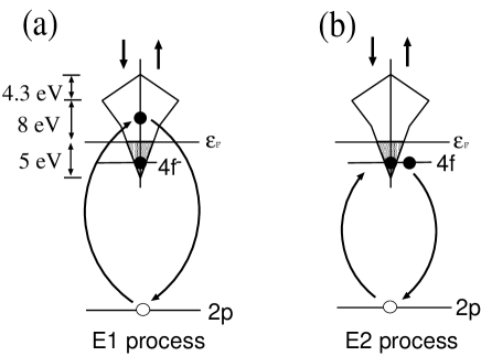
Figure 2: Schematic diagrams of two RXS processes at the Ce $L_{2}$ and $L_{3}$ edges: (a) $E$1 process; (b) $E$2 process The $5d$ DOS is schematically exhibited in the upper part of the figure and arrows indicate spin of the $5d$ states.

III.3.1 $E$1 process

As explained above, the $E$1 transition at the $L_{2,3}$ edges consists of that between the $2p$ and $5d$ states. We consider the resolvent $[\hbar\omega-H_{int}]^{-1}$, where $H_{int}$ is the Hamiltonian spanned in the configuration involving one $4f$ electron, one $2p$ core hole, and one excited electron in the $5d$ band. First, we solve an eigenvalue problem considering the Coulomb interaction between the $4f$ and $2p$ core hole as well as the spin-orbit interaction of them at the central site. Let the eigenvalue and the eigenstate be $E_{\lambda}$ and $|\lambda\rangle$, respectively. In this work, the Slater integrals and the spin-orbit interaction parameters needed to evaluate the Coulomb and spin-orbit interactions are calculated for Ce³⁺ atom within the Hartree-Fock (HF) approximation.Cowan (1981) The obtained off-diagonal and diagonal values of the Slater integrals are multiplied by factors 0.8 and 0.25, respectively, taking the screening effect into account. Then, the presence of the $5d$ electron is treated as a scattering problem. The problem is described by an inverse matrix problem symbolically summarized below:

$$\left(\frac{1}{\hbar\omega-H_{int}+i\gamma}\right)_{d\lambda,d^{\prime}\lambda^{\prime}}$$ (19)

$$= \left[\left\{G^{5d}(\hbar\omega+i\Gamma-E_{\lambda})\right\}^{-1}\delta_{d\lambda,d^{\prime}\lambda^{\prime}}-V_{d\lambda,d^{\prime}\lambda^{\prime}}\right]^{-1},$$

where $d=(m_{d},s_{d})$ specifies a state of the $5d$ electron. Matrix $V$ stands for the Coulomb interactions between the $5d$ and $4f$ electrons and between the $5d$ electron and the $2p$ core hole. The local Green function of the $5d$ electron $G~{}{5d}(\omega)$ is defined by

$$G^{5d}(\hbar\omega)=\int_{0}^{\infty}\frac{\rho^{5d}(\epsilon)}{\hbar\omega-\epsilon+i\gamma}d\epsilon,\gamma\to 0.$$ (20)

The RXS amplitude is calculated with rewriting Eq. (3) as

$$M_{1}(j:\mbox{\boldmath{$\epsilon$}};\mbox{\boldmath{$\epsilon$}}^{\prime}:\omega)=\sum_{\mu,\mu^{\prime}=1}^{3}\epsilon_{\mu}^{\prime}\epsilon_{\mu^{\prime}}\sum_{d\lambda,d^{\prime}\lambda^{\prime}}\langle 0|x_{\mu,j}|d\lambda\rangle\left(\frac{1}{\hbar\omega-H_{int}}\right)_{d\lambda,d^{\prime}\lambda^{\prime}}\langle d^{\prime}\lambda^{\prime}|x_{\mu^{\prime},j}|0\rangle.$$ (21)

Detail of the resolvent treatment is found in Ref. Igarashi and Nagao, 2002. Although the original derivation of Eq. (6) in Ref. Nagao and Igarashi, 2005 does not expect inclusion of the $5d$ band, the form of Eq. (6) is still correct, since the $5d$ DOS possesses a spherical nature. The dipole matrix element $A_{dp}$$=$$\langle 5d|r|2p\rangle$ $=$$\int_{0}^{\infty}R_{\textrm{5d}}(r)rR_{\textrm{2p}}(r)r^{2}dr$ is included implicitly in Eq. (21) where $R_{\textrm{2p}}(r)$ and $R_{\textrm{5d}}(r)$ are the radial wave functions for the $2p$ and $5d$ states, respectively. Within the HF approximation, it is evaluated as $A_{dp}=3.67\times 10^{-11}\textrm{cm}$.Cowan (1981)

III.3.2 $E$2 process

The intermediate states in the $E$2 process can be constructed within the $(2p)^{5}(4f)^{2}$ configuration, disregarding the $5d$ electrons preoccupied in the ground state. The Hamiltonian describing the intermediate states consists of the intra-atomic Coulomb and spin-orbit interactions in this configuration. The Slater integrals and the spin-orbit interaction parameters are calculated within the HF approximation.Cowan (1981) The obtained off-diagonal and diagonal values of the Slater integrals are multiplied by factors 0.8 and 0.25, respectively, taking the screening effect into account. The Hamiltonian matrix is numerically diagonalized by representing it in the $(2p)^{5}(4f)^{2}$ configuration. The RXS amplitude is calculated by inserting the eigenstates and eigenvalues into Eq. (4). Note that the scattering amplitude of this process is written by Eq. (7) since the Hamiltonian preserves the spherical symmetry. In Eq. (7), the quadrupole matrix element $A_{fp}$$=$$\langle 4f|r^{2}|2p\rangle$ $=$$\int_{0}^{\infty}R_{\textrm{4f}}(r)r^{2}R_{\textrm{2p}}(r)r^{2}dr$ is implicitly included where $R_{\textrm{4f}}(r)$ denotes the radial wave function for the $4f$ state. Within the HF approximation, it is evaluated as $A_{fp}=5.69\times 10^{-20}\textrm{cm}^{2}$.Cowan (1981)

IV Numerical results

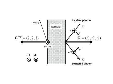
Figure 3: Schematic diagrams of the RXS geometry. The setting is adopted from Ref. Matsumura et al., 2009

In the following, we shall report the numerical results of the RXS spectra. First, we clarify the setting of our RXS calculation. A schematic aspect is found in Fig. 3, in which the scattering vector G and the photon polarization are depicted. Contrary to our definition of G, some literatures, including the experimental works we analyze in the following,Matsumura et al. (2009); Nakao et al. (2001) adopt the opposite sign, i.e., $\textbf{G}^{\textrm{exp}}=\textbf{k}-\textbf{k}^{\prime}$. To avoid a confusion, when we mention G in this section, we mean $\textbf{k}-\textbf{k}^{\prime}$, while the actual calculations are carried out by using $\textbf{k}^{\prime}-\textbf{k}$, because the formulae derived in our previous papers are the results of the latter definition.

IV.1 At $\textbf{G}=(\frac{3}{2}\frac{3}{2}\frac{1}{2})$ under $\textbf{H}//(\overline{1}10)$

IV.1.1 at the Ce $L_{3}$-edge

Figure 4: RXS spectra around the Ce $L_{3}$ edges at $\textbf{G}=(\frac{3}{2}\frac{3}{2}\frac{1}{2})$ with $\textbf{H}\parallel(\overline{1}10)$. Bold solid and bold broken lines represent $I_{\pi-\sigma^{\prime}}(\omega,+\textbf{H})$ and $I_{\pi-\sigma^{\prime}}(\omega,-\textbf{H})$, respectively. Inset: $I(\omega,\pm\textbf{H})$ around the $E$2 peak. Thin solid and thin broken lines represent $|\alpha_{1}^{(2)}(\omega)|^{2}[Z_{1}^{(2)}]^{2}$ and $|\alpha_{1}^{(2)}(\omega)Z_{1}^{(2)}+\alpha_{2}^{(2)}(\omega)Z_{2}^{(2)}|^{2}$, respectively.

Matsumura et al. carried out the RXS experiment under the applied magnetic field H along $(\overline{1}10)$ direction near Ce $L_{3}$ absorption edge at $\textbf{G}=(\frac{3}{2}\frac{3}{2}\frac{1}{2})$ in the $\pi$-incident polarization.Matsumura et al. (2009) They found the spectra showed strong enhancement of the intensity around the $E$1 and $E$2 regions. They also observed that the spectral shape underwent the significant change when the orientation of H was reversed. In particular, due to the cross term between the even rank and odd rank contributions, the spectra showed two-peak structure with peaks at the $E$1 and $E$2 positions when H was along $(\overline{1}10)$, while they showed single-peak structure with the $E$2 peak merged into the tail part of the $E$1 signal when H was along $(1\overline{1}0)$. We calculated the RXS spectra with the settings adjusted to those of Matsumura et al’s (Fig. 3). The results are shown in Fig. 4. The origins of the energy are set and fixed such that the $E$1 and $E$2 peaks become around 5724 eV and 5718 eV, respectively.

First, we concern the whole aspect of the spectral shapes. The calculated curves capture the above explained experimental feature well. We also confirm that the similar tendency is expected from the spectra in the $\sigma-\pi^{\prime}$ channel (not shown) with the intensity of the $E$1 peak being roughly a fourth of that in the $\pi-\sigma^{\prime}$ channel. Note that, the ratio of the intensity at the $E1$ peak to that at the $E$2 peak seems apparently quite different between the experiment and our result. For instance, for $+\textbf{H}$ ($|\textbf{H}|=2$ T), the ratio is about 2.45 in the experimentMatsumura et al. (2009) and about 9.66 in our calculation. A remedy for this discrepancy is absorption correction. The experimental ratio is enhanced to about 10.5 after the correction is properly carried out.com (c) So, our theoretical ratio gives fairly good values.

Next, we analyze the ingredients of the intensity around the $E$1 and $E$2 positions. To this aim, we define average intensity as

$$I_{\textrm{av}}(\omega)=\frac{I(\omega,+\textbf{H})+I(\omega,-\textbf{H})}{2}.$$ (22)

At the $E$1 peak, by using Eq. (10), the average intensity is approximated as

$$I_{\textrm{av}}(\omega)\simeq|\alpha_{1}^{(2)}(\omega)|^{2}[Z_{1}^{(2)}]^{2},$$ (23)

since another $E$1 contribution of $|\alpha_{1}^{(1)}(\omega)|^{2}[Z_{1}^{(1)}]^{2}$ is two orders of magnitude smaller than that of $|\alpha_{1}^{(2)}(\omega)|^{2}[Z_{1}^{(2)}]^{2}$. At the $E$2 peak, the situation is not so simple. As shown in the inset of Fig. 4, about half of the intensity around the $E$2 position is supplied by the tail part of the $E$1 contribution, $|\alpha_{1}^{(2)}(\omega)|^{2}[Z_{1}^{(2)}]^{2}$. Other than that, an even-rank profile of the $E$2 transition $\alpha_{2}^{(2)}(\omega)$ also has contribution by interfering with $\alpha_{1}^{(2)}(\omega)$ as illustrated by thin broken line. That is,

$$I_{\textrm{av}}(\omega)\simeq|\alpha_{1}^{(2)}(\omega)Z_{1}^{(2)}+\alpha_{2}^{(2)}(\omega)Z_{2}^{(2)}|^{2}.$$ (24)

Finally, we turn our attention to the difference spectrum $\Delta I(\omega)$ displayed in Fig. 5. The sign around $E$1 peak and that around $E$2 peak are opposite to each other, which is also in accordance with the experiment.Matsumura et al. (2009) Note that, as mentioned in Sec. I, although the $\Delta I(\omega)$ around the $E$1 region is not so prominent in Ref. Matsumura et al., 2009, its existence is assured by more careful measurement.com (a) The presence of $\Delta I(\omega)$ intensity at the $E$1 position, in itself, is ascribed to Eq. (14) of $\Delta I_{E1E1}$ $\propto\langle J_{z}\rangle\langle O_{\overline{1},1,0}\rangle$. It consists of the cross term between rank one and rank two contributions arose both from the $E$1 transition, which is missing within the fast collision approximation as stated before.

On the other hand, the origin of the intensity around the $E$2 peak is rather complicated. The whole shape is determined by $\Delta I_{E1E2}$, while both $\Delta I_{E1E1}$ and $\Delta I_{E2E2}$ have several quantitative contributions too. In the present setting, $Z_{2}^{(3)}$ is two orders of magnitude larger than $Z_{2}^{(1)}$ and the former is predominated by the contribution of $T_{xyz}$. Then, $\Delta I_{E1E2}(\omega)$ and $\Delta I_{E2E2}(\omega)$ are approximated as $2Z_{1}^{(2)}Z_{2}^{(3)}\textrm{Im}[\{\alpha_{2}^{(3)}(\omega)\}^{\star}\alpha_{1}^{(2)}(\omega)]$ and $2Z_{2}^{(3)}Z_{2}^{(2)}\textrm{Im}[\{\alpha_{2}^{(3)}(\omega)\}^{\star}\alpha_{2}^{(2)}(\omega)]$, respectively. Therefore, the entire spectral shape is well controlled by three energy profiles $\alpha_{1}^{(2)}(\omega)$, $\alpha_{2}^{(2)}(\omega)$, and $\alpha_{2}^{(3)}(\omega)$ carrying by the AFQ component of $O_{\overline{1},1,0}$ and AFO component of $T_{xyz}$.

Figure 5: Difference spectra around the Ce $L_{3}$ edges at $\textbf{G}=(\frac{3}{2}\frac{3}{2}\frac{1}{2})$ with $\textbf{H}\parallel(\overline{1}10)$ in the $\pi-\sigma^{\prime}$ channel. Bold solid line represents the total $\Delta I(\omega)$. Bold broken, bold dot-dashed, and thin solid lines are $\Delta I_{E1E1}(\omega),\Delta I_{E2E2}(\omega)$, and $\Delta I_{E1E2}(\omega)$, respectively.

Here, we end this subsection with the explanations concerning the robustness of the present results. Among several assumptions we have employed in the present work, the choice of the $5d$ DOS seems the most crucial one. The reason we have adopted the same DOS as used in our previous works is partly because to preserve the spherical symmetry in the intermediate states and partly to keep continuity of our research. Furthermore, we have confirmed that the characteristic features our data have shown are insensitive to the modification of the shape of the $5d$ DOS, fillingness of the $5d$ electron, and presence or absence of the DOS splitting between the $e_{g}$ and $t_{2g}$ states. For example, we have examined the semi-elliptic shape DOS and the uniform DOS. We also have changed the fillingness from 0.5 to 1.8 per Ce site and have introduced the DOS splitting between the $e_{g}$ and $t_{2g}$ states from $-3$ to $+3$ eV keeping the shape of the $5d$ DOS the same as that in Fig. 2. Although these modifications cause minor quantitative differences, the main features we stated in this section remain unchanged.

IV.1.2 at the Ce $L_{2}$-edge

Next, we also calculate the RXS spectra and the difference spectra expected from the AFQ phase in the vicinity of the Ce $L_{2}$ edge where the $E$1 and $E2$ transitions are observed around 6167 eV and 6160 eV, respectively. The results are shown in Fig. 6. The intensities are nearly the same as or slightly stronger than those at the $L_{3}$ edge (Fig. 4). We conclude that the RXS signal is experimentally detectable near the Ce $L_{2}$ absorption edge. Then, we concern the spectral shapes. One notable feature is the $E$2 process has no practical contribution. This shows a striking difference compared to the RXS spectra detected near the Ce $L_{2}$ edge in the antiferro-octupolar (AFO) phase of Ce_1-xLa_xB₆ where the signals from the $E$2 transition were distinctly observed.Mannix et al. (2005); Kusunose and Kuramoto (2005); Nagao and Igarashi (2006); Lovesey et al. (2007) The difference is attributed to that of the primary order parameter in these systems.

Figure 6: RXS spectra around the Ce $L_{2}$ edges at $\textbf{G}=(\frac{3}{2}\frac{3}{2}\frac{1}{2})$ with $\textbf{H}\parallel(\overline{1}10)$, respectively. (a) Solid and broken lines represent $I_{\pi\sigma^{\prime}}(\omega,+\textbf{H})$ and $I_{\pi\sigma^{\prime}}(\omega,-\textbf{H})$ in the $\pi-\sigma^{\prime}$ channels. Inset: $I(\omega,\pm\textbf{H})$ around the $E$2 peak. (b) $\Delta I_{\pi\sigma^{\prime}}(\omega)$ in the $\pi-\sigma^{\prime}$ channel.

IV.2 At $\textbf{G}=(\frac{1}{2}\frac{1}{2}\frac{1}{2})$ under $\textbf{H}//(11\overline{2})$

Nakao et al. detected the RXS signal of Ce $L_{3}$ edge from the AFQ phase.Nakao et al. (2001) However, their result practically showed no $E$2 contribution contrary to the present case reported by Matsumura et al., in which the peak intensity at the $E$2 transition has distinguishable contribution from that at the $E$1 transition.Matsumura et al. (2009) It is reasonable to interpret the difference is due to that of experimental conditions since the experiment by Nakao et al. was carried out at $\textbf{G}=(\frac{1}{2}\frac{1}{2}\frac{1}{2})$ under $\textbf{H}//(11\overline{2})$ and the polarization of the incident photon was $\sigma$ channel, all of which are different from the conditions chosen by Matsumura et al.

In our previous works, we analyzed Nakao et al.’s data and confirmed that the peak intensity at the $E$2 transition was negligible compared with the one at the $E$1 transition.Nagao and Igarashi (2001); Igarashi and Nagao (2002) In these treatments, we set the peak position of $E$2 transition about ten eV lower than that of $E$1 transition. It turns out that the interval is too wide, since it is about six eV as seen from Matsumura et al.’s data. If we set the $E$2 peak position at six eV lower than that of $E$1 transition, both intensities may experience interference even under the Nakao et al.’s experimental conditions. However, the calculated results (not shown), practically, have neither notable peak nor $\Delta I(\omega)$ intensities around the $E$2 position, which confirm our previous results survive after the shift of the $E$2 position. The absence of the distinct peak at the $E$2 position is merely the numerical reason. The tail part of the $E$1 contribution around the $E$2 position in Nakao et al.’s case is nearly twice larger than that in Matsumura et al.’s case. The former buries the $E$2 contribution, which is nearly the same in the latter case.

V Concluding Remarks

We have theoretically investigated the RXS spectra observed in the AFQ phase of CeB₆ in the vicinity of the Ce $L_{3}$ edge at $\textbf{G}=\left(\frac{3}{2},\frac{3}{2},\frac{1}{2}\right)$ under the applied field H along $\parallel(\overline{1},1,0)$ direction. The experimental data show small but clear contribution from the $E$2 process as well as that from the main $E$1 process. Also the interference between rank even and rank odd contributions from the $E$1 and/ or $E$2 signals are observed, which provides a great opportunity to obtain the information of the field-induced multipole orderings . To analyze the RXS spectra, we have employed the model on the basis of a localized electron picture, which is used in explaining several aspects of the RXS phenomena in CeB₆ and Ce_1-xLa_xB₆.Nagao and Igarashi (2001); Igarashi and Nagao (2002); Nagao and Igarashi (2003, 2006) The model is combined with the intermediate states including the intra-atomic Coulomb and the spin-orbit interactions within the appropriate electron configurations, so that the RXS signal is brought about by the Coulomb interaction.

The calculated spectra successfully capture the characteristic features the experimental data show: the ratio between the $E$1 and $E$2 intensities, the interference effect between the terms of rank even and odd when the direction of the magnetic field is reversed, and the signs of the difference spectrum $\Delta I(\omega)$ around the $E$1 and $E$2 regions.

When we focus on the detail of the spectra, the whole shape of the spectrum is roughly approximated by $I_{\textrm{av}}=|\alpha_{1}^{(2)}(\omega)Z_{1}^{(2)}+\alpha_{2}^{(2)}(\omega)Z_{2}^{(2)}|^{2}$, i.e., contributions from the AFQ order parameter are dominant. Even around the $E$2 region, about half of the intensity is supplied by the tail part of the $E$1 signal. On the other hand, the difference spectrum $\Delta I(\omega)$ is a direct consequence of the cross terms between the primary AFQ order and the magnetic-induced secondary order parameters with odd rank. A finite intensity of $\Delta I(\omega)$ around the $E$1 peak, $\Delta I_{E1E1}(\omega)$, is observed by both the experiment and our calculation. This term is absent within the fast collision approximation. The $\Delta I(\omega)$ around the $E$2 position consists of $\Delta I_{E1E2}(\omega)+\Delta I_{E2E2}(\omega)$. Comparing the $\Delta I(\omega)$ with the fitting curve based on the fast collision approximation constructed by two Lorentzian curves in Ref. 31, we see that both give relatively similar outlooks. However, this is a coincidence. Our analysis have showed the main ingredients of the entire spectrum are four profiles $\alpha_{2}^{(1)}(\omega)$, $\alpha_{2}^{(2)}(\omega)$, $\alpha_{1}^{(1)}(\omega)$, and $\alpha_{3}^{(2)}(\omega)$. We suggest that the difference of the spectral shape between our calculation and the outcome of the fast collision approximation may be observed when the orientation of the applied field is changed since the mixing ratios of four profiles are modified. A research toward this direction will be a future work.

We also have found that the RXS signal is strong enough to be detected experimentally at the $L_{2}$ edge, though the $E$2 peak is practically absent. We assert that the spectral analysis based on the microscopic calculation, which is beyond mere symmetrical consideration, is very useful to get deeper insights of the RXS phenomena.

As mentioned in the preceding section, most of our results are robust semi-quantitatively when several modifications are introduced into the $5d$ DOS. An exception is the fine structure of $\Delta I(\omega)$. Utilizing the better (and/or realistic) $5d$ DOS may improve the detail of $\Delta I(\omega)$. There is a suggestion that the $5d$ DOS of the $e_{g}$ and $t_{2g}$ states are splitting and have the different shapes derived by a electronic structure calculation.com (d) The splitting is expected at least in the high temperature region.Makita et al. (2008) We have checked, however, that such difference modifies little the overall shape of $I_{\textrm{av}}(\omega)$, while it affects in a subtle way that of $\Delta I(\omega)$. If the latter spectrum would be measured with more precision, the spectral shape can be used to infer the form of the $5d$ DOS.

A recent experimental report on magnetic spin resonance suggested that the AFQ-based model such as adopted in the present work met a difficulty in explaining its experimental data.Demishev et al. (2009) Even if a tiny amount of antiferromagnetic (AFM) moment is present, our results survive as long as the moment is small. A further test to our theory can be performed when the RXS signals are experimentally examined in the AFM phase.