First passage time distribution for a random walker on a random forcing energy landscape

Abstract

We present an analytical approximation scheme for the first passage time distribution on a finite interval of a random walker on a random forcing energy landscape. The approximation scheme captures the behavior of the distribution over all timescales in the problem. The results are carefully checked against numerical simulations.

I Introduction

The dynamics of a random walker on a one-dimensional random forcing (RF) energy landscapes has been a subject of much interest over the last three decades. Part of the interest is due to dynamics in quenched disordered systems. Examples are the dynamics of a random-field Ising model Bru84 ; Gri84 ; May84 ; Nat88 and the motion of dislocations in disordered crystals Hlr68 . More recently much interest has been due to many application in biophysical settings. It seems that in such systems random forcing energy landscapes are the rule and not the exception. In this context, the dynamics of random walkers on random forcing energy landscapes have found applications in the mechanical unzipping of DNA LN2000 ; DCBLNP2003 ; WLKDNP2005 , translocation of biomolecules through nanopores Mel2004 and the dynamics of molecular motors Harms1997 ; Kafri2004 ; Kafri2005 ; Hexner2009 . In many of these experiments the first passage time (FPT) distribution is directly measurable and in some, such as in the translocation of biomolecules through nanopores, it is the most direct measurement.

On a lattice the dynamics of the random walker is defined through the hopping rates between neighboring sites. We denote the hopping rate from site $i$ to site $i+1$ by $p_{i}$ and from site $i$ to site $i-1$ by $q_{i}$. To generate a RF energy landscape the sets of rates $\left\{p_{i}\right\}$ and $\left\{q_{i}\right\}$ are drawn randomly from distributions $p\left(p_{i}\right)$ and $q\left(q_{i}\right)$ respectively (both distributions are independent of $i$). It is convenient to introduce an energy difference variables $\left\{E_{i}\right\}$ such that $\frac{p_{i-1}}{q_{i}}=e^{-E_{i}}$ (measuring energies in units of $k_{B}T$). Thus each realization of the environment in the RF model can also be drawn as a set of i.i.d. random variables $\left\{q_{i}\right\}$ and $\left\{E_{i}\right\}$. Note that the energy landscape in this model is itself described by a biased random walk in energy space (see Fig. 1 for an illustration).

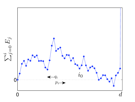
Figure 1: An illustration of a RF energy landscape. At site $d+1$ there is a reflecting boundary. Here $d=50$ and $\mu=0$. The energy difference between neighboring sites, $E_{i}$, is drawn from the Gaussian distribution.

It is well known Sin82 ; Der83a ; Kes75 ; Sol75 that the long-time and infinite lattice asymptotics of a random walker on such an energy landscape is rather rich. In particular, the dynamics are controlled by a parameter, $\mu=\left|\widetilde{\mu}\right|$, defined through the non-zero solution of the equation Der83a ; Kes75 ; Der82b

$$\left\langle\left(\frac{p_{i}}{q_{i+1}}\right)^{\widetilde{\mu}}\right\rangle=1,$$ (1)

where the angular brackets represent an average of realizations of disorder or, equivalently, over the distributions of $\left\{p_{i}\right\}$ and $\left\{q_{i}\right\}$. For $\mu>2$ the behavior is similar to that of a biased random walker on a flat energy landscape. Namely, for large times the mean position $\left\langle\overline{x}\right\rangle$ and its variance $\left\langle\overline{\left(x-\overline{x}\right)^{2}}\right\rangle$ both grow linearly in time (here the overline denotes an average over histories of the system starting from the same initial position). In this regime both quantities are self averaging. When $0<\mu<2$ the behavior is anomalous. For $1<\mu<2$ the mean displacement is self averaging and $\overline{x}\sim\left\langle\overline{x}\right\rangle\sim t$. The diffusion, however, behaves as $\overline{\left(x-\overline{x}\right)^{2}}\sim t^{2/\mu}$ while its average over realizations of disorder behaves as $\left\langle\overline{\left(x-\overline{x}\right)^{2}}\right\rangle\sim t^{3-\mu}$. For $0<\mu<1$ both the drift and the diffusion are anomalous. Asymptotically the velocity, defined through $\underset{t\rightarrow\infty}{\lim}\left\langle\overline{x}\right\rangle/t$, vanishes. Specifically, the drift behaves as $\overline{x}\sim\left\langle\overline{x}\right\rangle\sim t^{\mu}$ (note that although $\overline{x}\$and $\left\langle\overline{x}\right\rangle$ have the same scaling $\overline{x}$ is not a self-averaging quantity BG90 ). In addition $\overline{\left(x-\overline{x}\right)^{2}}\sim t^{2/\mu}$ and its average over the realizations of disorder behaves as $\left\langle\overline{\left(x-\overline{x}\right)^{2}}\right\rangle\sim t^{3-\mu}$. Finally, when $\mu=0$ (commonly referred to as Sinai diffusion) $\overline{x}\sim\ln^{2}t$, $\left\langle\overline{x}\right\rangle=0$, $\overline{x^{2}}\sim\left\langle\overline{x^{2}}\right\rangle\sim\ln^{4}t$ Sin82 and $\overline{\left(x-\overline{x}\right)^{2}}\sim\left\langle\overline{\left(x-\overline{x}\right)^{2}}\right\rangle\sim t^{0}$ Golosov84 .

In this paper we provide an approximation for the FPT distribution of a random walker on a RF energy landscapes in a finite interval. Namely, we are interested in the disorder averaged FPT probability density from site $i_{0}\geq 0$ to the origin (site $0$), $F\left(t\right)=\left\langle F_{i_{0}\rightarrow 0}\left(t|\left\{p_{i},q_{i}\right\}\right)\right\rangle$ with reflecting boundary conditions at lattice site $d+1$ with $d\geq i_{0}$, so that $p_{d}=0$ or $E_{d+1}=\infty$ (see Fig. 1). The results are summarized in Sec. VI. Note that this rather rich behavior makes it impossible to write the averaged propagator of the process as a scale invariant function, except in the Sinai’s case $\mu=0$. Therefore, the techniques developed in Vut1 ; Vut2 to calculate the distribution of FPTs for scale invariant processes are not directly applicable. Our results are compared with numerical calculations and shown to agree very well. To obtain the approximation we present a ”random tilt” (RT) model, similar in spirit, to that used in Osh09 . The parameters which define the RT model are given in terms of the parameters of a random walker on a RF energy landscape (for simplicity we assume a walker on a lattice) with no fitting parameters. This model naturally exhibits all of the regimes exhibited by other RF models after a proper disorder average. Specifically, within the model we obtain an exact result for the Laplace transform

$$\widetilde{F}\left(s\right)=\int_{0}^{\infty}F\left(t\right)e^{-st}dt$$ (2)

of the FPT between two given points with specified boundary condition. The Laplace transform can be easily inverted numerically.

The paper is organized as follows: in Sec. II we present a brief review of relevant known results for a random walker on a RF energy landscape. In Sec. III we present and solve the RT model. In Secs. V.2 and V.1 we determine the parameters of the RT model which are used to approximate the FPT probability density of the RF model. In Sec. V.3 we compare the approximation to numerical results.

II Review of some known results for a random walker on a RF energy landscape

While the exact full FPT distribution, $F\left(t\right)$, for which we provide an approximation, is not known, several related results are known. Specifically, the mean FPT, defined through $\left\langle\overline{t}\right\rangle=\int_{0}^{\infty}tF\left(t\right)dt$, can be obtained using the expression for a given realization of disorder (namely, a given set of $\left\{E_{i}\right\}$ and $\left\{q_{i}\right\}$) Mur89

$$\overline{t}=\underset{i=1}{\overset{i_{0}}{{\displaystyle\sum}}}\left(\frac{1}{q_{d}}\underset{j=i_{0}}{\overset{d-1}{{\displaystyle\prod}}}\frac{p_{j}}{q_{j}}+\underset{k=1}{\overset{d-1}{{\displaystyle\sum}}}\frac{1}{q_{k}}\underset{j=i}{\overset{k-1}{{\displaystyle\prod}}}\frac{p_{j}}{q_{j}}\right),$$ (3)

where, as stated above, $\frac{p_{i-1}}{q_{i}}=e^{-E_{i}}$. Therefore, the disorder average of $\overline{t}$ is

$$\left\langle\overline{t}\right\rangle=\left\langle\frac{1}{q_{i}}\right\rangle\frac{\left\langle e^{-E_{i}}\right\rangle^{d+1}-\left\langle e^{-E_{i}}\right\rangle^{d-i_{0}+1}}{\left(\left\langle e^{-E_{i}}\right\rangle-1\right)^{2}}-\left\langle\frac{1}{q_{i}}\right\rangle\frac{i_{0}}{\left\langle e^{-E_{i}}\right\rangle-1}.$$ (4)

Note that this quantity may be very different from the typical FPT, defined through $\exp\left\langle\ln\overline{t}\right\rangle$ (see for example Dou89b for a discussion of the Sinai’s case $\mu=0$). From Eq. (3) one may see that in the large $d$ limit the leading order of $\left\langle\ln\overline{t}\right\rangle$ is $\underset{j=1}{\overset{d}{\sum}}\ln\frac{p_{j}}{q_{j}}=-Ed$, where $E=\left\langle E_{i}\right\rangle$ is the average tilt of the RF energy landscape. Therefore, the typical FPT scales as

$$\exp\left\langle\ln\overline{t}\right\rangle\sim e^{-Ed},$$ (5)

increasing exponentially with $d$ for $E<0$ and remaining constant for $E>0$.

In the limit $d\rightarrow\infty$ the FPT probability density for $E<0$ is not normalizable since the probability to never pass $i=0$ is positive. For the $E>0$ (and $d\rightarrow\infty$) case it is known BG90 ; Dou99 that the mean FPT distribution density scales as $\overline{t}^{-(1+\mu)}$ for large $\overline{t}$. This implies that the value of $\mu$ may be evaluated by finding the largest converging moment of the mean FPT for $d\rightarrow\infty$. Equivalently, $\mu$ is given by the smallest moment that diverges

$$\mu=\inf\left\{m:\left\langle\overline{t}^{m}\right\rangle=\infty\right\}.$$ (6)

To obtain an approximation for the full FPT distribution, in the next section we introduce and solve a RT model. The parameters of the RT model are set by the known properties of the RF model.

III The random tilt model

Recently Oshanin and Redner Osh09 used an optimal fluctuation method Lif88 to study the splitting probability, $P$, of a random walker on a random forcing energy landscape. The splitting probability is defined as the probability to reach site $i=d$ before hitting site $i=0$, starting from site $i=i_{0}$. Within this approach one replaces each specific realization of the random forcing energy landscape by its average slope, $U$, which is specified by the energy difference between the origin and the last, $i=d$, site divided by the total number of the sites (see Fig. 2). The central limit theorem implies that the probability density of the average energy tilt is Gaussian:

$$\Pr\left(U\right)=\frac{e^{-d\frac{\left(U-E\right)^{2}}{2\sigma^{2}}}}{\sqrt{2\pi\frac{\sigma^{2}}{d}}},$$ (7)

where $E$, as stated before, is the average energy difference between two subsequent sites

$$E=\left\langle E_{i}\right\rangle=\left\langle\ln\frac{q_{i}}{p_{i-1}}\right\rangle$$ (8)

and $\sigma^{2}$ is the variance of the energy difference between two subsequent sites

$$\sigma^{2}=\left\langle E_{i}^{2}\right\rangle-\left\langle E_{i}\right\rangle^{2}=\left\langle\ln^{2}\frac{q_{i}}{p_{i-1}}\right\rangle-\left\langle\ln\frac{q_{i}}{p_{i-1}}\right\rangle^{2}.$$ (9)

Using the fact that on a constant energy tilt, $U$, the splitting probability is given by $\frac{1-e^{Ui_{0}}}{1-e^{Ud}}$ Fel66 the average splitting probability can be well approximated by Osh09

$$P\simeq\int_{-\infty}^{\infty}\frac{e^{-d\frac{\left(U-E\right)^{2}}{2\sigma^{2}}}}{\sqrt{2\pi\frac{\sigma^{2}}{d}}}\frac{1-e^{Ui_{0}}}{1-e^{Ud}}dU.$$ (10)

Figure 2: On this schematic plot we demonstrate the approach described in Osh09 where each specific realization of the disordered is replaced by constant energy slope.

Inspired by this approach we introduce a random tilt (RT) model. Within the model the energy landscape of each realization is flat while its tilt is a random variable. Namely, defining hopping rates to the right and left by $u$ and $v$ respectively, with $\frac{u}{v}=e^{-\varepsilon}$, we take $\varepsilon$ to be a random variable with a Gaussian probability density

$$\Pr\left(\varepsilon\right)=\frac{1}{\sqrt{2\pi\sigma_{\varepsilon}^{2}/d}}e^{-d\frac{\left(\varepsilon-\left\langle\varepsilon\right\rangle\right)^{2}}{2\sigma_{\varepsilon}^{2}}}$$ (11)

with a mean $\left\langle\varepsilon\right\rangle$ and a variance $\sigma_{\varepsilon}^{2}$. Here $d$, as before, is the size of the system. As we show below by fixing $\left\langle\varepsilon\right\rangle$, $\sigma_{\varepsilon}$ and an overall time we can approximate very well the first passage behavior of a random walker on a RF energy landscape in the limit $d\rightarrow\infty$ and large $t$. We refer to this as the universal regime. In this paper, however, we are interested in an approximation over any time scale when $d$ is finite. In this case the small $t$ and large $t$ behaviors are not universal. As we show a very good approximation can be achieved by taking the value of $v$ as a random variable with its own distribution $\Pr\left(v\right)$. In Secs. V.1 and V.2 we show that, in order to approximate the FPT probability density of the RF model, the simplest choice one can make is

$$\Pr\left(v\right)=\pi_{1}\delta\left(v-v_{1}\right)+\pi_{2}\delta\left(v-v_{2}\right)+\left(1-\pi_{1}-\pi_{2}\right)\delta\left(v-v_{3}\right).$$ (12)

The values of $\left\langle\varepsilon\right\rangle$, $\sigma_{\varepsilon}$, $v_{1}$, $v_{2}$, $v_{3}$, $\pi_{1}$ and $\pi_{2}$ are set by known properties of the RF model (with no fitting parameters). As stated above, the results are summarized at the end of the paper. Note that to approximate only part of the FPT distribution a simpler choice of $\Pr\left(v\right)$ can be made. For example, if one is not interested in the short time behavior one can chose $\Pr\left(v\right)=\delta\left(v-v_{0}\right)$ where $v_{0}$ is specified in what follows (see Eq. (33) below). If one is not interested in the long time behavior but wants to capture the short time behavior one can chose $\Pr\left(v\right)=\delta\left(v-\left\langle q\right\rangle\right)$ (see Eq. (37) below).

IV The properties of the RT model

To approximate the FPT distribution on a RF energy landscape we evaluate the splitting probability of the RT model, $P_{RT}$, the analog of the exponent $\mu$ of the RT model, denoted by $\mu_{RT}$ and the average FPT, denoted by $\left\langle\overline{t}\right\rangle_{RT}$. In addition we also calculate the Laplace transform of the FPT probability density of the RT model, $\widetilde{F}_{RT}\left(s\right)$.

The splitting probability of the RT model can be easily obtained, similar to Eq. (10), and is given by

$$P_{RT}=\int_{-\infty}^{\infty}\frac{e^{-d\frac{\left(\varepsilon-\left\langle\varepsilon\right\rangle\right)^{2}}{2\sigma_{\varepsilon}^{2}}}}{\sqrt{2\pi\frac{\sigma_{\varepsilon}^{2}}{d}}}\frac{1-e^{\varepsilon i_{0}}}{1-e^{\varepsilon d}}d\varepsilon.$$ (13)

Note that Eq. (13) is exact for the RT model.

First we demonstrate that an analog of $\mu$, denoted by $\mu_{RT}$, exists for the RT model when $d\rightarrow\infty$. This shows that indeed the model can reproduce a qualitative first passage behavior similar to a random walker on a RF energy landscape. To do this we calculate the scaling behavior of the moments of the average FPT, $\overline{t}_{\varepsilon}$. For a given realization of $\varepsilon$ (the equivalent of a random realization of the RF energy landscape) this scales as

$$\overline{t}_{\varepsilon}=\frac{1}{v}\frac{\left(\frac{u}{v}\right)^{d}-1}{\frac{u}{v}-1}\sim\left\{\begin{array}[c]{cc}e^{-\varepsilon d}&\varepsilon<0\\ \frac{1}{v}\frac{1}{1-e^{-\varepsilon}}&\varepsilon>0\end{array}\right..$$ (14)

Recalling that the probability density of $\varepsilon$ is Gaussian

$$\Pr\left(\varepsilon\right)\sim e^{-d\frac{\left(\varepsilon-\left\langle\varepsilon\right\rangle\right)^{2}}{2\sigma_{\varepsilon}^{2}}}\;,$$ (15)

and in analogy with the RF model (see Eq. (6)), $\mu_{RT}$ is given by

$$\mu_{RT}=\inf\left\{m:\left\langle\overline{t_{\varepsilon}}^{m}\right\rangle=\infty\right\},$$ (16)

where now the angular brackets denote an average over $\varepsilon$ values. In the $d\rightarrow\infty$ limit, when $\left\langle\overline{t_{\varepsilon}}^{m}\right\rangle=\infty$, the average of the $m$’th moment is controlled by the contributions where $\varepsilon<0$ so that

$$\left\langle\overline{t}_{\varepsilon}^{m}\right\rangle\sim e^{\left(-m\left\langle\varepsilon\right\rangle+m^{2}\frac{\sigma_{\varepsilon}^{2}}{2}\right)d}.$$ (17)

We, therefore, obtains

$$\mu_{RT}=\left|\frac{2\left\langle\varepsilon\right\rangle}{\sigma_{\varepsilon}^{2}}\right|.$$ (18)

Thus, as stated above, an analog of $\mu$ exists within the RT model after averaging over realizations of disorder. It, of course, does not exist for each realization of the model. Note that this expression is identical to that obtained for a full random forcing model where the random force is drawn from a Gaussian distribution with a mean $\langle\varepsilon\rangle$ and variance $\sigma_{\varepsilon}^{2}$ BG90 . Furthermore, Eq. (14) implies that the scaling behavior of the typical FPT is given by

$$\exp\left\langle\ln\overline{t}\right\rangle_{RT}\sim e^{-\left\langle\varepsilon\right\rangle d},$$ (19)

increasing exponentially with $d$ for $\left\langle\varepsilon\right\rangle<0$ and remaining constant when $\left\langle\varepsilon\right\rangle>0$.

Next we consider the mean FPT of the RT model (averaged over realizations of the tilt of the landscape) to the origin from site $i_{0}$. For a given energy tilt, $\varepsilon$, and a given left hopping rate, $v$, the thermal averaged FPT may be obtained using Eq. (3) with the substitutions $\left\langle\frac{1}{q_{i}}\right\rangle=\frac{1}{v}$ and $\left\langle e^{-E_{i}}\right\rangle=e^{-\varepsilon}$. Averaging over $\varepsilon$ and $v$ one obtains

$$\left\langle\overline{t}\right\rangle_{RT}=\left\langle\frac{1}{v}\right\rangle I$$ (20)

where

$$I=\int_{-\infty}^{\infty}\left[\frac{e^{-\varepsilon\left(d+1\right)}-e^{-\varepsilon\left(d-i_{0}+1\right)}}{\left(e^{-\varepsilon}-1\right)^{2}}-\frac{i_{0}}{e^{-\varepsilon}-1}\right]\frac{e^{-d\frac{\left(\varepsilon-\left\langle\varepsilon\right\rangle\right)^{2}}{2\sigma_{\varepsilon}^{2}}}}{\sqrt{2\pi\frac{\sigma_{\varepsilon}^{2}}{d}}}d\varepsilon$$ (21)

and

$$\left\langle\frac{1}{v}\right\rangle=\int_{0}^{\infty}\frac{1}{v}\Pr\left(v\right)dv.$$ (22)

The Laplace transform of the FPT probability density can also be obtained exactly and is given by

$$\widetilde{F}_{RT}\left(s\right)=\int\int\Pr\left(\varepsilon\right)\Pr\left(v\right)\Phi\left(\frac{s}{v},\varepsilon\right)d\varepsilon dv,$$ (23)

where $\Phi\left(\frac{s}{v},\varepsilon\right)$ is the FPT probability density on a flat energy landscape with a tilt $\varepsilon$ and a left hopping rate $v$. Using standard FPT results Fel66 one has

$$\Phi\left(\frac{s}{v},\varepsilon\right)=\frac{\lambda_{2}^{i_{0}}\left(\frac{s}{v},\varepsilon\right)}{2^{i_{0}}}\frac{1-\left(\frac{\lambda_{2}\left(\frac{s}{v},\varepsilon\right)}{\lambda_{1}\left(\frac{s}{v},\varepsilon\right)}\right)^{d-i_{0}-1}\frac{\left(\frac{s}{v}+1\right)\lambda_{2}\left(\frac{s}{v},\varepsilon\right)-2}{\left(\frac{s}{v}+1\right)\lambda_{1}\left(\frac{s}{v},\varepsilon\right)-2}}{1-\left(\frac{\lambda_{2}\left(\frac{s}{v},\varepsilon\right)}{\lambda_{1}\left(\frac{s}{v},\varepsilon\right)}\right)^{d-1}\frac{\left(\frac{s}{v}+1\right)\lambda_{2}\left(\frac{s}{v},\varepsilon\right)-2}{\left(\frac{s}{v}+1\right)\lambda_{1}\left(\frac{s}{v},\varepsilon\right)-2}}$$ (24)

with

$$\lambda_{1,2}\left(\frac{s}{v},\varepsilon\right)=1+\left(1+\frac{s}{v}\right)e^{\varepsilon}\pm\sqrt{1+2e^{\varepsilon}\left(\frac{s}{v}-1\right)+e^{2\varepsilon}\left(\frac{s}{v}+1\right)^{2}}.$$ (25)

Next we use these results to approximate the FPT distribution in the RF model.

V Approximating the FPT distribution of the RF model

To use the results to approximate the FPT probability density of the RF model here we set the parameters $\left\langle\varepsilon\right\rangle$ and $\sigma_{\varepsilon}^{2}$ and the probability distribution $\Pr\left(v\right)$, such that $\widetilde{F}_{RT}\left(s\right)$ yields a good approximation to $\widetilde{F}\left(s\right)$. Namely, we work with the Laplace transform. The matching is done so the distributions agree in different ranges of $s$ and can be done by matching between known quantities of both the RT and the RF models. We first determine the parameters $\left\langle\varepsilon\right\rangle$ and $\sigma_{\varepsilon}$.

V.1 Determining $\left\langle\varepsilon\right\rangle$ and $\sigma_{\varepsilon}$

Here we find expressions for $\left\langle\varepsilon\right\rangle$ and $\sigma_{\varepsilon}$ by matching the scaling properties of the FPT probability densities. The value of $\left\langle\varepsilon\right\rangle$ may be found by matching the scaling behavior of the typical FPT of the two models in the large $d$ limit. We showed above (see Eq. (5)) that in the RF model the typical FPT grows as $e^{-Ed}$ for $E<0$ and remains constant while $E>0$ (see Eq. (14)). The same is true (see Eq. (19)) for the RT model when $E$ is replaced by $\left\langle\varepsilon\right\rangle$. Thus to match the scaling behavior of the typical FPT in both models we set

$$\left\langle\varepsilon\right\rangle=E.$$ (26)

The scaling properties in the intermediate $s$ regime for a finite value of $d$ can be expected to behave identically to the small $s$ behavior of the $d\rightarrow\infty$ limit. Since the scaling behavior is different for negative and positive average tilts we separate our discussion to two cases.

V.1.1 The case $E<0$

In this case the splitting probability, $P$, remains finite in the $d\rightarrow\infty$ limit. Thus, the small $s$ behavior of the FPT probability density in the $d\rightarrow\infty$ limit is $1-P+O\left(s\right)$. To match the intermediate $s$ behavior of FPT probability density of RF and RT models we match the splitting probabilities (i.e. the leading, $O\left(s^{0}\right)$, order of the FPT probability densities) of these two models.

Comparing (10) with (13) and using Eq. (26) yields

$$\sigma_{\varepsilon}=\sigma.$$ (27)

Note that both the average tilt and the variance in the RF and RT models are equal in this regime.

V.1.2 The case $E>0$

As studied in Sec. I, in this case the mean FPT distribution for $d\rightarrow\infty$ in the small $s$ region scales as $1-O\left(s^{\mu}\right)$ for $\mu<1$ (or, equivalently in time as $\overline{t}^{-\left(1+\mu\right)}$). Therefore, we first match $\mu_{RT}$ of the RT model with $\mu$ of the RF model. Namely, we set $\mu_{RT}=\mu$. Using Eq. (18) this yields

$$\frac{2\left\langle\varepsilon\right\rangle}{\sigma_{\varepsilon}^{2}}=\mu.$$ (28)

Solving Eqs. (26) and (28) we get

$$\sigma_{\varepsilon}=\sqrt{\frac{2E}{\mu}}.$$ (29)

Note when the distribution of $E_{i}$ is Gaussian equations (27) and (29) become identical. Namely, both the average tile and the variance of the RF and RT models are equivalent. When the distribution is not Gaussian the average tilt is the same in both models but the variances can be different. In this regime it is important to match the precise value of $\mu$ rather than the splitting probability as in the $E<0$ case.

V.2 Determination of $\Pr\left(v\right)$

In this section we choose the distribution $\Pr\left(v\right)$ by matching the FPT probability density of the RT model to that of the original RF system in the small and large $s$ limits. We show that for each limit one may choose $v$ to be a constant. However, this constant depends on the limit. Thus, to match the full $s$ behavior $v$ cannot be a constant and, as we show below, the simplest choice for $\Pr\left(v\right)$ is

$$\Pr\left(v\right)=\pi_{1}\delta\left(v-v_{1}\right)+\pi_{2}\delta\left(v-v_{2}\right)+\left(1-\pi_{1}-\pi_{2}\right)\delta\left(v-v_{3}\right)$$ (30)

with $v_{1,2,3}$ are set according to relevant time scales in the problem and $\pi_{1,2}$ are determined by the matching procedure, described below.

V.2.1 The small $s$ approximation

The $s\rightarrow 0$ behavior of the FPT probability densities of the RF and the RT models is

$$\widetilde{F}\left(s\rightarrow 0\right)=1-\left\langle\overline{t}\right\rangle s$$ (31)

and

$$\widetilde{F}_{RT}\left(s\rightarrow 0\right)=1-\left\langle\overline{t}\right\rangle_{RT}s,$$ (32)

respectively. Therefore, to match $\widetilde{F}\left(s\rightarrow 0\right)$ and $\widetilde{F}_{RT}\left(s\rightarrow 0\right)$ one has to match the mean FPTs of both models. Demanding $\left\langle\overline{t}\right\rangle_{RT}=\left\langle\overline{t}\right\rangle$ and using Eq. (20) one has

$$\left\langle\frac{1}{v}\right\rangle=\frac{\left\langle\overline{t}\right\rangle}{I}$$ (33)

where $I$ is defined in Eq. (21) and $\left\langle\overline{t}\right\rangle$ is given by Eq. (4).

Below we use this fact to match the behavior of the FPT distribution of the RF model over the whole $s$ range. Note however, that if one is not interested in the short time behavior the procedure is simplified. One can then choose $\Pr\left(v\right)=\delta\left(v-v_{1}\right)$ where $v_{1}=\frac{I}{\left\langle\overline{t}\right\rangle}$. Then, using Eq. (23), the Laplace transform of the FPT probability density is given by

$$\widetilde{F}_{RT}\left(s\right)=\int_{-\infty}^{\infty}\frac{e^{-d\frac{\left(\varepsilon-\left\langle\varepsilon\right\rangle\right)^{2}}{2\sigma_{\varepsilon}^{2}}}}{\sqrt{2\pi\frac{\sigma_{\varepsilon}^{2}}{d}}}\Phi\left(\frac{s}{v_{1}},\varepsilon\right)d\varepsilon.$$ (34)

V.2.2 The large $s$ approximation

The large $s$ limit corresponds to the small $t$ limit. This regime of the FPT distribution is controlled by walks which hop only to the left before reaching the origin. Therefore, in the $s\rightarrow\infty$ limit the behavior of the FPT probability densities of the RF and the RT models is

$$\widetilde{F}\left(s\rightarrow\infty\right)=\left\langle q\right\rangle^{i_{0}}$$ (35)

and

$$\widetilde{F}_{RT}\left(s\rightarrow\infty\right)=\left\langle v^{i_{0}}\right\rangle,$$ (36)

respectively. Thus, to match the large $s$ behavior of $\widetilde{F}_{RT}\left(s\right)$ and $\widetilde{F}\left(s\right)$ we demand

$$\left\langle v^{i_{0}}\right\rangle=\left\langle q\right\rangle^{i_{0}}.$$ (37)

Next we match the behaviors in the RT and RF models over the whole range of $s$. However, we comment that if one is not interested in the approximate FPT distribution in the long time limit one can choose $\Pr\left(v\right)=\delta\left(v-v_{2}\right)$ where $v_{2}=\left\langle q\right\rangle$. Then, using Eq. (23), the Laplace transform of the FPT probability density is given by

$$\widetilde{F}_{RT}\left(s\right)=\int_{-\infty}^{\infty}\frac{e^{-d\frac{\left(\varepsilon-\left\langle\varepsilon\right\rangle\right)^{2}}{2\sigma_{\varepsilon}^{2}}}}{\sqrt{2\pi\frac{\sigma_{\varepsilon}^{2}}{d}}}\Phi\left(\frac{s}{v_{2}},\varepsilon\right)d\varepsilon.$$ (38)

V.2.3 An approximation for the whole $s$ range

To match both the small and large $s$ limit one should supply $\Pr\left(v\right)$ such that Eqs. (33) and (37) are satisfied. However, these equations do not determine $\Pr\left(v\right)$ uniquely and there is a lot of freedom. As stated above, the simplest choice that satisfies these equations is

$$\Pr\left(v\right)=\pi_{1}\delta\left(v-v_{1}\right)+\pi_{2}\delta\left(v-v_{2}\right)+\left(1-\pi_{1}-\pi_{2}\right)\delta\left(v-v_{3}\right).$$ (39)

However, since one has to satisfy only two equations ((33) and (37)) there is still a lot of freedom with five free parameters. Therefore, first we set $v_{1,2,3}$ such that they represent relevant time scales in the problem. Eq. (33) suggests

$$\frac{1}{v_{1}}=\frac{\left\langle\overline{t}\right\rangle}{I},$$ (40)

while Eq. (37) suggests

$$v_{2}=\left\langle q\right\rangle.$$ (41)

The third time scale is chosen to represent the average time of a hop to the left

$$v_{3}=\left\langle\frac{1}{q}\right\rangle^{-1}.$$ (42)

Given these three quantities, $v_{1,2,3}$, Eqs. (33) and (37) give

$$\pi_{1}v_{1}^{i_{0}}+\pi_{2}v_{2}^{i_{0}}+\left(1-\pi_{1}-\pi_{2}\right)v_{3}^{i_{0}}=\left\langle\,q\right\rangle^{i_{0}}$$ (43)

and

$$\frac{\pi_{1}}{v_{1}}+\frac{\pi_{2}}{v_{2}}+\frac{1-\pi_{1}-\pi_{2}}{v_{3}}=\frac{\left\langle\overline{t}\right\rangle}{I}.$$ (44)

The solution for $\pi_{1,2}$ is

$$\pi_{1}=\frac{v_{1}\left\langle\overline{t}\right\rangle}{I}\frac{v_{2}v_{3}\left(v_{2}^{i_{0}}-v_{3}^{i_{0}}\right)+\frac{I\left\langle q\right\rangle^{i_{0}}}{\left\langle\overline{t}\right\rangle}\left(v_{2}-v_{3}\right)+\frac{I}{\left\langle\overline{t}\right\rangle}\left(v_{3}^{i_{0}+1}-v_{2}^{i_{0}+1}\right)}{v_{2}v_{3}\left(v_{2}^{i_{0}}-v_{3}^{i_{0}}\right)+v_{1}^{i_{0}+1}\left(v_{2}-v_{3}\right)+v_{1}\left(v_{3}^{i_{0}+1}-v_{2}^{i_{0}+1}\right)}$$ (45)

and

$$\pi_{2}=-\frac{v_{2}\left\langle\overline{t}\right\rangle}{I}\frac{v_{1}v_{3}\left(v_{1}^{i_{0}}-v_{3}^{i_{0}}\right)+\frac{I\left\langle q\right\rangle^{i_{0}}}{\left\langle\overline{t}\right\rangle}\left(v_{1}-v_{3}\right)+\frac{I}{\left\langle\overline{t}\right\rangle}\left(v_{3}^{i_{0}+1}-v_{1}^{i_{0}+1}\right)}{v_{2}v_{3}\left(v_{2}^{i_{0}}-v_{3}^{i_{0}}\right)+v_{1}^{i_{0}+1}\left(v_{2}-v_{3}\right)+v_{1}\left(v_{3}^{i_{0}+1}-v_{2}^{i_{0}+1}\right)}.$$ (46)

Using these quantities, the probability density (39) for $v$ and Eq. (23), the Laplace transform of the FPT probability density is given by

$$\widetilde{F}_{RT}\left(s\right)=\int_{-\infty}^{\infty}\frac{e^{-d\frac{\left(\varepsilon-\left\langle\varepsilon\right\rangle\right)^{2}}{2\sigma_{\varepsilon}^{2}}}}{\sqrt{2\pi\frac{\sigma_{\varepsilon}^{2}}{d}}}\left[\pi_{1}\Phi\left(\frac{s}{v_{1}},\varepsilon\right)+\pi_{2}\Phi\left(\frac{s}{v_{2}},\varepsilon\right)+\left(1-\pi_{2}-\pi_{3}\right)\Phi\left(\frac{s}{v_{3}},\varepsilon\right)\right]d\varepsilon.$$ (47)

In the next section we compare the obtained result to the numerical simulation. This expression with the above chosen values of parameters is the main result of our paper. Note that while quite a few parameters have to be set there are no free fitting parameters. As we show the agreement is very good.

V.3 FPT probability density and comparison to numerical result

In this section we compare between Eq. (47) and numerical simulations. Namely we compare the Laplace transform of the FPT probability, density, $\widetilde{F}_{RT}\left(s\right)$, and the survival probability

$$F_{S}\left(t\right)=1-\int_{0}^{t}F\left(t^{\prime}\right)dt^{\prime}$$ (48)

of the RF and RT models. We checked the results for RF models with both Bernoulli and Gaussian disorders.

For the RF system with Bernoulli disorder the energy difference on each site, $E_{i}$, is drawn from the distribution:

$$\Pr\left(E_{i}\right)=\left\{\begin{array}[c]{cc}r&E_{i}=\varepsilon_{1}\\ 1-r&E_{i}=\varepsilon_{2}\end{array}\right..$$ (49)

On Figs. 3,4,5 one may see the comparison between Eq. (47) and the numerical calculation in different parameter ranges. As can be seen the agreement is very satisfying.

For a RF model with a Gaussian disorder the energy difference between sites, $E_{i}$, is drawn from a normal distribution with a mean $E$ and a variance $\sigma^{2}$:

$$\Pr\left(E_{i}\right)=\frac{e^{-d\frac{\left(E_{i}-E\right)^{2}}{2\sigma^{2}}}}{\sqrt{2\pi\frac{\sigma^{2}}{d}}}.$$ (50)

On Figs. 6,7,8 we show a comparison between Eq. (47) and numerical calculation in different parameter ranges. Again, the results of the approximation are very good.

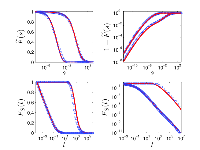
Figure 3: In this graph a comparison between the analytic approximation (47) and the numerical results for a Bernoulli disorder is shown in Laplace (top) and time (bottom) spaces. The parameters for these plots are: $r=0.5$, $\varepsilon_{1}=-0.4$, $\varepsilon_{2}=0.4$ and $d=100$, such that $\mu=0$. Circles represent the choice $i_{0}=1$ while squares represent the choice $i_{0}=50$ cases on both, left and right, figures. The red lines are analytic approximations based on Eq. (47).

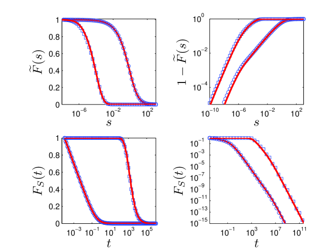
Figure 4: In this graph a comparison between the analytic approximation (47) and the numerical results for a Bernoulli disorder is shown in Laplace (top) and time (bottom) spaces. The parameters for these plots are: $r=0.49$, $\varepsilon_{1}=-0.1$, $\varepsilon_{2}=0.1$ and $d=550$, such that $\mu=0.4$. Circles represent the choice $i_{0}=1$ while squares represent the choice $i_{0}=100$ cases on both, left and right, figures. The red lines are analytic approximations based on Eq. (47).

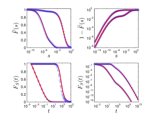
Figure 5: In this graph a comparison between the analytic approximation (47) and the numerical results for a Bernoulli disorder is shown in Laplace (top) and time (bottom) spaces. The parameters for these plots are: $r=0.58$, $\varepsilon_{1}=-0.3$, $\varepsilon_{2}=0.3$ and $d=150$, such that $\mu=-1.08$. Circles represent the choice $i_{0}=1$ while squares represent the choice $i_{0}=50$ cases on both, left and right, figures. The red lines are analytic approximations based on Eq. (47).

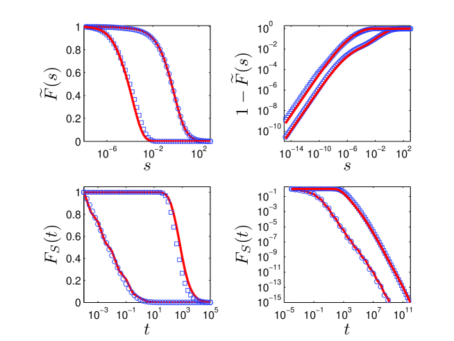
Figure 6: In this graph a comparison between the analytic approximation (47) and the numerical results for a Gaussian disorder is shown in Laplace (top) and time (bottom) spaces. The parameters for these plots are: $E=0$, $\sigma=0.3$ and $d=150$, such that $\mu=0$. Circles represent the choice $i_{0}=1$ while squares represent the choice $i_{0}=50$ cases on both, left and right, figures. The red lines are analytic approximations based on Eq. (47).

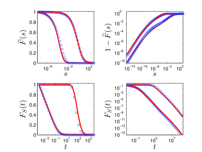
Figure 7: In this graph a comparison between the analytic approximation (47) and the numerical results for a Gaussian disorder is shown in Laplace (top) and time (bottom) spaces. The parameters for these plots are: $E=0.01$, $\sigma=0.3$ and $d=250$, such that $\mu=0.2222$ Circles represent the choice $i_{0}=1$ while squares represent the choice $i_{0}=50$ cases on both, left and right, figures. The red lines are analytic approximations based on Eq. (47).

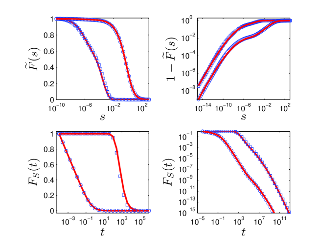
Figure 8: In this graph a comparison between the analytic approximation (47) and the numerical results for a Gaussian disorder is shown in Laplace (top) and time (bottom) spaces. The parameters for these plots are: $E=-0.01$, $\sigma=0.2$ and $d=350$, such that $\mu=-0.5$ Circles represent the choice $i_{0}=1$ while squares represent the choice $i_{0}=50$ cases on both, left and right, figures. The red lines are analytic approximations based on Eq. (47).

VI Summary

In this paper we presented a random tilt model and solved it analytically. We showed that the model can be used to obtain an approximate expression for the FPT distribution of a random walker on a random forcing energy landscape. To do this several parameters of the RT model have to be set as a function of the RF model parameters. As we showed, this can be done with no free fitting parameters. For convenience we summarize the results below.

The approximation for the random walker’s Laplace transformed FPT probability density from site $i_{0}>0$ to the origin on a random forcing energy landscape with i.i.d. random variables $\left\{p_{i}\right\}$ and $\left\{q_{i}\right\}$ is:

$$\widetilde{F}\left(s\right)=\int_{-\infty}^{\infty}\frac{e^{-d\frac{\left(\varepsilon-\left\langle\varepsilon\right\rangle\right)^{2}}{2\sigma_{\varepsilon}^{2}}}}{\sqrt{2\pi\frac{\sigma_{\varepsilon}^{2}}{d}}}\left[\pi_{1}\Phi\left(\frac{s}{v_{1}},\varepsilon\right)+\pi_{2}\Phi\left(\frac{s}{v_{2}},\varepsilon\right)+\left(1-\pi_{2}-\pi_{3}\right)\Phi\left(\frac{s}{v_{3}},\varepsilon\right)\right]d\varepsilon\text{ (Eq. (\ref{10})),}$$

where

$$\Phi\left(\frac{s}{v},\varepsilon\right)=\frac{\lambda_{2}^{i_{0}}\left(\frac{s}{v},\varepsilon\right)}{2^{i_{0}}}\frac{1-\left(\frac{\lambda_{2}\left(\frac{s}{v},\varepsilon\right)}{\lambda_{1}\left(\frac{s}{v},\varepsilon\right)}\right)^{d-i_{0}-1}\frac{\left(\frac{s}{v}+1\right)\lambda_{2}\left(\frac{s}{v},\varepsilon\right)-2}{\left(\frac{s}{v}+1\right)\lambda_{1}\left(\frac{s}{v},\varepsilon\right)-2}}{1-\left(\frac{\lambda_{2}\left(\frac{s}{v},\varepsilon\right)}{\lambda_{1}\left(\frac{s}{v},\varepsilon\right)}\right)^{d-1}\frac{\left(\frac{s}{v}+1\right)\lambda_{2}\left(\frac{s}{v},\varepsilon\right)-2}{\left(\frac{s}{v}+1\right)\lambda_{1}\left(\frac{s}{v},\varepsilon\right)-2}}\text{ (Eq. (\ref{31})),}$$

$$\lambda_{1,2}\left(\frac{s}{v},\varepsilon\right)=1+\left(1+\frac{s}{v}\right)e^{\varepsilon}\pm\sqrt{1+2e^{\varepsilon}\left(\frac{s}{v}-1\right)+e^{2\varepsilon}\left(\frac{s}{v}+1\right)^{2}}\text{ (Eq. (\ref{25})),}$$

$$\left\langle\overline{t}\right\rangle=\left\langle\frac{1}{q_{i}}\right\rangle\frac{\left\langle e^{-E_{i}}\right\rangle^{d+1}-\left\langle e^{-E_{i}}\right\rangle^{d-i_{0}+1}}{\left(\left\langle e^{-E_{i}}\right\rangle-1\right)^{2}}-\left\langle\frac{1}{q_{i}}\right\rangle\frac{i_{0}}{\left\langle e^{-E_{i}}\right\rangle-1}\text{(Eq. (\ref{19})),}$$

$$I=\int_{-\infty}^{\infty}\left[\frac{e^{-\varepsilon\left(d+1\right)}-e^{-\varepsilon\left(d-i_{0}+1\right)}}{\left(e^{-\varepsilon}-1\right)^{2}}-\frac{i_{0}}{e^{-\varepsilon}-1}\right]\frac{e^{-d\frac{\left(\varepsilon-\left\langle\varepsilon\right\rangle\right)^{2}}{2\sigma_{\varepsilon}^{2}}}}{\sqrt{2\pi\frac{\sigma_{\varepsilon}^{2}}{d}}}d\varepsilon\text{ (Eq. (\ref{13})),}$$

$$v_{1}=\frac{I}{\left\langle\overline{t}\right\rangle}\text{ (Eq. (\ref{28})),}$$

$$v_{2}=\left\langle q_{i}\right\rangle\text{ (Eq. (\ref{29}))},$$

$$v_{3}=\left\langle\frac{1}{q_{i}}\right\rangle^{-1}\text{ (Eq. (\ref{30})),}$$

$$\pi_{1}=\frac{v_{1}\left\langle\overline{t}\right\rangle}{I}\frac{v_{2}v_{3}\left(v_{2}^{i_{0}}-v_{3}^{i_{0}}\right)+\frac{I\left\langle q\right\rangle^{i_{0}}}{\left\langle\overline{t}\right\rangle}\left(v_{2}-v_{3}\right)+\frac{I}{\left\langle\overline{t}\right\rangle}\left(v_{3}^{i_{0}+1}-v_{2}^{i_{0}+1}\right)}{v_{2}v_{3}\left(v_{2}^{i_{0}}-v_{3}^{i_{0}}\right)+v_{1}^{i_{0}+1}\left(v_{2}-v_{3}\right)+v_{1}\left(v_{3}^{i_{0}+1}-v_{2}^{i_{0}+1}\right)}\text{ (Eq. (\ref{26})),}$$

$$\pi_{2}=-\frac{v_{2}\left\langle\overline{t}\right\rangle}{I}\frac{v_{1}v_{3}\left(v_{1}^{i_{0}}-v_{3}^{i_{0}}\right)+\frac{I\left\langle q\right\rangle^{i_{0}}}{\left\langle\overline{t}\right\rangle}\left(v_{1}-v_{3}\right)+\frac{I}{\left\langle\overline{t}\right\rangle}\left(v_{3}^{i_{0}+1}-v_{1}^{i_{0}+1}\right)}{v_{2}v_{3}\left(v_{2}^{i_{0}}-v_{3}^{i_{0}}\right)+v_{1}^{i_{0}+1}\left(v_{2}-v_{3}\right)+v_{1}\left(v_{3}^{i_{0}+1}-v_{2}^{i_{0}+1}\right)}\text{ (Eq. (\ref{27})),}$$

$$\left\langle\varepsilon\right\rangle=E\text{ (Eq. (\ref{2})) and}$$

$$\sigma_{\varepsilon}=\left\{\begin{array}[c]{cc}\sigma&E\leq 0\\ \sqrt{\frac{2E}{\mu}}&E>0\end{array}\right.\text{ (Eqs. (\ref{22}) and (\ref{7})).}$$

If one is not interested in the large or in the small $s$ behavior one may use the much simpler Eqs. (34) or (38), respectively, instead of Eq. (47).

Comparing this approximation with the numerically calculated FPT distribution of the RF model we showed that the first may serve as a good approximation to the second. Finally, similar methods can be used to approximate other, say absorbing, boundary conditions at $i=d+1$.

- (1) R. Bruinsma and G. Aeppli, Phys. Rev. Lett. 52, 1547 (1984).
- (2) G. Grinstein and J. F. Fernandez, Phys. Rev. B 29, 6389 (1984).
- (3) R. Maynard, J. Phys. Lett. 45, 81 (1984).
- (4) T. Nattermann and J. Villain, Phase Transitions 11, 5 (1988).
- (5) J. P. Harth and J. Lothe, The Theory of Dislocations (McGraw Hill, New York, 1968).
- (6) D. K. Lubensky and D. R. Nelson, Phys. Rev. Lett. 85, 1572 (2000).
- (7) C. Danilowicz, V. W. Coljee, C. Bouzigues, D. K. Lubensky, D. R. Nelson, and M. Prentiss, PNAS 10, 1694 (2003).
- (8) J. D. Weeks, J. B. Lucks, Y. Kafri, C. Danilowicz, D. R. Nelson, and M. Prentiss, Biophys. J. 88, 2752 (2005).
- (9) J. Mathe, H. Visram, V. Viasnoff, Y. Rabin, and A. Meller, Biophys. J. 87, 3205 (2004).
- (10) T. Harms and R. Lipowsky, Phys. Rev. Lett. 79, 2895 (1997).
- (11) Y. Kafri, D. K. Lubensky, and D. R. Nelson, Bioph. J. 86, 3373 (2004).
- (12) Y. Kafri, D. K. Lubensky, and D. R. Nelson, Phys. Rev. E 71, 041906 (2005).
- (13) D. Hexner and Y. Kafri, Phys. Biol. 6, 036016 (2009).
- (14) Y. G. Sinai, Teor. Veroyatnost. i Primenen. 27, 247 (1982).
- (15) B. Derrida, J. Stat. Phys. 31, 433 (1983).
- (16) H. Kesten, M. V. Kozlov, and F. Spitzer, Compositio Math. 30, 145 (1975).
- (17) F. Solomon, Ann. Probab. 3, 1 (1975).
- (18) B. Derrida and Y. Pomeau, Phys. Rev. Lett. 48, 627 (1982).
- (19) J.-P. Bouchaud and A. Georges, Phys. Rep. 195, 127 (1990).
- (20) A. Golosov, Commun. Math. Phys. 92, 491 (1984).
- (21) S.Condamin, O. Benichou, V. Tejedor, R. Voituriez, and J. Klafter, Nature 450, 77 (2007).
- (22) O. Benichou, C. Chevalier, J. Klafter, B. Meyer, and R. Voituriez, Nature Chemistry 2, 472 (2010).
- (23) G. Oshanin and S. Redner, Europhys. Lett. 85, 10008 (2008).
- (24) K. P. N. Murthy and K. W. Kehr, Phys. Rev. A 40, 2082 (1989).
- (25) P. Le Doussal, Phys. Rev. Lett. 62, 3097 (1989).
- (26) P. Le Doussal, C. Monthus, and D. S. Fisher, Phys. Rev. E 59, 4795 (1999).
- (27) I. Lifshitz, S. Gredeskul, and L. Pastur, Introduction into the theory of disordered systems (John Wiley, New York, 1957).
- (28) W. Feller, Wiley Series in Probability and Mathematical Statistics (Wiley, New York, 1957).