Numerical relativity for $D$ dimensional space-times:
Head-on collisions of black holes and gravitational wave extraction

Abstract

Higher dimensional black holes play an exciting role in fundamental physics, such as high energy physics. In this paper, we use the formalism and numerical code reported in Zilhao:2010sr to study the head-on collision of two black holes. For this purpose we provide a detailed treatment of gravitational wave extraction in generic $D$ dimensional space-times, which uses the Kodama-Ishibashi formalism. For the first time, we present the results of numerical simulations of the head-on collision in five space-time dimensions, together with the relevant physical quantities. We show that the total radiated energy, when two black holes collide from rest at infinity, is approximately $(0.089\pm 0.006)\%$ of the centre of mass energy, slightly larger than the $0.055\%$ obtained in the four dimensional case, and that the ringdown signal at late time is in very good agreement with perturbative calculations.

I Introduction

Black objects in higher dimensional space-times have a remarkably richer structure than their four dimensional counterparts. They appear in a variety of configurations (e.g. black holes, black branes, black rings, black Saturns), and display complex stability phase diagrams (see Emparan:2008eg for an overview). They might also play a key role in high energy physics: High energy physics scenarios, such as the gauge-gravity duality Maldacena:1997re or TeV gravity models Antoniadis:1990ew ; ArkaniHamed:1998rs ; Antoniadis:1998ig ; Randall:1999ee ; Randall:1999vf , suggest that dynamical processes involving higher dimensional black holes (BHs) may be relevant for understanding the physics under experimental scrutiny at particle colliders, such as the Large Hadron Collider (LHC) or the Relativistic Heavy Ion Collider (RHIC). These processes can be quite violent and highly nonlinear, as in the case of BH collisions. Numerical relativity, which solves Einstein’s equations on supercomputers, is therefore the only available tool for high-precision studies of such BH systems. Fortunately, the field of numerical relativity has matured considerably over the last five years (see Refs. Pretorius:2007nq ; Hinder:2010vn for reviews), and its techniques can now be extended to a much wider class of space-times. Space-times of generic dimensionality or with more general asymptotics, feature most prominently among such generalizations. Recent applications to the study of higher dimensional BH instabilities may be found in Refs. Shibata:2009ad ; Shibata:2010wz , using the formalism developed in Ref. Yoshino:2009xp ; an application to the study of $AdS$-like asymptotics may be found in Ref. Witek:2010qc . Further applications of numerical relativity to more general types of space-times have been discussed in Ref. Zilhao:2010sr , hereafter denoted as Paper I, wherein we have started a long-term effort to evolve BH space-times in higher dimensions numerically, and developed a framework to perform numerical simulations of $D$ dimensional space-times with an $SO(D-2)$ isometry group (for $D\geq 5$) or $SO(D-3)$ (for $D\geq 6$).

One scenario in which BH collisions play a very well defined role is that of TeV-scale gravity, i.e. scenarios in which the fundamental Planck scale is of the order of the TeV. The beginning of the scientific runs at the LHC makes accurate theoretical modelling of the experimental signatures of this scenario for LHC collisions very timely. In this scenario, for centre of mass energies well above the TeV threshold, recall that LHC collisions will reach 14 TeV, parton-parton collision will be dominated by the gravitational interaction, and should be well described by any classical gravitational objects with the same gravitational energy. For modelling simplicity, it is convenient to choose these objects to be BHs Banks:1999gd ; Giddings:2001bu ; Dimopoulos:2001hw ; Feng:2001ib ; Ahn:2003qn ; Ahn:2002mj ; Chamblin:2004zg ; Cardoso:2004zi ; Cavaglia:2002si ; Kanti:2004nr ; Kanti:2008eq ; Solodukhin:2002ui ; Hsu:2002bd . Due to the dominance of the gravitational interaction, we may further neglect the electric charge of the holes; charge dependant effects should give sub-leading corrections to the relevant observables. For sufficiently small impact parameters, these trans-Planckian collisions are expected to form a BH Giddings:2001bu ; Dimopoulos:2001hw , as follows from Thorne’s hoop conjecture Thorne:1972ji which recently has received support from the numerical work of Choptuik and Pretorius Choptuik:2009ww . Therefore, there is substantial evidence that modelling the individual partons as BHs is not biasing the final result of the parton scattering process towards BH formation. Indeed, this is the idea that, above the fundamental Planck scale, matter does not matter; it only matters the gravitational energy that each parton carries.

After formation, the BH should then decay via Hawking evaporation. In order to filter experimental data, this process has been modelled by dedicated Monte Carlo event generators, such as Truenoir, Catfish, Charybdis2 or Blackmax Dimopoulos:2001hw ; Cavaglia:2006uk ; Frost:2009cf ; Dai:2007ki ; Dai:2009by . The latter two are being used by the ATLAS experiment at the LHC. These generators clearly exhibit the very distinct experimental signatures of BH evaporation, including higher multiplicity of jets and larger transverse momentum than those produced by any standard model process Aad:2009wy . The event generators also model the BH production phase from the parton-parton scattering, for which they need as an input the threshold impact parameter for BH formation and the energy lost in gravitational radiation during the parton-parton collision. At the moment, the best estimates for these quantities are based on trapped surface methods Yoshino:2005hi . Accurate results can, however, be obtained from full-blown numerical simulations, as has already been seen in four dimensions Sperhake:2008ga ; Shibata:2008rq ; Sperhake:2009jz . Such results will be instrumental in a more accurate phenomenological modelling of BH production/evaporation in particle colliders. Observe that, even if no evidence for BH formation/evaporation is found at the LHC, such accurate modelling will matter for setting precise lower bounds on the fundamental Planck scale.

In this paper we present the first fully nonlinear treatment of a head-on collision of BHs in a higher dimensional space-time, together with an analysis of the relevant physical quantities. This is achieved by solving the corresponding Einstein equations numerically, for which we use the formalism and code reported in Paper I. Once given the numerically constructed space-time, one is still left with the question of extracting physically meaningful quantities, such as the energy and linear and angular momentum carried away by the gravitational radiation.

In four space-time dimensions, two distinct formalisms have been developed to extract the physical information (see e.g. Ref. Alcubierre:2008 for a review of both formalisms). One is based on the Regge-Wheeler-Zerilli perturbation theory for the Schwarzschild BH Regge:1957td ; Zerilli:1970se ; the other is based on the Newman-Penrose formalism Newman:1961qr , which was used by Teukolsky to study perturbations of algebraically special space-times Teukolsky:1973ha , a class which includes the Kerr BH. A higher dimensional generalization of the Newman-Penrose formalism has been developed in Refs. Coley:2004jv ; Milson:2004jx ; Pravda:2004ka ; Ortaggio:2007eg . Unfortunately, the condition of being algebraically special does not seem to be as powerful for the study of exact solutions or their perturbations in higher dimensions as it was in four dimensions. For instance, the Goldberg-Sachs theorem is not valid any longer in higher dimensions Pravda:2004ka ; Ortaggio:2007eg . For the study we present herein, however, it suffices to use the higher dimensional generalisation of the Regge-Wheeler-Zerilli formalism, because the final result of a head-on collision of two $D$ dimensional, nonspinning BHs approaches, at late times, a $D$ dimensional Schwarzschild, i.e. Tangherlini Tangherlini:1963bw BH. Fortunately, the perturbation theory of the latter BH has been fully developed, in arbitrary dimensions, by Kodama and Ishibashi Kodama:2003jz . Our remaining task is to obtain the relevant gauge-invariant quantities from our numerical data, a procedure that we shall describe in detail in this paper.

After implementing this wave-extraction formalism we apply it to study the head-on collision of two BHs in four and five dimensional space-times. In four dimensions we recover previous results in the literature, and we perform a number of tests on the numerical coordinate system, to ensure it is appropriate for the wave extraction formalism. We estimate that around $0.055\%$ of the centre of mass energy is radiated when two BHs, at rest at infinity, collide. This result is in good agreement with those reported in the literature Sperhake:2006cy . The five dimensional results are entirely new. We show that the kinematics of the BHs before the merging follow, to a good precision, the Newtonian prediction. We estimate that around $0.089\%$ of the centre of mass energy is radiated as gravitational waves, when two BHs collide from rest at infinity, and present the associated waveforms. We stress that these results refer to a fully nonlinear evolution of Einstein’s field equations.

This paper is organized as follows. In Section II we apply the Kodama-Ishibashi (KI) formalism to the space-times considered in Paper I. By assuming that the numerical space-time is a small deviation from the Tangherlini solution, one is able to relate (see relations (II.3)) the numerical metric to the KI metric perturbations and to compute gauge-invariant quantities using Eqs. (28), (29). These are then used to construct a master function $\Phi$ (see Eq. (54)) from which all relevant information about the radiation can be computed. In Sections III, IV we present results obtained from the evolution of Brill-Lindquist initial data in $D=4,~{}5$ respectively, that represents the collision of two equal-mass, nonspinning BHs which are initially at rest. In order to calibrate the accuracy of the wave extraction formalism, we perform a number of tests, including tests on the numerical coordinates themselves. We compute the time derivative of the master function $\Phi$, energy fluxes and total energy radiated. We give some final remarks in Sec. V and discuss future steps in this research program. Two appendices cover technical details on the coordinate transformation between the numerical and wave extraction frames (Appendix A) and on the $D$ dimensional harmonic expansion of axisymmetric tensors (Appendix B).

II Gravitational wave extraction in $D$ dimensional axially symmetric space-times

II.1 Coordinate frames

In the approach developed in Paper I, we perform a dimensional reduction by isometry on the $(D-4)$-sphere $S^{D-4}$, in such a way that the $D$ dimensional vacuum Einstein equations are rewritten as an effective $3+1$ dimensional time evolution problem with source terms that involve a scalar field. The evolution equations are expressed in the Baumgarte-Shapiro-Shibata-Nakamura (BSSN) formulation Shibata:1995we ; Baumgarte:1998te , and numerically implemented using a modification of the Lean code Sperhake:2006cy .

In Paper I we considered different generalizations of “axial symmetries” to higher dimensions: either $D\geq 5$ dimensional space-times with $SO(D-2)$ isometry group, or $D\geq 6$ dimensional space-times with $SO(D-3)$ isometry group. In this work we only study the former case, which allows us to model head-on collisions of nonspinning BHs; we dub hereafter these space-times as axially symmetric. Although the corresponding symmetry manifold is the $(D-3)$-sphere $S^{D-3}$, the quotient manifold in our dimensional reduction is its submanifold $S^{D-4}$. The coordinate frame in which the numerical simulations are performed is

$$(x^{\mu},\phi^{1},\dots,\phi^{D-4})=(t,x,y,z,\phi^{1},\dots,\phi^{D-4})\,,$$ (1)

where the angles $\phi^{1},\dots,\phi^{D-4}$ describe the quotient manifold $S^{D-4}$ and do not appear explicitly in the simulations. Here, $z$ is the symmetry axis, i.e. the collision line.

In the frame (1), the space-time metric has the form (cf. Eqs. (2.14) and (2.21) of Paper I)

$$ds^{2}= g_{\mu\nu}(x^{\alpha})dx^{\mu}dx^{\nu}+\lambda(x^{\mu})d\Omega_{D-4}$$

$$= -\alpha^{2}dt^{2}+\gamma_{ij}(dx^{i}+\beta^{i}dt)(dx^{j}+\beta^{j}dt)$$

$$+\lambda(x^{\mu})d\Omega_{D-4}\,,$$ (2)

where $x^{\mu}=(t,x^{i})$, $\lambda(x^{\mu})$ is a scalar field and $\alpha,\beta^{i}$ are the lapse function and the shift vector, respectively. It is worth noting that, although in $D=4$ a general axially symmetric space-time has nonvanishing mixed components of the metric (like $g_{t\phi}$), in $D\geq 5$ such components vanish in an appropriate coordinate frame, as we have shown in Paper I.

With an appropriate transformation of the four dimensional coordinates $x^{\mu}$, the residual symmetry left after the dimensional reduction on $S^{D-4}$ can be made manifest: $x^{\mu}\rightarrow(x^{\bar{\mu}},\theta)$ ($\bar{\mu}=0,1,2$),

$$g_{\mu\nu}(x^{\alpha})dx^{\mu}dx^{\nu}=g_{\bar{\mu}\bar{\nu}}(x^{\bar{\alpha}})dx^{\bar{\mu}}dx^{\bar{\nu}}+g_{\theta\theta}(x^{\bar{\alpha}})d\theta^{2}$$ (3)

and

$$\lambda(x^{\mu})=\sin^{2}\theta g_{\theta\theta}(x^{\bar{\alpha}})\,,$$ (4)

so that Eq. (2) takes the form $ds^{2}=g_{\bar{\mu}\bar{\nu}}dx^{\bar{\mu}}dx^{\bar{\nu}}+g_{\theta\theta}d\Omega_{D-3}$, as discussed in Paper I.

To extract the gravitational waves far away from the symmetry axis we employ the KI formalism Kodama:2003jz , which generalizes the Regge-Wheeler-Zerilli Regge:1957td ; Zerilli:1970se approach to higher dimensions. We require that the space-time, far away from the BHs, is approximately spherically symmetric. Note, that spherical symmetry in $D$ dimensions means symmetry with respect to rotations on $S^{D-2}$; this is an approximate symmetry which holds asymptotically far away from the axis and which is manifest in the coordinate frame:

$$(x^{a},\bar{\theta},\theta,\phi^{1},\dots,\phi^{D-4})=(t,r,\bar{\theta},\theta,\phi^{1},\dots,\phi^{D-4})\,.$$ (5)

Note that $x^{a}=t,r$ and that we have introduced polar-like coordinates $\bar{\theta},\theta\in[0,\pi]$ to “build up” the manifold $S^{D-2}$ in the background, together with a radial spherical coordinate $r$, which is the areal coordinate in the background.

The coordinate frame (5) is defined in such a way that the metric can be expressed as a stationary background $(ds^{(0)})^{2}$ (i.e., the Tangherlini metric) plus a perturbation $(ds^{(1)})^{2}$ which decays faster than $1/r^{D-3}$ for large $r$:

$$(ds^{(0)})^{2}= g^{(0)}_{ab}dx^{a}dx^{b}+r^{2}d\Omega_{D-2}$$

$$= g_{tt}^{(0)}dt^{2}+g_{rr}^{(0)}dr^{2}+r^{2}d\Omega_{D-2}$$

$$= g_{tt}^{(0)}dt^{2}+g_{rr}^{(0)}dr^{2}+r^{2}\left(d\bar{\theta}^{2}+\sin^{2}\bar{\theta}d\Omega_{D-3}\right)$$

$$= -\left(1-\frac{r_{S}^{D-3}}{r^{D-3}}\right)dt^{2}+\left(1-\frac{r_{S}^{D-3}}{r^{D-3}}\right)^{-1}dr^{2}$$

$$+r^{2}\left[d\bar{\theta}^{2}+\sin^{2}\bar{\theta}\left(d\theta^{2}+\sin^{2}\theta d\Omega_{D-4}\right)\right]\,,$$ (6)

$$(ds^{(1)})^{2}= h_{ab}dx^{a}dx^{b}+h_{a\bar{\theta}}dx^{a}d\bar{\theta}+h_{\bar{\theta}\bar{\theta}}d\bar{\theta}^{2}$$

$$+h_{\theta\theta}d\Omega_{D-3}\,.$$ (7)

Here, the Schwarzschild radius $r_{S}$ replaces the parameter $\mu$ used in Paper I and is related to the Arnowitt-Deser-Misner mass $M$ by

$$r_{S}^{D-3}=\frac{16\pi M}{(D-2){\cal A}_{D-2}}\,,$$ (8)

where ${\cal A}_{D-2}$ is the area of the $(D-2)$-sphere (see Eq. (100)). For instance, $r_{S}=2M$ in $D=4$ and $r_{S}=\sqrt{8M/(3\pi)}$ in $D=5$.

When we define the coordinate frame (5), we also require that the coordinate $\theta$ in this frame coincides with the coordinate $\theta$ appearing in Eq. (3). With this choice, the axial symmetry of the space-time implies that

$$h_{a\theta}=h_{\bar{\theta}\theta}=0\,,$$ (9)

as in Eq. (7), and $\lambda=\sin^{2}\theta g_{\theta\theta}$, i.e. Eq. (4).

The transformation from the coordinates $x^{\mu}=(t,x,y,z)$ in which the numerical simulation is implemented to the coordinates $(x^{a},\bar{\theta},\theta)=(t,r,\bar{\theta},\theta)$ in which the wave extraction is performed is given by

$$x =R\sin\bar{\theta}\cos\theta\,,$$ (10)

$$y =R\sin\bar{\theta}\sin\theta\,,$$ (11)

$$z =R\cos\bar{\theta}\,,$$ (12)

where $R=\sqrt{x^{2}+y^{2}+z^{2}}$ and by the reparametrization of the radial coordinate

$$R=R(r)\,.$$ (13)

We note that Eqs. (12), (13) correctly transform the three-metric $\gamma_{ij}$ describing the initial data

$$\gamma_{ij}dx^{i}dx^{j}=\psi^{\frac{4}{D-3}}(dR^{2}+R^{2}(d{\bar{\theta}}^{2}+\sin^{2}\bar{\theta}d\theta^{2}))\,,$$ (14)

where, as discussed in Paper I, we choose Brill-Lindquist initial data,

$$\psi=1+\frac{r_{S,1}^{D-3}}{4r_{1}^{D-3}}+\frac{r_{S,2}^{D-3}}{4r_{2}^{D-3}}\,,$$ (15)

in order to simulate a head-on collision of BHs starting from rest. Here, $r_{S,i}$ and $r_{i}$ denote the Schwarzschild radius and the initial position of the $i$-th BH, respectively. Far away from the axis the conformal factor is given by $\psi\rightarrow 1+\hbox{ perturbations}$. Therefore, the splitting of the metric into a Tangherlini background plus a perturbation, Eqs. (6)-(7), can be recovered on the initial time-slice, if we define the reparametrization (13) appropriately.

Our guess is that the transformation (12), (13) yields the “Tangherlini+perturbation” splitting (6), (7) during the entire evolution of the system. This statement can be checked numerically by verifying the following relations (see Appendix B):

$$\mathcal{G}_{tt} \equiv\frac{1}{K^{0D}\pi}\int_{0}^{\pi}d\bar{\theta}\sin^{D-3}\bar{\theta}\int_{0}^{\pi}d\theta g_{tt}(\bar{\theta},\theta)-g_{tt}^{(0)}=0\,,$$ (16)

$$\mathcal{G}_{tr} \equiv\frac{1}{K^{0D}\pi}\int_{0}^{\pi}d\bar{\theta}\sin^{D-3}\bar{\theta}\int_{0}^{\pi}d\theta g_{tR}(\bar{\theta},\theta)=0\,,$$ (17)

$$\mathcal{G}_{rr} \equiv\frac{1}{K^{0D}\pi}\int_{0}^{\pi}d\bar{\theta}\sin^{D-3}\bar{\theta}\int_{0}^{\pi}d\theta g_{RR}(\bar{\theta},\theta)-g_{rr}^{(0)}=0\,,$$ (18)

where $K^{0D}=\int_{0}^{\pi}d\bar{\theta}(\sin\bar{\theta})^{D-3}$, together with the axisymmetry conditions (4), (9). As we will discuss in Section III, Eqs. (4), (9), (16)–(18) are indeed satisfied with high accuracy throughout the numerical evolution. The preservation of the above identities during the numerical evolution justifies also the identification of the time coordinate in the numerical and wave extraction frames, and our use of the KI formalism.

Finally, Eqs. (2), (6), (7) yield the $3+1$ splitting

$$ds^{2}= (ds^{(0)})^{2}+(ds^{(1)})^{2}$$

$$= g_{\bar{\mu}\bar{\nu}}dx^{\bar{\mu}}dx^{\bar{\nu}}+(r^{2}\sin^{2}\bar{\theta}+h_{\theta\theta})d\Omega_{D-3}$$

$$= g_{\bar{\mu}\bar{\nu}}dx^{\bar{\mu}}dx^{\bar{\nu}}+(r^{2}\sin^{2}\bar{\theta}+h_{\theta\theta})$$

$$\times(d\theta^{2}+\sin^{2}\theta d\Omega_{D-4})$$

$$= -\alpha^{2}dt^{2}+\gamma_{ij}(dx^{i}+\beta^{i}dt)$$

$$\times(dx^{j}+\beta^{j}dt)+\lambda d\Omega_{D-4}\,,$$ (19)

where $x^{\bar{\mu}}=(t,r,\bar{\theta})$. With the $3+1$ splitting, the axisymmetry conditions (4), (9) take the form

$$\lambda=\gamma_{\theta\theta}\sin^{2}\theta\,,~{}~{}~{}~{}~{}\gamma_{R\theta}=\gamma_{\bar{\theta}\theta}=\beta^{\theta}=0\,.$$ (20)

The variable $r$ can be determined from the angular components of the metric (II.1), by averaging out $h_{\bar{\theta}\bar{\theta}}$, $h_{\theta\theta}$ (see Appendix B); its explicit expression is given by

$$(r(R))^{2}= \frac{1}{(D-2)K^{0D}}\int_{0}^{\pi}d\bar{\theta}\left[\gamma_{\bar{\theta}\bar{\theta}}(\sin\bar{\theta})^{D-3}\right.$$

$$\left.+(D-3)\gamma_{\theta\theta}(\sin\bar{\theta})^{D-5}\right]\,.$$ (21)

As we will discuss in Section III, we find that the areal radius $r$ is very close to $R$.

II.2 Harmonic expansion

In the KI formalism Kodama:2003jz (see also Kodama:2000fa ), the background space-time has the form (6)

$$(ds^{(0)})^{2}= g^{(0)}_{AB}dx^{A}dx^{B}=g^{(0)}_{ab}dx^{a}dx^{b}+r^{2}d\Omega_{D-2}$$

$$= g^{(0)}_{ab}dx^{a}dx^{b}+r^{2}\gamma_{\bar{i}\bar{j}}d\phi^{\bar{i}}d\phi^{\bar{j}}\,,$$ (22)

i.e. the Tangherlini metric, where the $x^{A}$ coordinates refer to the full space-time. The space-time perturbations can be decomposed into spherical harmonics on the $(D-2)$-sphere $S^{D-2}$. They are functions of the $D-2$ angles $\phi^{\bar{i}}=(\bar{\theta},\theta,\phi^{1},\dots,\phi^{D-4})$. We denote the metric of $S^{D-2}$ by $\gamma_{\bar{i}\bar{j}}$, and with a subscript ${}_{:\bar{i}}$ the covariant derivative with respect to this metric. Finally, we denote the covariant derivative with respect to the metric $g^{(0)}_{ab}$ with a subscript _|a.

As discussed in Kodama:2003jz , there are three types of spherical harmonics:

• The scalar harmonics ${\cal S}(\phi^{\bar{i}})$, which are solutions of

  $$\Box{\cal S}=\gamma^{\bar{i}\bar{j}}{\cal S}_{:\bar{i}\bar{j}}=-k^{2}{\cal S}\,,$$ (23)

  with $k^{2}=l(l+D-3)$, $l=0,1,2,\dots$ . The scalar harmonics ${\cal S}$ depend on the integer $l$ and on other indices; we leave such dependence implicit. We also define

  $${\cal S}_{\bar{i}}= -\frac{1}{k}{\cal S}_{,\bar{i}}\,,\,\,{\cal S}_{\bar{i}\bar{j}}=\frac{1}{k^{2}}{\cal S}_{:\bar{i}\bar{j}}+\frac{1}{D-2}\gamma_{\bar{i}\bar{j}}{\cal S}\,.$$ (24)

  Observe that $\gamma^{\bar{i}\bar{j}}{\cal S}_{\bar{i}\bar{j}}=0$.

  Each harmonic mode of the metric perturbation $\delta g_{MN}=h_{MN}$ can be decomposed as

  $$\delta g_{ab}=h_{ab} = f_{ab}{\cal S}\,,$$ (25)

  $$\delta g_{a\bar{i}}=h_{a\bar{i}} = rf_{a}{\cal S}_{\bar{i}}\,,$$ (26)

  $$\delta g_{\bar{i}\bar{j}}=h_{\bar{i}\bar{j}} = 2r^{2}(H_{L}\gamma_{\bar{i}\bar{j}}{\cal S}+H_{T}{\cal S}_{\bar{i}\bar{j}})\,,$$ (27)

  where $f_{ab}$, $f_{a}$, $H_{L}$, $H_{T}$ are functions of $x^{a}=(t,r)$. Note, that in each of these expressions there is a sum over the indices of the harmonic.

  For $l>1$, the metric perturbations can be expressed in terms of the following gauge-invariant variables Kodama:2000fa

  $$F = H_{L}+\frac{1}{D-2}H_{T}+\frac{1}{r}X_{a}r^{|a}\,,$$

  $$F_{ab} = f_{ab}+X_{a|b}+X_{b|a}\,,$$ (28)

  where we have defined

  $$X_{a}=\frac{r}{k}\left(f_{a}+\frac{r}{k}H_{T|a}\right)\,.$$ (29)

• The vector harmonics ${\cal V}_{\bar{i}}(\phi^{\bar{i}})$, solutions of

  $$\gamma^{\bar{i}\bar{j}}{\cal V}_{\bar{k}:\bar{i}\bar{j}}=-k_{V}^{2}{\cal V}_{\bar{k}}\,,$$ (30)

  with $k_{V}^{2}=l(l+D-3)-1$, $l=1,2,\dots$. These harmonics satisfy the relation

  $${\cal V}^{\bar{i}}_{:\bar{i}}=0\,.$$ (31)

  The harmonic expansion of the corresponding metric perturbations is given by Eqs. (26)-(27), with ${\cal S}_{\bar{i}}$ replaced by ${\cal V}_{\bar{i}}$, ${\cal S}_{\bar{i}\bar{j}}$ replaced by

  $${\cal V}_{\bar{i}\bar{j}}=-\frac{1}{2k_{V}}(V_{\bar{i}:\bar{j}}+V_{\bar{j}:\bar{i}})\,,$$ (32)

  and $H_{L}=0$.

• The tensor harmonics ${\cal T}_{\bar{i}\bar{j}}(\phi^{\bar{i}})$, solutions of

  $$\gamma^{\bar{i}\bar{j}}{\cal T}_{\bar{r}\bar{s}:\bar{i}\bar{j}}=-k_{T}^{2}{\cal T}_{\bar{r}\bar{s}}\,,$$ (33)

  with $k_{T}^{2}=l(l+D-3)-2$, $l=1,2,\dots$. These harmonics satisfy,

  $$\gamma^{\bar{i}\bar{j}}{\cal T}_{\bar{i}\bar{j}}=0\,,~{}~{}~{}~{}~{}{\cal T}^{:\bar{i}\bar{j}}_{:\bar{j}}=0\,.$$ (34)

  In the $D=4$ case they vanish. The harmonic expansion of the corresponding metric perturbations is given by (27), with ${\cal S}_{\bar{i}\bar{j}}$ replaced by ${\cal T}_{\bar{i}\bar{j}}$ and $H_{L}=0$.

II.3 Implementation of axisymmetry

In an axially symmetric space-time, the metric perturbations are symmetric with respect to $S^{D-3}$. Therefore, the harmonics in the expansion of $h_{MN}$ depend only on the angle $\bar{\theta}$ (which does not belong to $S^{D-3}$). Furthermore, since there are no off-diagonal terms in the metric (cf. Paper I), the only nonvanishing $g_{a\bar{i}}$ components are $g_{a\bar{\theta}}$; the only components $g_{\bar{i}\bar{j}}$ are either proportional to $\gamma_{\bar{i}\bar{j}}$, or all vanishing but $g_{\bar{\theta}\bar{\theta}}$. This implies that only scalar spherical harmonics can appear in the expansion of the metric perturbations. Indeed, if

$${\cal V}^{\bar{i}}=({\cal V}^{\bar{\theta}},0,\dots,0)\,,~{}~{}~{}~{}~{}{\cal V}^{\bar{i}}={\cal V}^{\bar{i}}(\bar{\theta})\,,$$ (35)

then Eq. (31) gives

$${\cal V}^{\bar{i}}_{:\bar{i}}={\cal V}^{\bar{\theta}}_{,\bar{\theta}}=0~{}~{}~{}\Rightarrow~{}~{}~{}{\cal V}^{\bar{\theta}}=0~{}~{}\Rightarrow~{}~{}~{}{\cal V}^{\bar{i}}=0\,.$$ (36)

Similarly, from Eq. (34) we obtain ${\cal T}_{\bar{i}\bar{j}}=0$.

The scalar harmonics, solutions of Eq. (23) and which depend only on the coordinate $\bar{\theta}$, are given by the Gegenbauer polynomials $C_{l}^{(D-3)/2}$, as discussed in Refs. Berti:2003si ; Cardoso:2002ay ; Yoshino:2005ps ; writing explicitly the index $l$, they take the form

$${\cal S}_{l}(\bar{\theta})=(K^{lD})^{-1/2}C_{l}^{(D-3)/2}(\cos\bar{\theta})\,,$$ (37)

where the normalization $K^{lD}$ is chosen such that

$$\int d\Omega^{D-2}{\cal S}_{l}{\cal S}_{l^{\prime}}=\delta_{ll^{\prime}}\,,~{}~{}~{}\int d\Omega^{D-2}{\cal S}_{l\,,\bar{\theta}}{\cal S}_{l^{\prime}\,,\bar{\theta}}=\delta_{ll^{\prime}}k^{2}\ ,$$ (38)

and $k^{2}=l(l+D-3)$ (see Appendix B). By computing ${\cal S}_{l\,\bar{i}}$, ${\cal S}_{l\,\bar{i}\bar{j}}$ from Eqs. (24) (using Eq. (23)) we find

$${\cal S}_{l\,\bar{\theta}\bar{\theta}} =\frac{D-3}{k^{2}(D-2)}{\cal W}_{l}\,,$$ (39)

$${\cal S}_{l\,\theta\theta} =-\frac{\sin^{2}\bar{\theta}}{k^{2}(D-2)}{\cal W}_{l}\,,$$ (40)

where we have defined

$${\cal W}_{l}(\bar{\theta})={\cal S}_{l\,,\bar{\theta}\bar{\theta}}-\cot\bar{\theta}{\cal S}_{l\,,\bar{\theta}}\,.$$ (41)

Therefore, the metric perturbations are given by

$$h_{ab}= f^{l}_{ab}{\cal S}_{l}(\bar{\theta})\,,$$ (42)

$$h_{a\bar{\theta}}= rf^{l}_{a}{\cal S}_{l}(\bar{\theta})_{\bar{\theta}}=-\frac{1}{k}rf^{l}_{a}{\cal S}_{l}(\bar{\theta})_{,\bar{\theta}}\,,$$ (43)

$$h_{\bar{\theta}\bar{\theta}}= 2r^{2}(H^{l}_{L}{\cal S}_{l}(\bar{\theta})+H^{l}_{T}{\cal S}_{l}(\bar{\theta})_{\bar{\theta}\bar{\theta}})$$

$$= 2r^{2}\left(H^{l}_{L}{\cal S}_{l}(\bar{\theta})+H^{l}_{T}\frac{D-3}{k^{2}(D-2)}{\cal W}_{l}(\bar{\theta})\right)\,,$$ (44)

$$h_{\theta\theta}= 2r^{2}(H^{l}_{L}\sin^{2}\bar{\theta}{\cal S}_{l}(\bar{\theta})+H^{l}_{T}{\cal S}_{l}(\bar{\theta})_{\theta\theta})$$

$$= 2r^{2}\sin^{2}\bar{\theta}\left(H^{l}_{L}{\cal S}_{l}(\bar{\theta})-H^{l}_{T}\frac{1}{k^{2}(D-2)}{\cal W}_{l}(\bar{\theta})\right)\,.$$ (45)

The quantities $f_{ab}$, $f_{a}$, $H_{L}$, $H_{T}$ are (see Appendix B):

$$f^{l}_{ab}(t,r)= \frac{{\cal A}_{D-3}}{\sqrt{K^{lD}}}\int_{0}^{\pi}d\bar{\theta}(\sin\bar{\theta})^{D-3}h_{ab}C_{l}^{(D-3)/2}\,,$$ (46)

$$f_{a}(t,r)= -\frac{1}{\sqrt{l(l+D-3)}r}\frac{{\cal A}_{D-3}}{\sqrt{K^{lD}}}$$

$$\times\int_{0}^{\pi}d\bar{\theta}(\sin\bar{\theta})^{D-3}h_{a\bar{\theta}}C_{l\,,\bar{\theta}}^{(D-3)/2}(\cos{\bar{\theta}})\,,$$ (47)

$$H_{L}(t,r)= \frac{1}{2(D-2)r^{2}}\frac{{\cal A}_{D-3}}{\sqrt{K^{lD}}}\int_{0}^{\pi}d\bar{\theta}(\sin\bar{\theta})^{D-3}$$

$$\times\left[h_{\bar{\theta}\bar{\theta}}+\frac{D-3}{\sin^{2}\bar{\theta}}h_{\theta\theta}\right]C_{l}^{(D-3)/2}(\cos{\bar{\theta}})\,,$$ (48)

$$H_{T}(t,r)= \frac{1}{2r^{2}(k^{2}-D+2)}\frac{{\cal A}_{D-3}}{\sqrt{K^{lD}}}\int_{0}^{\pi}d\bar{\theta}(\sin\bar{\theta})^{D-3}$$

$$\times\left[h_{\bar{\theta}\bar{\theta}}-\frac{1}{\sin^{2}\bar{\theta}}h_{\theta\theta}\right]W_{l}(\bar{\theta})\,,$$ (49)

where $h_{ab}=h_{ab}(t,r,\bar{\theta})$, $h_{a\bar{\theta}}=h_{a\bar{\theta}}(t,r,\bar{\theta})$, $h_{\bar{\theta}\bar{\theta}}=h_{\bar{\theta}\bar{\theta}}(t,r,\bar{\theta})$, $h_{\theta\theta}=h_{\theta\theta}(t,r,\bar{\theta})$ and $C_{l}^{(D-3)/2}=C_{l}^{(D-3)/2}(\cos{\bar{\theta}})$.

In terms of these quantities, using Eqs. (28), (29), we get the gauge-invariant quantities $F$, $F_{ab}$.

As we have discussed above, this approach has been developed for $D>4$, since in $D=4$ the off-diagonal terms $g_{t\phi}$, $g_{r\phi}$ are not vanishing in general axially symmetric space-times. However, we can extend our framework to $D=4$ if we restrict ourselves to axially symmetric space-times with $g_{t\phi}=g_{r\phi}=0$. In this way, we can test our formalism by comparing our results to the existing literature. For instance, we note that in $D=4$ the perturbation functions are related to the expressions in Ref. Sperhake:2005uf , with the identifications

$$f^{l}_{ab} = H_{0},\,H_{1},\,H_{2}\,,$$ (50)

$$-\frac{r}{k}f^{l}_{a} = h_{0},\,h_{1}\,,$$ (51)

$$\frac{2H_{T}}{k^{2}} = G\,,$$ (52)

$$2H_{L}+H_{T} = K\,.$$ (53)

We also remark that in the transverse-traceless gauge, only $H_{T}$ is nonvanishing, but in a generic gauge (like the one used in the numerical simulations) all these quantities are in principle nonvanishing.

II.4 Extracting gravitational waves at infinity

In the KI framework, the emitted gravitational waves are described by the master function $\Phi$. To compute $\Phi$ in terms of the gauge-invariant quantities $F$, $F_{ab}$ one should perform a Fourier transform or a time integration (see Kodama:2003jz ). This can be avoided if we compute directly $\Phi_{,t}$, given by

$$\Phi_{,t}=(D-2)r^{(D-4)/2}\frac{-F^{r}_{~{}t}+2rF_{,t}}{k^{2}-D+2+\frac{(D-2)(D-1)}{2}\frac{r_{S}^{D-3}}{r^{D-3}}}\,,$$ (54)

where $k^{2}=l(l+D-3)$. In the TT-gauge, the gravitational perturbation is described by $H_{T}$, which decays as $r^{(D-2)/2}$ with increasing $r$, whereas the other perturbation functions have a faster decay (see Berti:2003si ). In this gauge, the asymptotic behaviour of the master function is

$$\Phi\simeq\frac{2r^{(D-2)/2}H_{T}}{k^{2}}\,,$$ (55)

and tends to an oscillating function with constant amplitude as $r\rightarrow\infty$. The asymptotic behaviour of $\Phi$ has been checked numerically (cf. Section III).

Writing the index $l$ explicitly, the energy flux in each $l-$multipole is Berti:2003si

$$\frac{dE_{l}}{dt}=\frac{1}{32\pi}\frac{D-3}{D-2}k^{2}(k^{2}-D+2)(\Phi^{l}_{,t})^{2}\,.$$ (56)

The total energy emitted in the process is then

$$E=\sum_{l=2}^{\infty}\int_{-\infty}^{+\infty}dt\frac{dE_{l}}{dt}\,.$$ (57)

III Head-on collision from rest in $D=4$

The numerical simulations of head-on collisions of equal-mass binaries starting from rest have been performed with the Lean code originally introduced in Ref. Sperhake:2006cy , modified along Sec. III of Ref. Sperhake:2007gu and adapted to higher dimensional space-times in Paper I. The Lean code is based on the Cactus computational toolkit cactus and uses the Carpet mesh refinement package Schnetter:2003rb ; carpet , the apparent horizon finder AHFinderDirect Thornburg:1995cp ; Thornburg:2003sf and the puncture initial data solver of Ref. Ansorg:2004ds . Head-on collisions in four dimensional space-times have been studied extensively in the literature and provide valuable opportunities to calibrate the wave extraction formalism. These tests are the subject of the remainder of this Section, while we discuss our new results for five dimensional space-times in Sec. IV below.

Table 1: Grid structure and initial parameters of the head-on collisions starting from rest in $D=4$ and $D=5$. The grid setup is given in terms of the “radii” of the individual refinement levels, in units of $r_{S}$, as well as the resolution near the punctures $h$ (see Sec. II E in Sperhake:2006cy for details). $d$ is the initial coordinate separation of the two punctures and $L$ denotes the proper initial separation.

Run	$D$	Grid Setup	$d/r_{S}$	$L/r_{S}$
HD4c	4	$\{(128,64,32,16,8)\times(1,0.5,0.25),~{}h=r_{S}/80\}$	$5.257$	$7.154$
HD4m	4	$\{(128,64,32,16,8)\times(1,0.5,0.25),~{}h=r_{S}/88\}$	$5.257$	$7.154$
HD4f	4	$\{(128,64,32,16,8)\times(1,0.5,0.25),~{}h=r_{S}/96\}$	$5.257$	$7.154$
HD5a	5	$\{(256,128,64,32,16,8,4)\times(0.5,0.25),~{}h=r_{S}/84\}$	$1.57$	$1.42$
HD5b	5	$\{(256,128,64,32,16,8,4)\times(0.5,0.25),~{}h=r_{S}/84\}$	$1.99$	$1.87$
HD5c	5	$\{(256,128,64,32,16,8,4)\times(1,0.5),~{}h=r_{S}/84\}$	$2.51$	$2.41$
HD5d	5	$\{(256,128,64,32,16,8,4)\times(1,0.5),~{}h=r_{S}/84\}$	$3.17$	$3.09$
HD5ec	5	$\{(256,128,64,32,16,8)\times(2,1,0.5),~{}h=r_{S}/60\}$	$6.37$	$6.33$
HD5em	5	$\{(256,128,64,32,16,8)\times(2,1,0.5),~{}h=r_{S}/72\}$	$6.37$	$6.33$
HD5ef	5	$\{(256,128,64,32,16,8)\times(2,1,0.5),~{}h=r_{S}/84\}$	$6.37$	$6.33$
HD5f	5	$\{(256,128,64,32,16,8)\times(2,1,0.5),~{}h=r_{S}/84\}$	$10.37$	$10.35$

In order to test our implementation of the KI formalism in $D=4$, we have simulated head-on collision of an equal-mass, non spinning BH binary initially at rest. The parameters used in this simulation are shown in Table 1. This particular system is well understood and enables us to compare our results derived from the KI formalism against those obtained using both, the Regge-Wheeler-Zerilli wave extraction and the Newman-Penrose framework; cf. Sperhake:2005uf and Sperhake:2006cy for corresponding literature studies.

In order to perform these tests, we need to relate our master function $\Phi$ of Sec. II.4 to the variables used in traditional four dimensional studies. Specifically, a straightforward calculation shows that the Zerilli wavefunction $\bar{\Phi}$ adopted in Ref. Sperhake:2005uf for $l=2$ multipoles and the outgoing Weyl scalar $\Psi_{4}$ used in Sperhake:2006cy can be expressed in terms of $\Phi$ according to

$$\bar{\Phi} = 6\Phi\,,$$ (58)

$$r\Psi_{4} = \sqrt{6}\Phi_{,tt}\,.$$ (59)

Note that the imaginary part of $\Psi_{4}$ vanishes in the case of a head on collision, due to symmetry.

The resolution is $h=r_{S}/96$ for all results reported in this section except for the convergence study in Sec. III.3 which also uses the lower resolutions $h_{c}=r_{S}/80$ and $h_{m}=r_{S}/88$. Gravitational waves have been extracted at three different coordinate radii $R$ (cf. Eq. 13), which we denote by $R_{\rm ex}=30\,r_{S}\,,40\,r_{S}\,,50\,r_{S}$.

III.1 Tests on the numerical coordinates

The procedure described in Section II assumes that the numerical space-time consists of a small deviation from the Schwarzschild-Tangherlini metric. In order to ensure that the gravitational waves are extracted in an appropriate coordinate system we perform a number of checks.

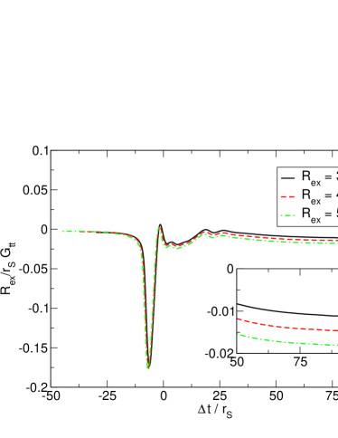
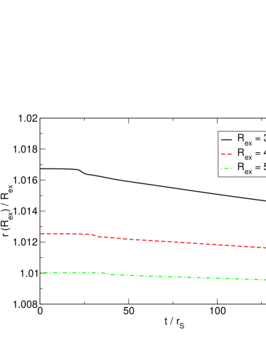
Figure 1: (Color online) Left panel: $\mathcal{G}_{tt}$ calculated from Eq. (16) for $D=4$, at different extraction radii. This quantity has been shifted in time to account for the different extraction radii and re-scaled by the corresponding $R_{\rm ex}$. The late time behavior is shown in the inset. Right panel: time evolution of areal radius (cf. (II.1)) extracted at the radii $R_{\rm ex}=30r_{S}$ (black solid line), $R_{\rm ex}=40r_{S}$ (red dashed line) and $R_{\rm ex}=50r_{S}$ (green dashed-dotted line).

We first test the relations (16), (17) and (18). In Fig. 1 we show $\mathcal{G}_{tt}$, i.e., the difference between the numerical $g_{tt}$, averaged over the extraction sphere and the corresponding component of the assumed background metric. Here we evaluate the background metric by assuming, as a first approximation, that the Schwarzschild radius of the BH is $r_{S}=r_{S,1}+r_{S,2}$.

The deviation of the full 4-metric from the Schwarzschild-Tangherlini background decreases as the extraction radius increases. Indeed, a straightforward calculation shows that a deviation $\delta r_{S}$ of the Schwarzschild radius from the background value leads to $\mathcal{G}_{tt}\sim\delta r_{S}^{D-3}/r^{D-3}$, i. e. $\delta r_{S}/r$ for $D=4$. In the left panel of Fig. 1 we therefore show the deviation $\mathcal{G}_{tt}$ re-scaled by $r$. We further apply a time shift to account for the different propagation time of the wave to reach the extraction radii. As shown in the figure, the deviation from the Schwarzschild line element is small and decreases $\sim 1/r$ in accordance with our expectation. We also note that a deviation $\delta r_{S}$ represents a monopole perturbation of the background which decouples from the quadrupole wave signal at perturbative order, so that its impact on our results is further reduced.

In summary, we can give an uncertainty estimate for the approximation $r_{S}=r_{S,1}+r_{S,2}$ for the Schwarzschild radius of the final BH, which ignores the energy loss through gravitational radiation. As demonstrated by the left panel of Fig. 1, at late times $|R_{\rm ex}/r_{S}\,{\cal G}_{tt}|\sim 0.01$, and, since $r\simeq R_{\rm ex}$ (as we discuss below), we obtain the upper bound

$$\frac{\delta r_{S}}{r_{S}}\lesssim\frac{r}{r_{S}}{\cal G}_{tt}\sim 0.01\,.$$ (60)

This crude analysis sets an upper bound of $\sim 1\%$ on the fraction of the centre of mass energy radiated as gravitational waves. We further note that the close agreement between $g_{tt}$ and its Tangherlini counterpart implies that the time coordinate employed in the numerical simulation and the Tangherlini coordinate time coincide. By analysing $\mathcal{G}_{tr}$ and $\mathcal{G}_{rr}$ in the same manner, we find that relations (16)-(18) are satisfied with an accuracy of one part in $10^{2}$ throughout the evolution, and one part in $10^{3}$ at late times, when the space-time consists of a single distorted black hole.

In practice, gravitational waves are extracted on spherical shells of constant coordinate radius. The significance of the areal radius associated with such a coordinate sphere in the context of extrapolation of GW signals has been studied in detail in Ref. Boyle:2009vi . For our purposes, the most important question is to what extent gauge effects change the areal radius (II.1) of our extraction spheres. For this purpose, we show its time evolution in the right panel of Fig. 1 for different values of $R_{\rm ex}$. The reassuring result is that the areal radius exceeds its coordinate counterpart by about $1~{}\%$ at $R_{\rm ex}=50~{}r_{S}$ and remains nearly constant in time.

III.2 Waveforms

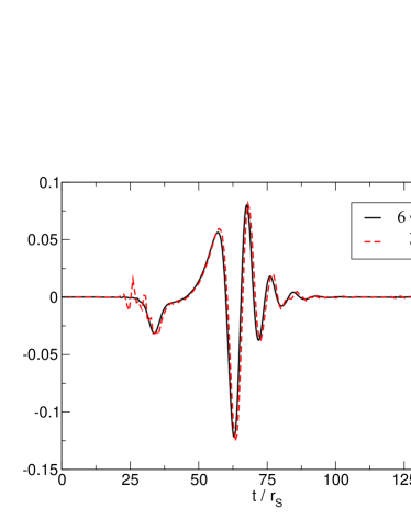
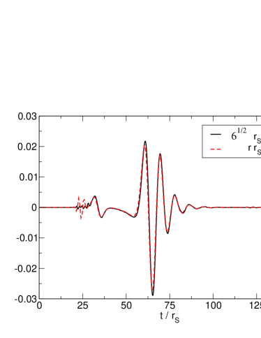
Figure 2: (Color online) Left panel: Time derivatives of the $l=2$ modes of the KI function $\Phi$ (black solid line), and of the Zerilli function $\bar{\Phi}$ (red dashed line) extracted for model HD4_f at $R_{\rm ex}=30r_{S}$. The KI function has been re-scaled by a constant factor (cf. (58)) which accounts for the different normalizations of both formulations. Right panel: comparison of the second time derivative $\Phi_{,tt}$ with the outgoing Newman-Penrose scalar $\Psi_{4}$ for the same model. The KI wavefunction has been re-scaled according to Eq. (59).

As a benchmark for our wave extraction, we compare our results obtained with independent wave extraction tools; (i) the explicitly four dimensional Zerilli formalism and (ii) the Newman-Penrose scalars. For this purpose we have evolved model HD$4_{f}$ and extracted the Zerilli function according to the procedure described in Sperhake:2005uf (see also Eqs. (50) - (53) above) and the Newman Penrose scalar $\Psi_{4}$ as summarized in Sperhake:2006cy . These are compared with the KI wave function $\Phi_{,t}$ and its time derivative $\Phi_{,tt}$ in Fig. 2. Except for a small amount of high frequency noise in the junk radiation at $t\approx 25r_{S}$, we observe excellent agreement between the different extraction methods.

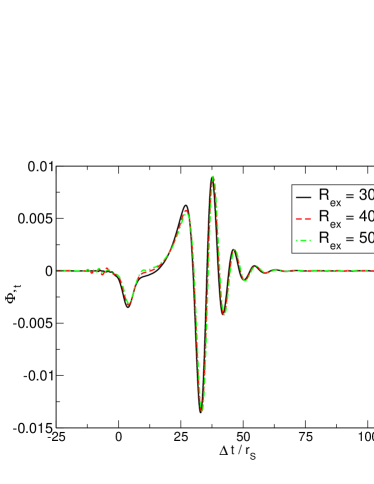
Figure 3: (Color online) The $l=2$ component of the KI wave function $\Phi_{,t}$ extracted at the radii $R_{\rm ex}=30r_{S}$ (black solid line), $R_{\rm ex}=40r_{S}$ (red dashed line) and $R_{\rm ex}=50r_{S}$ (green dashed-dotted line). They have been shifted in time by the corresponding $R_{\rm ex}$.

Next we consider the dependence of the wave signal on the extraction radius. In Fig. 3 we show the $l=2$ component of $\Phi_{,t}$ extracted at three different radii and shifted in time by $R_{\rm ex}$. As is apparent from the figure, the wave function shows little variation with $R_{\rm ex}$ at large distances, in agreement with expectations.

A further test of the wave signal arises from its late-time behaviour which is dominated by the BH ringdown Berti:2009kk , an exponentially damped sinusoid of the form $e^{-{\rm i}\omega t}$, with $\omega$ being a characteristic frequency called quasinormal mode (QNM) frequency. Using well-known methods Berti:2005ys ; Berti:2007dg ; Berti:2009kk , we estimate this frequency to be $r_{S}\,\omega\sim 0.746\pm 0.002-{\rm i}\,(0.176\pm 0.002)$. This can be compared with theoretical predictions from a linearized approach, yielding $r_{S}\,\omega=0.747344-{\rm i}\,0.177925$.

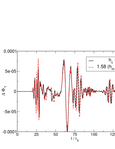
Figure 4: (Color online) Convergence analysis of the $l=2$ component of $\Phi_{,t}$ extracted at $R_{\rm ex}=30\,r_{S}$. We plot the differences between the low and medium resolution (black solid line) and medium and high resolution (red dashed line) run. The latter is re-scaled by the factor $Q=1.58$ expected for $4^{th}$ order convergence Witek:2010qc .

Finally, we consider the numerical convergence of our results. In Fig. 4, we plot the differences obtained for $\Phi_{,t}$ extracted at $R_{\rm ex}=30\,r_{S}$, using the different resolutions of the three models HD$4$ listed in Table 1. The differences thus obtained are consistent with $4^{th}$ order convergence. This implies a discretization error in the $l=2$ component of $\Phi_{,t}$ of about $4\%$ for the grid resolutions used in this work.

III.3 Radiated energy

Once the KI function $\Phi_{,t}$ is known, the energy flux can be computed from Eq. (56). For comparison, we have also determined the flux from the outgoing Newman Penrose scalar $\Psi_{4}$ according to Eq. (22) in Ref. Witek:2010qc . The flux and energy radiated in the $l=2$ multipole, obtained with the two methods at $R_{\rm ex}=50\,r_{S}$ is shown in Fig. 5 and demonstrates agreement within the numerical uncertainties of about $4~{}\%$ for either result.

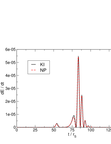
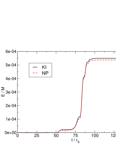
Figure 5: (Color online) Energy flux (left panel) and radiated energy (right panel) for the $l=2$ mode extracted at $R_{\rm ex}=50r_{S}$ from the KI wave function $\Phi_{,t}$ (black solid curve) and the Newman Penrose scalar $\Psi_{4}$ (red dashed curve).

We obtain an integrated energy of $5.5\times 10^{-4}~{}M$ and $5.3\times 10^{-4}~{}M$, respectively, for the gravitational wave energy radiated in $l=2$, where $M$ denotes the centre of mass energy.

The energy in the $l=2$ mode is known to contain more than $99\%$ of the total radiated energy Sperhake:2006cy . Our analysis is compatible with this finding; while the energy in the $l=3$ mode is zero by symmetry, our result for the energy in the $l=4$ mode obtained from the KI master function is three orders of magnitude smaller than that of the $l=2$ contribution.

IV Head-on collision from rest in $D=5$

Having tested the wave extraction formalism in four dimensions, we now turn our attention to the new results obtained for head-on collisions of BHs in five dimensional space-times. As before, we consider nonspinning BH binaries initially at rest with coordinate separation $d$. Note that in five space-time dimensions the Schwarzschild radius is related to the ADM mass $M$ via Eq. (8),

$$r_{S}^{2}=\frac{8M}{3\pi}\,.$$ (61)

We therefore define the “total” Schwarzschild radius $r_{S}$ such that $r_{S}^{2}=r_{S,1}^{2}+r_{S,2}^{2}$. By using this definition, $r_{S}$ has physical dimension of length and provides a suitable unit for measuring both, results and grid setup.

As summarized in Table 1, we consider a sequence of BH binaries with initial coordinate separation ranging from $d=3.17\,r_{S}$ to $d=10.37\,r_{S}$. The table further lists the proper separation $L$ along the line of sight between the holes and the grid configurations used for the individual simulations.

IV.1 Tests on the numerical coordinates

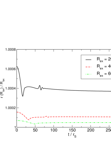
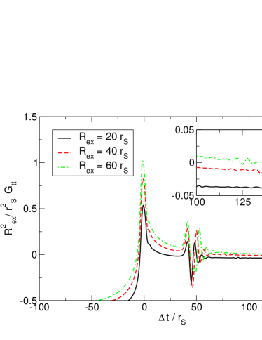
Figure 6: (Color online) Left panel: Time evolution of the areal radius $r$ in units of the extraction radius averaged over coordinate spheres at $R_{\rm ex}=20~{}r_{S}$ (black solid), $40~{}r_{S}$ (red dashed) and $60~{}r_{S}$ (green dash-dotted curve). Right panel: Deviation of the metric component $R_{\rm ex}^{2}/r_{S}^{2}\mathcal{G}_{tt}$ calculated from Eq. (16) at the same extraction radii and shifted in time to account for differences in the propagation time of the wave signal.

In order to verify the assumptions underlying our formalism, we have analysed the coordinate system in analogy to Sec. III.1. First, we have evaluated the averaged areal radius on extraction spheres of constant coordinate radius.

The result shown in the left panel of Fig. 6 demonstrates that the coordinate and areal radius agree within about 1 part in $10^{4}$ for $R_{\rm ex}\geq 40~{}r_{S}$. The Tangherlini coordinate $r$ equals by construction the areal radius and our approximation of setting $r\approx R_{\rm ex}$ in the wave extraction zone is satisfied with high precision.

Second, we evaluate the deviation of the metric components according to Eqs. (16)-(18). From the discussion in Sec. III.1 we expect $\mathcal{G}_{tt}\sim r^{2}/r_{S}^{2}$ in $D=5$. Our results in the right panel of Fig. 6 confirm this expectation and demonstrate that our space-time is indeed perturbatively close to that of a Tangherlini metric at sufficient distances from the black holes; deviations in $\mathcal{G}_{tt}$ are well below 1 part in $10^{3}$ at $R_{\rm ex}=60~{}r_{S}$. Furthermore, we can estimate the crudeness of the approximation $r^{2}_{S}=r^{2}_{S,1}+r^{2}_{S,2}$ for the Schwarzschild radius of the final BH: as shown in the right panel of Fig. 6, at late times $|R_{ex}^{2}/r_{S}^{2}\mathcal{G}_{tt}|\sim 0.01$; this value gives an upper bound on the radiated energy.

For the third test, we recall that our higher dimensional implementation does not employ the full isometry group of the $S^{2}$ sphere in $D=5$ dimensions and axial symmetry manifests itself instead in the conditions (20) on the metric components and the scalar field. We find these conditions to be satisfied within 1 part in $10^{8}$ and 1 part in $10^{16}$, respectively, in our numerical simulations which thus represent axially symmetric configurations with high precision.

IV.2 Newtonian collision time

An estimate of the time at which the holes “collide”, can be obtained by considering a Newtonian approximation to the kinematics of two point particles in $D=5$. In the weak-field regime, Einstein’s equations reduce to “Newton’s law” $a=-\nabla{\cal B}({\bf x})$, with $h_{00}=-2{\cal B}({\bf x})=r_{S}^{D-3}/2r^{D-3}$. The Newtonian time it takes for two point-masses (with Schwarzschild parameters $r_{S,1}$ and $r_{S,2}$) to collide from rest with initial distance $L$ in $D$ dimensions is then given by

$$\frac{t_{\text{free-fall}}}{r_{S}}=\frac{\mathcal{I}}{D-3}\left(\frac{L}{r_{S}}\right)^{\frac{D-1}{2}}\,,$$ (62)

where $r_{S}^{D-3}=r_{S,1}^{D-3}+r_{S,2}^{D-3}$ and

$$\mathcal{I}=\int_{0}^{1}\sqrt{\frac{z^{\frac{5-D}{D-3}}}{1-z}}dz=\sqrt{\pi}\frac{\Gamma(\frac{1}{2}+\frac{1}{D-3})}{\Gamma(1+\frac{1}{D-3})}\,.$$ (63)

For $D=4$, one recovers the standard result $t_{\text{free-fall}}=\pi\sqrt{L^{3}/r_{S}^{3}}r_{S}\,,$ whereas for $D=5$ we get

$$t_{\text{free-fall}}=\left(L/r_{S}\right)^{2}r_{S}\,.$$ (64)

In general relativity, BH trajectories and merger times are intrinsically observer dependent quantities. For our comparison with Newtonian estimates we have chosen relativistic trajectories as viewed by observers adapted to the numerical coordinate system. While the lack of fundamentally gauge invariant analogues in general relativity prevents us from deriving rigorous conclusions, we believe such a comparison to serve the intuitive interpretation of results obtained within the “moving puncture” gauge. Bearing in mind these caveats, we plot in Fig. 7 the analytical estimate of the Newtonian time of collision, together with the numerically computed time of formation of a common apparent horizon. Also shown in Fig. 7 is the time at which the separation between the individual hole’s puncture trajectory decreases below the Schwarzschild parameter $r_{S}$.

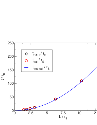
Figure 7: (Color online) Estimates for the time it takes for two equal-mass BHs to collide in $D=5$. The first estimate is given by the time $t_{\text{CAH}}$ elapsed until a single common apparent horizon engulfs both BHs (diamonds), the second estimate is obtained by using the trajectory of the BHs, i.e., the time $t_{\text{traj}}$ at which their separation has decreased below the Schwarzschild radius (circles). Finally, these numerical results are compared against a simple Newtonian estimate, given by Eq. (64) (blue solid line).

The remarkable agreement provides yet another example of how well numerically successful gauge conditions appear to be adapted to the black hole kinematics. It is beyond the scope of this paper to investigate whether this is coincidental or whether such agreement is necessary or at least helpful for gauge conditions to ensure numerical stability. Suffice it to say at this stage that similar conclusions were reached by Anninos et al. Anninos:1994gp and Lovelace et al. Lovelace:2009dg in similar four dimensional scenarios.

IV.3 Waveforms

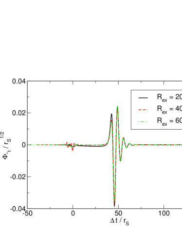
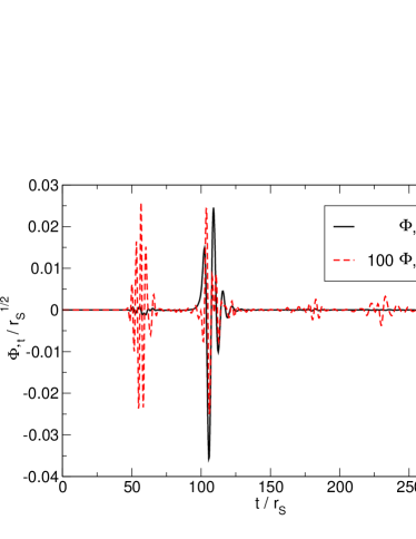
Figure 8: (Color online) Left panel: The $l=2$ component of the KI waveform for model HD5e_f extracted at radii $R_{\rm ex}/r_{S}=20,40$ and $60$ and shifted in time by $R_{\rm ex}/r_{S}$. Right panel: The $l=2$ and $l=4$ mode of the KI function for the same simulation, extracted at $R_{\rm ex}/r_{S}=60$. For clarity, the $l=4$ component has been re-scaled by a factor of $100$.

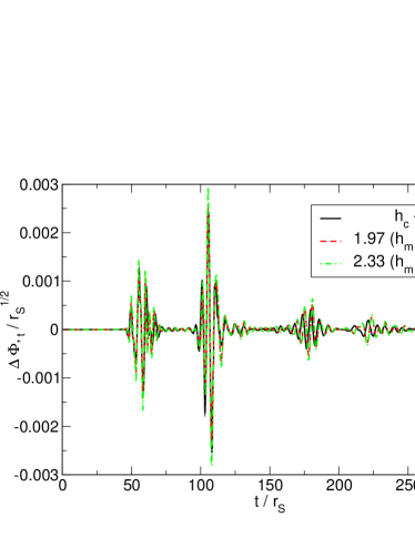
Figure 9: (Color online) Convergence analysis of the $l=2$ component of the KI function generated by model HD5e extracted at $R_{\rm ex}=60r_{S}$. The difference between the medium and high resolution waveforms has been amplified by the factors $1.97$ (red dashed line) and $2.33$ (green dashed-dotted line) indicating third and fourth order convergence.

We now discuss in detail the gravitational wave signal generated by the head-on collision of two BHs in five dimensions. For this purpose, we plot in Fig. 8 the $l=2$ multipole of the KI function $\Phi_{,t}$ for model HD5e_f obtained at different extraction radii. Qualitatively, the signal looks similar to that shown in the left panel of Fig. 2 for $D=4$. A small spurious wavepulse due to the initial data construction is visible at $\Delta t\approx 0$. This so-called “junk radiation” increases in magnitude if the simulation starts with smaller initial separation of the holes. We return to this issue further below, when we study the dependence of the gravitational radiation on the initial BH separation. The physical part of the waveform is dominated by the merger signal around $\Delta t=50~{}r_{S}$, followed by the (exponentially damped) ringdown, whereas the infall of the holes before $\Delta t=40~{}r_{S}$ does not produce a significant amount of gravitational waves. Comparison of the waveforms extracted at different radii demonstrates excellent agreement, in particular for those extracted at $R_{\rm ex}=40~{}r_{S}$ and $60~{}r_{S}$. Extrapolation of the radiated energy to infinite extraction radius yield a relative error of 5 % at $R_{\rm ex}=60~{}r_{S}$, indicating that such radii are adequate for the analysis presented in this work.

Due to symmetry, no gravitational waves are emitted in the $l=3$ multipole, so that $l=4$ represents the second strongest contribution to the wave signal. As demonstrated in the right panel of Fig. 2, however, its amplitude is two orders of magnitude below that of the quadrupole.

A convergence analysis also using the lower resolution simulations of models HD5e_c and HD5e_m is shown in Fig. 9 and demonstrates overall convergence of third to fourth order, consistent with the numerical implementation. From this analysis we obtain a conservative estimate of about $4\%$ for the discretization error in the waveform.

In practice, numerical simulations will always start with a finite separation of the two black holes. In order to assess how accurately we are thus able to approximate an infall from infinity, we have varied the initial separation for models HD5a to HD5f as summarized in Table 1. For small $d$ we observe two effects which make the physical interpretation of models HD5a$-$HD5c difficult. First, the amplitude of the spurious initial radiation increases and second, the shorter infall time causes an overlap of this spurious radiation with the merger signal. As demonstrated in Fig. 10 for models HD5e and HD5f, however, we can safely neglect the spurious radiation as well as the impact of a final initial separation, provided we use a sufficiently large initial distance $d\gtrsim 6~{}r_{S}$ of the BH binary. Here, we compare the radiation emitted during the head-on collision of BHs starting from rest with initial separations $6.37~{}r_{S}$ and $10.37~{}r_{S}$. The waveforms have been shifted in time by the extraction radius $R_{\rm ex}=60\,r_{S}$ and such that the formation of a common apparent horizon occurs at $\Delta t=0$. The merger signal starting around $\Delta t=0$ shows excellent agreement for the two configurations and is not affected by the spurious signal visible for HD5e at $\Delta t\approx-50~{}r_{S}$.

We conclude this discussion with two aspects of the post-merger part of the gravitational radiation, the ringdown and the possibility of GW tails. After formation of a common horizon, the waveform is dominated by an exponentially damped sinusoid, as the merged hole rings down into a stationary state. By fitting our results with a exponentially damped sinusoid, we obtain a characteristic frequency

$$r_{S}\,\omega=0.955\pm 0.005-{\rm i}\,(0.255\pm 0.005)\,.$$ (65)

This value is in excellent agreement with perturbative calculations, which predict a lowest quasinormal frequency $r_{S}\,\omega=0.9477-{\rm i}\,0.2561$ for $l=2$ Cardoso:2003qd ; Yoshino:2005ps ; Berti:2009kk .

A well known feature in gravitational waveforms generated in BH space-times with $D=4$ as well as $D>4$ are the so-called power-law tails DeWitt:1960fc ; Price:1971fb ; Ching:1995tj ; Cardoso:2003jf . In odd dimensional space-times an additional, different kind of late-time power tails arises, which does not depend on the presence of a BH. These are due to a peculiar behavior of the wave-propagation in flat odd dimensional space-times because the Green’s function has support inside the entire light-cone Cardoso:2003jf . We have attempted to identify such power-law tails in our signal at late-times, by subtracting a best-fit ringdown waveform. Unfortunately, we cannot, at this stage, report any evidence of such a power-law in our results, most likely because the low amplitude tails are buried in numerical noise.

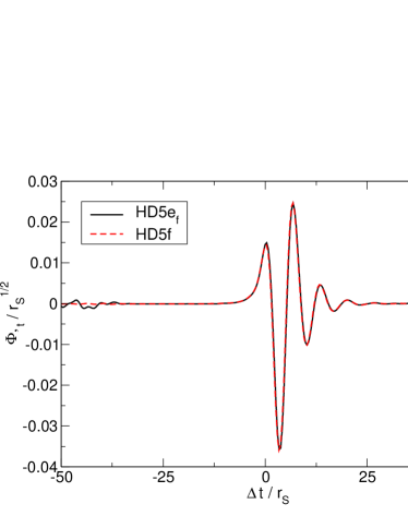
Figure 10: (Color online) The $l=2$ components of the KI function as generated by a head-on collision of BHs with initial (coordinate) distance $d=6.37\,r_{S}$ (black solid line) and $d=10.37\,r_{S}$ (red dashed line). The wave functions have been shifted in time such that the formation of a common apparent horizon corresponds to $\Delta t=0$ and taking into account the time it takes for the waves to propagate up to the extraction radius $R_{\rm ex}=60\,r_{S}$.

IV.4 Radiated energy

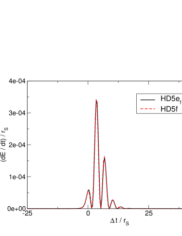
Figure 11: (Color online) Energy flux in the $l=2$ component of the KI wave function $\Phi_{,t}$, extracted at $R_{\rm ex}=60\,r_{S}$, for models HD5e_f (black solid line) and HD5f (red dashed line) in Table 1. The fluxes have been shifted in time by the extraction radius $R_{\rm ex}=60\,r_{S}$ and the time $t_{\text{CAH}}$ at which the common apparent horizon forms.

Comparison of Figs. 3 and 10 for the GW quadrupole in $D=4$ and $D=5$ shows a larger wave amplitude in the five dimensional case and thus indicates that this case may radiate more energy. We now investigate this question quantitatively by calculating the energy flux from the KI master function via Eq. (56). The fluxes thus obtained for the $l=2$ multipole of models HD5e_f and HD5f in Table 1, extracted at $R_{\rm ex}=60\,r_{S}$, are shown in Fig. 11. As in the case of the KI master function in Fig. 10, we see no significant variation of the flux for the two different initial separations. The flux reaches a maximum value of $dE/dt\sim 3.4\times 10^{-4}\,r_{S}$, and is then dominated by the ringdown flux. The energy flux from the $l=4$ mode is typically four orders of magnitude smaller; this is consistent with the factor of 100 difference of the corresponding wave multipoles observed in Fig. 8, and the quadratic dependence of the flux on the wave amplitude.

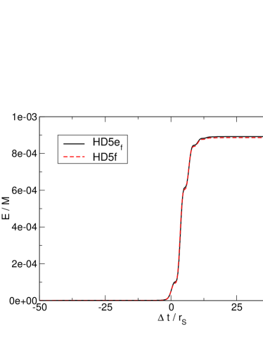
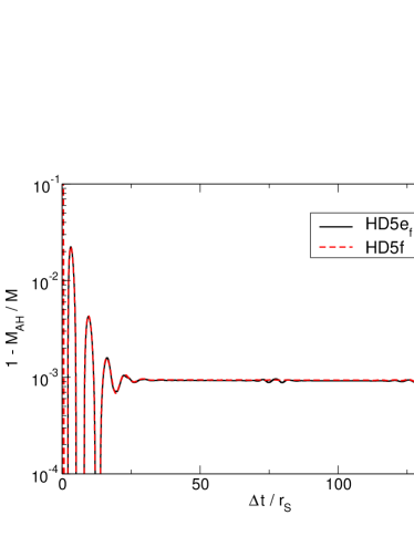
Figure 12: (Color online) Left panel: Fraction of the centre of mass energy, $E_{rad}/M$, radiated in the $l=2$ mode of the KI function shifted in time such that the origin of the time axis corresponds to the formation of a common apparent horizon. Right panel: Fraction of the centre of mass energy $1-M_{AH}/M$ radiated during the collision, estimated using apparent horizon information. The oscillations in this diagnostic quantity have a frequency comparable to the $l=2$ quasinormal mode frequency.

The total integrated energy emitted throughout the head-on collision is presented in the left panel of Fig. 12. We find that a fraction of $E_{rad}/M=(8.9\pm 0.6)\times 10^{-4}$ of the centre of mass energy is emitted in the form of gravitational radiation. We have verified for these models that the amount of energy contained in the spurious radiation is about three orders of magnitude smaller than in the physical merger signal.

An independent estimate for the radiated energy can be obtained from the apparent horizon area $A_{4}$ in the effective four dimensional space-time by using the spherical symmetry of the post-merger remnant hole. Energy balance then implies that the energy $E$ radiated in the form of GWs is given by

$$\frac{E}{M}=1-\frac{M_{AH}}{M}=1-\frac{A_{4}}{4\pi r_{S}^{2}}\,,$$ (66)

where $M_{AH}$ is the apparent horizon mass. The estimate $E/M$ is shown in Fig. 12 and reveals a behavior qualitatively similar to a damped sinusoid with constant offset. Indeed, by using a least square fit, we obtain a complex frequency $r_{S}\,\omega\sim 0.97-{i}\,0.29$, again similar to the fundamental $l=2$ quasinormal mode frequency (see discussion around Eq. (65)). At late times, $1-M_{AH}/M$ asymptotes to $1-M_{AH}/M\sim\left(9.3\pm 0.8\right)\times 10^{-4}$ which agrees very well with the GW estimate, within the numerical uncertainties.

V Discussion

In this paper we have developed a formalism to extract gravitational radiation observables from numerical simulations of head-on collisions of BHs in $D$ dimensions. Moreover, we have performed such simulations in $D=4,5$. The $D=4$ case serves as a test of our formalism and demonstrates consistency of our results with the literature. The $D=5$ case is entirely new. Besides obtaining the corresponding waveforms, we have shown that the total energy released in the form of gravitational waves is approximately $(0.089\pm 0.006)\%$ of the initial centre of mass energy of the system, for a head-on collision of two BHs starting from rest at very large distances. As a comparison, the analogous process in $D=4$ releases a slightly smaller quantity: $(0.055\pm 0.006)\%$. We summarize the main results for head-on collisions of two BHs starting from rest in four and five space-time dimensions in Table 2.

Table 2: Main results for head-on collisions in $D=4$ and $5$ dimensions. We list the ring down frequency $\omega$, the total energy radiated in gravitational waves, the upper bound $E^{\rm area}$ on the radiated energy obtained from Hawking’s area theorem and the fractional energy in the $l=4$ multipole relative to the quadrupole radiation.

$D$	$r_{S}\,\omega(l=2)$	$E^{\rm rad}/M(\%)$	$E^{\rm area}/M(\%)$	$E^{\rm rad}_{l=4}/E^{\rm rad}_{l=2}$
$4$	$0.7473-{\rm i}\,0.1779$	$0.055$	$29.3$	$<10^{-3}$
$5$	$0.9477-{\rm i}\,0.2561$	$0.089$	$20.6$	$<10^{-4}$

We have further performed a variety of tests of the wave extraction formalism. Besides testing the proximity of the numerical coordinate system to the Tangherlini background space-time, we have demonstrated good agreement between the radiated energy as derived directly from the KI master function with the values obtained from the horizon area of the post-merger remnant hole. Finally, the ringdown part of the waveform yields a quasinormal mode frequency in excellent agreement with predictions from BH perturbation theory.

The radiative efficiency $E^{\rm rad}/M$ in Table 2 shows that head-on collisions starting from rest in five dimensions generate about 1.6 times as much GW energy as their four dimensional counterparts. It will be very interesting to investigate to what extent this observation holds for wider classes of BH collisions. We can compare the radiation efficiency with the upper limit derived by Hawking Hawking:1971 from the requirement that the horizon area must not decrease in the collision. This leads to the area bound $\frac{E^{\rm area}}{M}\leq 1-2^{-\frac{1}{D-2}}\,.$ Evidently, this bound decreases with dimensionality, while in the present computation it increases when going from $D=4$ to $D=5$. As also shown in the table, the generation of GWs in head-on collisions starting from rest is about 3 orders of magnitude below this bound. In four dimensions it has already been demonstrated that there exist more violent processes which release more radiation than the head-on collisions considered in this work Sperhake:2008ga ; Shibata:2008rq ; Sperhake:2009jz .

In the context of this work, it would be particularly interesting to compute the gravitational radiation emitted when a point particle falls into a higher dimensional BH (the four dimensional calculation is done in the classic work by Davis et al Davis:1971gg ). This analysis can be done by linearizing Einstein’s equations. While such an analysis was done for infall at high energies Cardoso:2002ay ; Berti:2003si , it has not been done for infalls from rest. The four dimensional case shows that by scaling the point-particle results properly with the reduced mass, one gets surprisingly good agreement with full nonlinear studies Anninos:1993zj . An obvious question is whether such an agreement extends to generic number of space-time dimensions. Investigations with a similar purpose, but using a different technique, were carried out in Refs. Araujo:1995vb ; Moreschi:1996ds .

The numbers reported here for the total energy loss in gravitational waves should increase significantly in high energy collisions, which are the most relevant scenarios for the applications described in the Introduction. Indeed, in the four dimensional case, it is known that ultra-relativistic head-on collisions of equal mass nonrotating BHs release up to 14% of the initial centre of mass energy into gravitational radiation Sperhake:2008ga . The analogous number in higher dimensions is as yet unknown and will be subject of the next stages of our research programme. Preliminary results by Gal’tsov et al Gal'tsov:2009zi ; Gal'tsov:2010me strongly suggest enhancement of radiation emission for higher dimensions, in agreement with the $D=5$ results shown here. Even more energy may be released in high energy collisions with nonvanishing impact parameter. In Shibata:2008rq ; Sperhake:2009jz it was shown that this number can be as large as 35% in $D=4$. The formalism developed in Paper I allows, in principle, the study of analogous processes in $D\geq 6$. We hope to be able to report on these results in the near future.

Appendix A Coordinate transformation

In order to extract gravitational radiation using the KI formalism one has to perform a coordinate transformation from Cartesian coordinates, which are used during the numerical evolution, to those adapted for wave extraction. The physical 3-metric $\gamma_{ij}$, the lapse function $\alpha$ and the shift vector $\beta^{i}$ computed on our Cartesian grid are interpolated onto a Cartesian patch. In terms of these quantities we compute the 4-metric $g_{\mu\nu}$ in Cartesian coordinates according to Eq. (2):

$$g_{\mu\nu}dx^{\mu}dx^{\nu}= (-\alpha^{2}+\gamma_{ij}\beta^{i}\beta^{j})dt^{2}+\gamma_{ij}\beta^{i}dtdx^{j}$$

$$+\gamma_{ij}\beta^{j}dtdx^{i}+\gamma_{ij}dx^{i}dx^{j}\,.$$ (67)

Then, we transform the 4-metric in Cartesian coordinates into spherical coordinates, defined by Eq. (12)

$$x =R\sin\bar{\theta}\cos\theta\,,$$ (68)

$$y =R\sin\bar{\theta}\sin\theta\,,$$ (69)

$$z =R\cos\bar{\theta}\,,$$ (70)

where $\bar{\theta},\theta\in[0,\pi]$ and $R=\sqrt{x^{2}+y^{2}+z^{2}}$. If we denote the metric in spherical coordinates by $g_{\mu\nu}^{S}$ and define $\rho\equiv\sqrt{x^{2}+y^{2}}$, the explicit form of the transformation is

$$g^{S}_{tR}= g_{tx}\sin\bar{\theta}\cos\theta+g_{ty}\sin\bar{\theta}\sin\theta+g_{tz}\cos\bar{\theta}\,,$$ (71)

$$g^{S}_{t\bar{\theta}}= z(g_{tx}\cos\theta+g_{ty}\sin\theta)-\rho g_{tz}\,,$$ (72)

$$g^{S}_{t\theta}= -yg_{tx}+xg_{ty}\,,$$ (73)

$$g^{S}_{RR}= g_{xx}\sin^{2}\bar{\theta}\cos^{2}\theta+2g_{xy}\sin^{2}\bar{\theta}\cos\theta\sin\theta$$

$$+2g_{xz}\sin\bar{\theta}\cos\theta\cos\bar{\theta}+g_{yy}\sin^{2}\bar{\theta}\sin^{2}\theta$$

$$+2g_{yz}\sin\bar{\theta}\sin\theta\cos\bar{\theta}+g_{zz}\cos^{2}\bar{\theta}\,,$$ (74)

$$g^{S}_{R\bar{\theta}}= z(g_{xx}\sin\bar{\theta}\cos^{2}\theta+2g_{xy}\sin\bar{\theta}\cos\theta\sin\theta$$

$$+g_{yy}\sin\bar{\theta}\sin^{2}\theta+g_{xz}\cos\bar{\theta}\cos\theta+g_{yz}\cos\bar{\theta}\sin\theta)$$

$$-(xg_{xz}+yg_{yz}+zg_{zz})\sin\bar{\theta}\,,$$ (75)

$$g^{S}_{R\theta}= (-yg_{xx}\sin\bar{\theta}\cos\theta+xg_{xy}\sin\bar{\theta}\cos\theta-yg_{xy}\sin\bar{\theta}\sin\theta$$

$$+xg_{yy}\sin\bar{\theta}\sin\theta-yg_{xz}\cos\bar{\theta}+xg_{yz}\cos\bar{\theta})\,,$$ (76)

$$g^{S}_{\bar{\theta}\bar{\theta}}= z^{2}(g_{xx}\cos^{2}\theta+2g_{xy}\cos\theta\sin\theta+g_{yy}\sin^{2}\theta)$$

$$-2z(xg_{xz}+yg_{yz})+\rho^{2}g_{zz}\,,$$ (77)

$$g^{S}_{\bar{\theta}\theta}= z(-yg_{xx}\cos\theta+xg_{xy}\cos\theta-yg_{xy}\sin\theta$$

$$+xg_{yy}\sin\theta)+\rho(yg_{xz}-xg_{yz})\,,$$ (78)

$$g^{S}_{\theta\theta}= R^{2}\sin^{2}\bar{\theta}(g_{xx}\sin^{2}\theta-2g_{xy}\cos\theta\sin\theta+g_{yy}\cos^{2}\theta)\,.$$ (79)

Henceforth, we will drop the superscript $S$ and use $g_{\mu\nu}$ for the metric in spherical coordinates.

The areal radius $r$ is related to $R$ by a reparametrization $R=R(r)$, given by Eq. (127), which depends on the components $g_{\bar{\theta}\bar{\theta}}$, $g_{\theta\theta}$ only. As shown in Section III, we find that this reparametrization is nearly constant throughout our numerical simulations. Therefore, the quantities $g_{rr},g_{tr}$, $g_{r\bar{\theta}},g_{r\theta}$ can be obtained from $g_{RR},g_{tR},g_{R\bar{\theta}},g_{R\theta}$ by a simple rescaling: because

$$\frac{dR}{dr}\simeq 1\,,$$ (80)

we have $g_{rr}\simeq g_{RR}$, and similar relations hold for the other components.

Appendix B Harmonic expansion of axisymmetric tensors in $D$ dimensions

As discussed in Section II.3, scalar spherical harmonics in $D$ dimensions ${\cal S}_{l}(\bar{\theta},\theta,\phi^{1},\dots,\phi^{D-4})$ are solutions of Eq. (23)

$$\Box{\cal S}_{l}=\gamma^{\bar{i}\bar{j}}{\cal S}_{l\,:\bar{i}\bar{j}}=-k^{2}{\cal S}_{l}\,,$$ (81)

with $k^{2}=l(l+D-3)$. Axisymmetric scalar spherical harmonics are functions of the coordinate $\bar{\theta}$ only, ${\cal S}_{l}={\cal S}_{l}(\bar{\theta})$. Therefore, Eq. (81) becomes

$$\Box{\cal S}_{l}(\bar{\theta})={\cal S}_{l\,,\bar{\theta}\bar{\theta}}+(D-3)\cot\bar{\theta}{\cal S}_{l\,,\bar{\theta}}=-k^{2}{\cal S}_{l}\,,$$ (82)

since

$${\cal S}_{l\,:\bar{\theta}\bar{\theta}} ={\cal S}_{l\,,\bar{\theta}\bar{\theta}}\,$$ (83)

$${\cal S}_{l\,:\theta\theta} =-\Gamma_{\theta\theta}^{\bar{\theta}}{\cal S}_{l\,,\bar{\theta}}=\sin\bar{\theta}\cos\bar{\theta}{\cal S}_{l\,,\bar{\theta}}\,,$$ (84)

$${\cal S}_{l\,:\phi^{1}\phi^{1}} =-\Gamma_{\phi^{1}\phi^{1}}^{\bar{\theta}}{\cal S}_{l\,,\bar{\theta}}=\sin^{2}\theta\sin\bar{\theta}\cos\bar{\theta}{\cal S}_{l\,,\bar{\theta}}\,,$$ (85)

etc. The quantities ${\cal S}_{l\,\bar{i}\bar{j}}$ defined in Eq. (24) are then

$${\cal S}_{l\,\bar{i}\bar{j}}= \frac{1}{k^{2}}{\cal S}_{l\,:\bar{i}\bar{j}}+\frac{1}{D-2}\gamma_{\bar{i}\bar{j}}{\cal S}_{l}$$

$$= \frac{1}{k^{2}(D-2)}\left((D-2){\cal S}_{l\,:\bar{i}\bar{j}}+k^{2}\gamma_{\bar{i}\bar{j}}{\cal S}_{l}\right)$$

$$= \frac{1}{k^{2}(D-2)}{\rm diag}\left((D-3){\cal W}_{l},\right.$$

$$\left.-\sin^{2}\bar{\theta}{\cal W}_{l},-\sin^{2}\bar{\theta}\sin^{2}\theta{\cal W}_{l},\dots\right)$$ (86)

where

$${\cal W}_{l}(\bar{\theta})={\cal S}_{l\,,\bar{\theta}\bar{\theta}}-\cot\bar{\theta}{\cal S}_{l\,,\bar{\theta}}=\sin\bar{\theta}\left(\frac{{\cal S}_{l\,,\bar{\theta}}}{\sin\bar{\theta}}\right)_{,\bar{\theta}}\,.$$ (87)

Indeed, using Eq. (82) one finds

$$k^{2}(D-2){\cal S}_{l\,\bar{\theta}\bar{\theta}}= (D-2){\cal S}_{l\,,\bar{\theta}\bar{\theta}}+k^{2}{\cal S}_{l}$$

$$= (D-3)({\cal S}_{l\,,\bar{\theta}\bar{\theta}}-\cot\bar{\theta}{\cal S}_{l\,,\bar{\theta}})\,,$$ (88)

$$k^{2}(D-2){\cal S}_{l\,\theta\theta} =(D-2){\cal S}_{l\,,\theta\theta}+k^{2}\sin^{2}\bar{\theta}{\cal S}_{l}$$

$$= \sin^{2}\bar{\theta}((D-2)\cot\bar{\theta}{\cal S}_{l\,,\bar{\theta}}+k^{2}{\cal S}_{l})$$

$$= \sin^{2}\bar{\theta}(-{\cal S}_{l\,,\bar{\theta}\bar{\theta}}+\cot\bar{\theta}{\cal S}_{l\,,\bar{\theta}})\,,$$ (89)

and therefore

$${\cal S}_{l\,\bar{\theta}\bar{\theta}}= \frac{D-3}{k^{2}(D-2)}{\cal W}_{l}\,,$$ (90)

$${\cal S}_{l\,\theta\theta}= -\frac{\sin^{2}\bar{\theta}}{k^{2}(D-2)}{\cal W}_{l}\,,$$ (91)

and likewise for the other components.

Axisymmetric scalar spherical harmonics, as discussed in Sec. II.3, can be written in terms of Gegenbauer polynomials (cf. (37)):

$${\cal S}_{l}(\bar{\theta})=(K^{lD})^{-1/2}C_{l}^{(D-3)/2}(\cos\bar{\theta})\,.$$ (92)

If we define

$$W_{l}(\cos\bar{\theta})=C_{l\,,\bar{\theta}\bar{\theta}}^{(D-3)/2}(\cos\bar{\theta})-\cot\bar{\theta}C_{l\,,\bar{\theta}}^{(D-3)/2}(\cos\bar{\theta})\,,$$ (93)

we have

$${\cal W}_{l}(\bar{\theta})=(K^{lD})^{-1/2}W_{l}^{(D-3)/2}(\cos\bar{\theta})\,.$$ (94)

We impose the normalization (38)

$$\int d\Omega^{D-2}{\cal S}_{l}{\cal S}_{l^{\prime}}=\delta_{ll^{\prime}}\,,~{}~{}~{}\int d\Omega^{D-2}{\cal S}_{l\,,\bar{\theta}}{\cal S}_{l^{\prime}\,,\bar{\theta}}=\delta_{ll^{\prime}}k^{2}\,.$$ (95)

Using

$$\int_{0}^{\pi}d\bar{\theta}(\sin\bar{\theta})^{D-3}C_{l}^{(D-3)/2}(\cos{\bar{\theta}})C_{l^{\prime}}^{(D-3)/2}(\cos{\bar{\theta}})= \delta_{ll^{\prime}}\hat{K}^{lD}\,,$$ (96)

$$\int_{0}^{\pi}d\bar{\theta}(\sin\bar{\theta})^{D-3}C_{l\,,\bar{\theta}}^{(D-3)/2}(\cos{\bar{\theta}})C_{l^{\prime}\,,\bar{\theta}}^{(D-3)/2}(\cos{\bar{\theta}})$$

$$=\delta_{ll^{\prime}}k^{2}\hat{K}^{lD} \,,$$ (97)

and

$$\hat{K}^{lD}=\frac{2^{4-D}\pi\Gamma(l+D-3)}{\left(l+\frac{D-3}{2}\right)\left(\Gamma\left(\frac{D-3}{2}\right)\right)^{2}\Gamma(l+1)}\,,$$ (98)

we have

$$K^{lD}=\hat{K}^{lD}{\cal A}_{D-3}\,,$$ (99)

where

$${\cal A}_{D-3}=\frac{2\pi^{(D-2)/2}}{\Gamma\left(\frac{D-2}{2}\right)}\,,$$ (100)

is the surface of the $(D-3)$-sphere $S^{D-3}$. Note that $\int d\Omega^{D-2}(\cdots)={\cal A}_{D-3}\int d\bar{\theta}(\sin\bar{\theta})^{D-3}(\cdots)$. With the definitions (24) ${\cal S}_{l\,\bar{i}}=-\frac{1}{k}{\cal S}_{l\,,\bar{i}}$,

$$\int_{0}^{\pi}d\tilde{\theta}(\sin\bar{\theta})^{D-3}{\cal S}_{l}(\tilde{\theta}){\cal S}_{l^{\prime}}(\bar{\theta})= \delta_{ll^{\prime}}{\cal A}_{D-3}^{-1}\,,$$ (101)

$$\int_{0}^{\pi}d\tilde{\theta}(\sin\tilde{\theta})^{D-3}\gamma^{\bar{i}\bar{j}}{\cal S}_{l\,\bar{i}}{\cal S}_{l^{\prime}\,\bar{j}}$$

$$=\int_{0}^{\pi}d\tilde{\theta}(\sin\tilde{\theta})^{D-3}{\cal S}_{l\,\bar{\theta}}(\bar{\theta}){\cal S}_{l^{\prime}\,\bar{\theta}}(\bar{\theta})$$

$$=\delta_{ll^{\prime}}{\cal A}_{D-3}^{-1}\,.$$ (102)

Furthermore, we note that Eqs. (82) and (87) imply

$${\cal W}_{l}+(D-2)\cot\bar{\theta}{\cal S}_{l\,,\bar{\theta}}+k^{2}{\cal S}_{l}=0\,,$$ (103)

so that

$${\cal W}_{l\,,\bar{\theta}}+(D-2)\cot\bar{\theta}{\cal S}_{l\,,\bar{\theta}\bar{\theta}}-\frac{D-2}{\sin^{2}\bar{\theta}}{\cal S}_{l\,,\bar{\theta}}+k^{2}{\cal S}_{l\,,\bar{\theta}}$$

$$={\cal W}_{l\,,\bar{\theta}}+(D-2)\cot\bar{\theta}{\cal W}_{l}+(k^{2}-D+2){\cal S}_{l\,,\bar{\theta}}\,,$$ (104)

and therefore

$$\int_{0}^{\pi}d\bar{\theta}(\sin\bar{\theta})^{D-3}{\cal W}_{l}{\cal W}_{l^{\prime}}$$

$$= \int_{0}^{\pi}d\bar{\theta}(\sin\bar{\theta})^{D-3}{\cal W}_{l}\sin\bar{\theta}\left(\frac{{\cal S}_{l^{\prime}\,,\bar{\theta}}}{\sin\bar{\theta}}\right)_{,\bar{\theta}}$$

$$= -(D-2)\int_{0}^{\pi}d\bar{\theta}(\sin\bar{\theta})^{D-3}{\cal W}_{l}\cot\bar{\theta}{\cal S}_{l^{\prime}\,,\bar{\theta}}$$

$$-\int_{0}^{\pi}d\bar{\theta}(\sin\bar{\theta})^{D-3}{\cal W}_{l\,,\bar{\theta}}{\cal S}_{l^{\prime}\,,\bar{\theta}}$$

$$= (k^{2}-D+2)\int_{0}^{\pi}d\bar{\theta}(\sin\bar{\theta})^{D-3}{\cal S}_{l\,,\bar{\theta}}{\cal S}_{l^{\prime}\,,\bar{\theta}}$$

$$= \delta_{ll^{\prime}}{\cal A}_{D-3}^{-1}\,k^{2}(k^{2}-D+2)\,.$$ (105)

We thus obtain

$$\int d\Omega^{D-2}{\cal W}_{l}{\cal W}_{l^{\prime}}=\delta_{ll^{\prime}}k^{2}(k^{2}-D+2)\,.$$ (106)

The perturbations $f^{l}_{ab}(t,r)$, $f^{l}_{a}(t,r)$, $H^{l}_{L}(t,r)$, $H^{l}_{T}(t,r)$ appearing in the expansion of the metric perturbations (II.3)

$$h_{ab} =f^{l}_{ab}{\cal S}_{l}(\bar{\theta})\,,$$ (107)

$$h_{a\bar{\theta}} =-\frac{1}{k}rf^{l}_{a}{\cal S}_{l}(\bar{\theta})_{,\bar{\theta}}\,,$$ (108)

$$h_{\bar{\theta}\bar{\theta}} =2r^{2}\left(H^{l}_{L}{\cal S}_{l}(\bar{\theta})+H^{l}_{T}\frac{D-3}{k^{2}(D-2)}{\cal W}_{l}(\bar{\theta})\right)\,,$$ (109)

$$h_{\theta\theta} =2r^{2}\sin^{2}\bar{\theta}\left(H^{l}_{L}{\cal S}_{l}(\bar{\theta})-H^{l}_{T}\frac{1}{k^{2}(D-2)}{\cal W}_{l}(\bar{\theta})\right)\,.$$ (110)

are given by the following integrals, as follows from Eqs. (92), (94), (95), (106):

$$f^{l}_{ab}(t,r)= \int d\Omega^{D-2}h_{ab}{\cal S}_{l}$$

$$= \frac{{\cal A}_{D-3}}{\sqrt{K^{lD}}}\int_{0}^{\pi}d\bar{\theta}(\sin\bar{\theta})^{D-3}h_{ab}C_{l}^{(D-3)/2}\,,$$ (111)

$$f_{a}(t,r)= -\frac{1}{kr}\int d\Omega^{D-2}h_{a\bar{\theta}}{\cal S}_{l\,,\bar{\theta}}$$

$$= -\frac{1}{kr}\frac{{\cal A}_{D-3}}{\sqrt{K^{lD}}}\int_{0}^{\pi}d\bar{\theta}(\sin\bar{\theta})^{D-3}h_{a\bar{\theta}}C_{l\,,\bar{\theta}}^{(D-3)/2}\,,$$ (112)

$$H_{L}(t,r)= \frac{1}{2(D-2)r^{2}}\int d\Omega^{D-2}\left[h_{\bar{\theta}\bar{\theta}}+\frac{D-3}{\sin^{2}\bar{\theta}}h_{\theta\theta}\right]{\cal S}_{l}$$

$$= \frac{1}{2(D-2)r^{2}}\frac{{\cal A}_{D-3}}{\sqrt{K^{lD}}}\int_{0}^{\pi}d\bar{\theta}(\sin\bar{\theta})^{D-3}$$

$$\times\left[h_{\bar{\theta}\bar{\theta}}+\frac{D-3}{\sin^{2}\bar{\theta}}h_{\theta\theta}\right]C_{l}^{(D-3)/2}\,,$$ (113)

$$H_{T}(t,r)= \frac{1}{2r^{2}(k^{2}-D+2)}\int d\Omega^{D-2}$$

$$\times\left[h_{\bar{\theta}\bar{\theta}}-\frac{1}{\sin^{2}\bar{\theta}}h_{\theta\theta}\right]{\cal W}_{l}$$

$$= \frac{1}{2r^{2}(k^{2}-D+2)}\frac{{\cal A}_{D-3}}{\sqrt{K^{lD}}}\int_{0}^{\pi}d\bar{\theta}(\sin\bar{\theta})^{D-3}$$

$$\times\left[h_{\bar{\theta}\bar{\theta}}-\frac{1}{\sin^{2}\bar{\theta}}h_{\theta\theta}\right]W_{l}\,,$$ (114)

where $h_{ab}=h_{ab}(t,r,\bar{\theta})$, $h_{a\bar{\theta}}=h_{a\bar{\theta}}(t,r,\bar{\theta})$, $h_{\bar{\theta}\bar{\theta}}=h_{\bar{\theta}\bar{\theta}}(t,r,\bar{\theta})$, $h_{\theta\theta}=h_{\theta\theta}(t,r,\bar{\theta})$, $C_{l}^{(D-3)/2}=C_{l}^{(D-3)/2}(\cos{\bar{\theta}})$ and $W_{l}=W_{l}(\cos\bar{\theta})$.

We also note that the background Tangherlini metric depends on the $l=0$ harmonic only; the integral of its components over $l\geq 2$ harmonics vanish. Therefore, if we decompose the space-time metric (see Appendix A) as $g_{\mu\nu}=g^{(0)}_{\mu\nu}+h_{\mu\nu}$ with $\mu,\nu=(t,r,\bar{\theta},\theta)$ and $g^{(0)}_{\mu\nu}$ is the Tangherlini background metric, we can compute the integrals (114) in terms of the metric $g_{\mu\nu}$

$$f_{tt}= \frac{1}{\pi}\frac{{\cal A}_{D-3}}{\sqrt{K^{lD}}}\int d\bar{\theta}(\sin\bar{\theta})^{D-3}C_{l}^{(D-3)/2}\int d\theta g_{tt}(\bar{\theta},\theta)\,,$$ (115)

$$f_{tr}= \frac{1}{\pi}\frac{{\cal A}_{D-3}}{\sqrt{K^{lD}}}\int d\bar{\theta}(\sin\bar{\theta})^{D-3}C_{l}^{(D-3)/2}\int d\theta g_{tr}(\bar{\theta},\theta)\,,$$ (116)

$$f_{rr}= \frac{1}{\pi}\frac{{\cal A}_{D-3}}{\sqrt{K^{lD}}}\int d\bar{\theta}(\sin\bar{\theta})^{D-3}C_{l}^{(D-3)/2}\int d\theta g_{rr}(\bar{\theta},\theta)\,,$$ (117)

$$f_{t}= -\frac{1}{kr\pi}\frac{{\cal A}_{D-3}}{\sqrt{K^{lD}}}$$

$$\times\int d\bar{\theta}(\sin\bar{\theta})^{D-3}\partial_{\bar{\theta}}C_{l}^{(D-3)/2}\int d\theta g_{t\bar{\theta}}(\bar{\theta},\theta)\,,$$ (118)

$$f_{r}= -\frac{1}{kr\pi}\frac{{\cal A}_{D-3}}{\sqrt{K^{lD}}}$$

$$\times\int d\bar{\theta}(\sin\bar{\theta})^{D-3}\partial_{\bar{\theta}}C_{l}^{(D-3)/2}\int d\theta g_{r\bar{\theta}}(\bar{\theta},\theta)\,,$$ (119)

$$H_{L}= \frac{1}{2(D-2)r^{2}\pi}\frac{{\cal A}_{D-3}}{\sqrt{K^{lD}}}\int d\bar{\theta}(\sin\bar{\theta})^{D-3}C_{l}^{(D-3)/2}$$

$$\times\int d\theta\left(g_{\bar{\theta}\bar{\theta}}(\bar{\theta},\theta)+(D-3)\frac{g_{\theta\theta}(\bar{\theta},\theta)}{\sin^{2}\bar{\theta}}\right)\,,$$ (120)

$$H_{T}= \frac{1}{2(k^{2}-D+2)r^{2}\pi}\frac{{\cal A}_{D-3}}{\sqrt{K^{lD}}}$$

$$\times\int d\bar{\theta}(\sin\bar{\theta})^{D-3}W_{l}\int d\theta\left(g_{\bar{\theta}\bar{\theta}}(\bar{\theta},\theta)-\frac{g_{\theta\theta}(\bar{\theta},\theta)}{\sin^{2}\bar{\theta}}\right)\,.$$ (121)

Furthermore, from Eqs. (• ‣ II.2) and (115) - (B) we deduce

$$F_{,t}= \partial_{t}H_{L}+\frac{1}{D-2}\partial_{t}H_{T}+\frac{1}{k}f(r)\left(\partial_{t}f_{r}+\frac{r}{k}\partial_{t}\partial_{r}H_{T}\right)\,,$$ (122)

$$F^{r}_{t}= f(r)\left(f_{rt}+\frac{r}{k}(\partial_{t}f_{r}+\partial_{r}f_{t})+\frac{1}{k}f_{t}\right.$$

$$\left.+\frac{2r}{k^{2}}(\partial_{t}H_{T}+r\partial_{t}\partial_{r}H_{T})\right)-\frac{r}{k}\partial_{r}f(r)\left(f_{t}+\frac{r}{k}\partial_{t}H_{T}\right)\,.$$ (123)

Conversely, since the perturbations do not depend on the $l=0$ harmonic, the background metric $g_{\mu\nu}$ can be obtained as follows:

$$g_{tt}^{(0)} =\frac{1}{K^{0D}\pi}\int_{0}^{\pi}d\bar{\theta}\sin^{D-3}\bar{\theta}\int_{0}^{\pi}d\theta g_{tt}(\bar{\theta},\theta)\,,$$ (124)

$$g_{tr}^{(0)} =0=\frac{1}{K^{0D}\pi}\int_{0}^{\pi}d\bar{\theta}\sin^{D-3}\bar{\theta}\int_{0}^{\pi}d\theta g_{tr}(\bar{\theta},\theta)\,,$$ (125)

$$g_{rr}^{(0)} =\frac{1}{K^{0D}\pi}\int_{0}^{\pi}d\bar{\theta}\sin^{D-3}\bar{\theta}\int_{0}^{\pi}d\theta g_{rr}(\bar{\theta},\theta)\,.$$ (126)

Finally, to compute the areal radius $r$ we note that $g_{\bar{\theta}\bar{\theta}}=r^{2}+h_{\bar{\theta}\bar{\theta}}$ and $g_{\theta\theta}=r^{2}\sin^{2}\bar{\theta}+h_{\theta\theta}$. Both the perturbations $h_{\bar{\theta}\bar{\theta}}$ and $h_{\theta\theta}$ contain harmonics of different type (${\cal S}_{l}$, ${\cal S}_{l\,,\bar{i}\bar{j}}$); to extract the background we need the combination in Eq. (B):

$$r^{2}= \frac{1}{(D-2)K^{0D}\pi}\int_{0}^{\pi}d\bar{\theta}\sin^{D-3}\bar{\theta}\int_{0}^{\pi}d\theta$$

$$\times\left[g_{\bar{\theta}\bar{\theta}}+(D-3)\frac{g_{\theta\theta}}{\sin^{2}\bar{\theta}}\right]\,.$$ (127)

References

- (1) M. Zilhao et al., Phys. Rev. D81, 084052 (2010), [1001.2302].
- (2) R. Emparan and H. S. Reall, Living Rev. Rel. 11, 6 (2008), [0801.3471].
- (3) J. M. Maldacena, Adv. Theor. Math. Phys. 2, 231 (1998), [hep-th/9711200].
- (4) I. Antoniadis, Phys. Lett. B246, 377 (1990).
- (5) N. Arkani-Hamed, S. Dimopoulos and G. R. Dvali, Phys. Lett. B429, 263 (1998), [hep-ph/9803315].
- (6) I. Antoniadis, N. Arkani-Hamed, S. Dimopoulos and G. R. Dvali, Phys. Lett. B436, 257 (1998), [hep-ph/9804398].
- (7) L. Randall and R. Sundrum, Phys. Rev. Lett. 83, 3370 (1999), [hep-ph/9905221].
- (8) L. Randall and R. Sundrum, Phys. Rev. Lett. 83, 4690 (1999), [hep-th/9906064].
- (9) F. Pretorius, 0710.1338.
- (10) I. Hinder, Class. Quant. Grav. 27, 114004 (2010), [1001.5161].
- (11) M. Shibata and H. Yoshino, Phys. Rev. D81, 021501 (2010), [0912.3606].
- (12) M. Shibata and H. Yoshino, Phys. Rev. D81, 104035 (2010), [1004.4970].
- (13) H. Yoshino and M. Shibata, Phys. Rev. D80, 084025 (2009), [0907.2760].
- (14) H. Witek et al., Phys. Rev. D82, 104037 (2010), [1004.4633].
- (15) T. Banks and W. Fischler, hep-th/9906038.
- (16) S. B. Giddings and S. D. Thomas, Phys. Rev. D65, 056010 (2002), [hep-ph/0106219].
- (17) S. Dimopoulos and G. L. Landsberg, Phys. Rev. Lett. 87, 161602 (2001), [hep-ph/0106295].
- (18) J. L. Feng and A. D. Shapere, Phys. Rev. Lett. 88, 021303 (2001), [hep-ph/0109106].
- (19) E.-J. Ahn, M. Ave, M. Cavaglia and A. V. Olinto, Phys. Rev. D68, 043004 (2003), [hep-ph/0306008].
- (20) E.-J. Ahn, M. Cavaglia and A. V. Olinto, Phys. Lett. B551, 1 (2003), [hep-th/0201042].
- (21) A. Chamblin, F. Cooper and G. C. Nayak, Phys. Rev. D70, 075018 (2004), [hep-ph/0405054].
- (22) V. Cardoso, M. C. Espirito Santo, M. Paulos, M. Pimenta and B. Tome, Astropart. Phys. 22, 399 (2005), [hep-ph/0405056].
- (23) M. Cavaglia, Int. J. Mod. Phys. A18, 1843 (2003), [hep-ph/0210296].
- (24) P. Kanti, Int. J. Mod. Phys. A19, 4899 (2004), [hep-ph/0402168].
- (25) P. Kanti, Lect. Notes Phys. 769, 387 (2009), [0802.2218].
- (26) S. N. Solodukhin, Phys. Lett. B533, 153 (2002), [hep-ph/0201248].
- (27) S. D. H. Hsu, Phys. Lett. B555, 92 (2003), [hep-ph/0203154].
- (28) K. S. Thorne, In Magic Without Magic, edited by J. Klauder (W.H. Freeman & co., San Francisco, 1972), 231-258.
- (29) M. W. Choptuik and F. Pretorius, Phys. Rev. Lett. 104, 111101 (2010), [0908.1780].
- (30) M. Cavaglia, R. Godang, L. Cremaldi and D. Summers, Comput. Phys. Commun. 177, 506 (2007), [hep-ph/0609001].
- (31) J. A. Frost et al., JHEP 10, 014 (2009), [0904.0979].
- (32) D.-C. Dai et al., Phys. Rev. D77, 076007 (2008), [0711.3012].
- (33) D.-C. Dai et al., 0902.3577.
- (34) The ATLAS, G. Aad et al., 0901.0512.
- (35) H. Yoshino and V. S. Rychkov, Phys. Rev. D71, 104028 (2005), [hep-th/0503171].
- (36) U. Sperhake, V. Cardoso, F. Pretorius, E. Berti and J. A. Gonzalez, Phys. Rev. Lett. 101, 161101 (2008), [0806.1738].
- (37) M. Shibata, H. Okawa and T. Yamamoto, Phys. Rev. D78, 101501 (2008), [0810.4735].
- (38) U. Sperhake et al., Phys. Rev. Lett. 103, 131102 (2009), [0907.1252].
- (39) M. Alcubierre, Introduction to 3+1 numerical relativityInternational series of monographs on physics (Oxford University Press, Oxford, 2008).
- (40) T. Regge and J. A. Wheeler, Phys. Rev. 108, 1063 (1957).
- (41) F. J. Zerilli, Phys. Rev. Lett. 24, 737 (1970).
- (42) E. Newman and R. Penrose, J. Math. Phys. 3, 566 (1962).
- (43) S. A. Teukolsky, Astrophys. J. 185, 635 (1973).
- (44) A. Coley, R. Milson, V. Pravda and A. Pravdova, Class. Quant. Grav. 21, L35 (2004), [gr-qc/0401008].
- (45) R. Milson, A. Coley, V. Pravda and A. Pravdova, Int. J. Geom. Meth. Mod. Phys. 2, 41 (2005), [gr-qc/0401010].
- (46) V. Pravda, A. Pravdova, A. Coley and R. Milson, Class. Quant. Grav. 21, 2873 (2004), [gr-qc/0401013].
- (47) M. Ortaggio, V. Pravda and A. Pravdova, Class. Quant. Grav. 24, 1657 (2007), [gr-qc/0701150].
- (48) F. R. Tangherlini, Nuovo Cim. 27, 636 (1963).
- (49) H. Kodama and A. Ishibashi, Prog. Theor. Phys. 110, 701 (2003), [hep-th/0305147].
- (50) U. Sperhake, Phys. Rev. D76, 104015 (2007), [gr-qc/0606079].
- (51) M. Shibata and T. Nakamura, Phys. Rev. D52, 5428 (1995).
- (52) T. W. Baumgarte and S. L. Shapiro, Phys. Rev. D59, 024007 (1998), [gr-qc/9810065].
- (53) H. Kodama, A. Ishibashi and O. Seto, Phys. Rev. D62, 064022 (2000), [hep-th/0004160].
- (54) E. Berti, M. Cavaglia and L. Gualtieri, Phys. Rev. D69, 124011 (2004), [hep-th/0309203].
- (55) V. Cardoso and J. P. S. Lemos, Phys. Lett. B538, 1 (2002), [gr-qc/0202019].
- (56) H. Yoshino, T. Shiromizu and M. Shibata, Phys. Rev. D72, 084020 (2005), [gr-qc/0508063].
- (57) U. Sperhake, B. J. Kelly, P. Laguna, K. L. Smith and E. Schnetter, Phys. Rev. D71, 124042 (2005), [gr-qc/0503071].
- (58) U. Sperhake et al., Phys. Rev. D78, 064069 (2008), [0710.3823].
- (59) Cactus Computational Toolkit, http://www.cactuscode.org/.
- (60) E. Schnetter, S. H. Hawley and I. Hawke, Class. Quant. Grav. 21, 1465 (2004), [gr-qc/0310042].
- (61) Mesh refinement with Carpet, http://www.carpetcode.org/.
- (62) J. Thornburg, Phys. Rev. D54, 4899 (1996), [gr-qc/9508014].
- (63) J. Thornburg, Class. Quant. Grav. 21, 743 (2004), [gr-qc/0306056].
- (64) M. Ansorg, B. Bruegmann and W. Tichy, Phys. Rev. D70, 064011 (2004), [gr-qc/0404056].
- (65) M. Boyle and A. H. Mroue, Phys. Rev. D80, 124045 (2009), [0905.3177].
- (66) E. Berti, V. Cardoso and A. O. Starinets, Class. Quant. Grav. 26, 163001 (2009), [0905.2975].
- (67) E. Berti, V. Cardoso and C. M. Will, Phys. Rev. D73, 064030 (2006), [gr-qc/0512160].
- (68) E. Berti, V. Cardoso, J. A. Gonzalez and U. Sperhake, Phys. Rev. D75, 124017 (2007), [gr-qc/0701086].
- (69) P. Anninos, D. Hobill, E. Seidel, L. Smarr and W.-M. Suen, Phys. Rev. D52, 2044 (1995), [gr-qc/9408041].
- (70) G. Lovelace et al., 0907.0869.
- (71) V. Cardoso, J. P. S. Lemos and S. Yoshida, JHEP 12, 041 (2003), [hep-th/0311260].
- (72) B. S. DeWitt and R. W. Brehme, Ann. Phys. 9, 220 (1960).
- (73) R. H. Price, Phys. Rev. D5, 2419 (1972).
- (74) E. S. C. Ching, P. T. Leung, W. M. Suen and K. Young, Phys. Rev. D52, 2118 (1995), [gr-qc/9507035].
- (75) V. Cardoso, S. Yoshida, O. J. C. Dias and J. P. S. Lemos, Phys. Rev. D68, 061503 (2003), [hep-th/0307122].
- (76) S. W. Hawking, Phys. Rev. Lett. 26, 1344 (1971).
- (77) M. Davis, R. Ruffini, W. H. Press and R. H. Price, Phys. Rev. Lett. 27, 1466 (1971).
- (78) P. Anninos, D. Hobill, E. Seidel, L. Smarr and W.-M. Suen, Phys. Rev. Lett. 71, 2851 (1993), [gr-qc/9309016].
- (79) M. E. Araujo and S. R. Oliveira, Phys. Rev. D52, 816 (1995).
- (80) O. M. Moreschi and S. Dain, Phys. Rev. D53, R1745 (1996), [gr-qc/0203071].
- (81) D. V. Gal’tsov, G. Kofinas, P. Spirin and T. N. Tomaras, Phys. Lett. B683, 331 (2010), [0908.0675].
- (82) D. V. Galtsov, G. Kofinas, P. Spirin and T. N. Tomaras, JHEP 05, 055 (2010), [1003.2982].