PIC Simulations of the Temperature Anisotropy-Driven Weibel Instability: Analyzing the perpendicular mode

Abstract

An instability driven by the thermal anisotropy of a single electron species is investigated in a 2D particle-in-cell (PIC) simulation. This instability is the one considered by Weibel and it differs from the beam driven filamentation instability. A comparison of the simulation results with analytic theory provides similar exponential growth rates of the magnetic field during the linear growth phase of the instability. We observe in accordance with previous works the growth of electric fields during the saturation phase of the instability. Some components of this electric field are not accounted for by the linearized theory. A single-fluid-based theory is used to determine the source of this nonlinear electric field. It is demonstrated that the magnetic stress tensor, which vanishes in a 1D geometry, is more important in this 2-dimensional model used here. The electric field grows to an amplitude, which yields a force on the electrons that is comparable to the magnetic one. The peak energy density of each magnetic field component in the simulation plane agrees with previous estimates. Eddy currents develop, which let the amplitude of the third magnetic field component grow, which is not observed in a 1D simulation.

1 Introduction

Plasma instabilities that result in the growth of magnetic fields from noise or in their amplification are important for the magnetization of the upstream region of supernova remnant shocks [1] or for the cosmological magnetic field generation [2]. Two kinetic instabilities, which are based on idealized electron distributions, are frequently discussed in the context of providing the seed fields for further instabilities. These are the Weibel instability and the filamentation (beam-Weibel) instability.

In a plasma with a thermally anisotropic electron distribution, in which the electron thermal spread in one direction is larger than that in the other two, electromagnetic fluctuations (noise) are amplified by the thermal anisotropy-driven Weibel instability (TAWI). A magnetic field is generated, which is coherent on electron skin depth scales. This plasma system is stable against electrostatic instabilities, as long as there is no drift between the electrons and ions. The filamentation (FI) or beam-Weibel instability [3, 4, 5, 6, 7, 8, 9] acts in systems with counter-streaming electron beams and it can be considered as an extreme form of the TAWI. The FI is efficient in plasmas with relativistic streaming velocities between electron beams with a comparable density, because the growth time of the electromagnetic instability is small compared to that of the electrostatic instabilities. Recently, the importance of the TAWI and the FI has also been recognized in the fast ignition processes for the inertial confinement fusion [10].

Instabilities driven by a thermal anisotropy have been widely examined numerically and analytically [11, 12, 13, 14, 15, 16, 17] and they are considered also in our present work. The thermal velocity of the bi-Maxwellian distribution is larger along one axis than in its perpendicular plane. This anisotropy induces higher micro-currents along the hotter direction and their magnetic repulsion separates in space the electrons with oppositely directed velocity vectors. The low thermal energy in the perpendicular plane cannot work against the structure formation in this plane. A net current and electromagnetic fields develop. The magnetic energy density can reach in extreme cases up to $1/12$ of the total energy density [12, 13, 14] and it exceeds by far the electric one. The focus of previous studies has thus been on the magnetic field. The neglect of the electric field is probably justified, if the thermodynamic properties of the plasma are considered. However, if the electron speeds are well below the speed of light, the electric forces on individual electrons may not be small compared to the magnetic ones. This has motivated several recent investigations of the nonlinearly driven electric field. Vlasov and PIC simulations [17, 15, 16] have demonstrated, that the electric and magnetic field structures are linked. It turns out that the driver of the electric field is the pressure gradient force of the self-generated magnetic field, if the wave spectrum is limited to one dimension [17].

The magnetic pressure gradient force and the magnetic tension force are both a consequence of the $\mathbf{J}\times\mathbf{B}$ force of the self-generated magnetic $\mathbf{B}$-field on the driving current $\mathbf{J}$. Only the magnetic pressure gradient force can, however, develop in the system with a one-dimensional wave spectrum investigated in Ref. [17]. The magnetic pressure gradient force remains stronger than that due to the magnetic tension as we go from 1D to 2D simulations of the FI [18], but it is unknown if this is also true for the TAWI. We address this issue here. We consider immobile ions and a bi-Maxwellian electron distribution with a large temperature along one axis (the parallel component in the following) and a lower temperature in the perpendicular plane. The plasma parameters are similar to those in Ref. [17], but here the simulation geometry gives rise to a two-dimensional wave spectrum and, thus, to a magnetic tension force. We can determine the relative importance of both components of the $\mathbf{J}\times\mathbf{B}$-force for the electric field generation by their direct comparison. We may also expect consequences of the altered filament dynamics in a 2D simulation. The magnetic field in a 1D geometry eventually becomes strong enough to keep filaments separated, suppressing their further merging. A 2D geometry allows repelling filaments (oppositely directed current) to move around each other and continue to merge with attractive filaments.

Often, the magnetic trapping mechanism is invoked to explain the saturation of the instability, i. e. the condition for saturation is given, when the magnetic bounce frequency $\omega_{B}=|qkvB_{k}/mc|^{1/2}$ is of the same order as the growth rate of the TAWI [23]. This magnetic trapping mechanism does, however, not take into account the electric field. It is, however, becoming increasingly evident that the electric forces can not be neglected, when the TAWI or the FI saturate [24]. The pressure gradient of the magnetic field driven by the FI of counter-propagating electron beams accounts for the electric field in 1D and 2D simulations [25, 18]. This electric field is driven by the magnetic pressure gradient force, if the wave spectrum of the TAWI is one-dimensional [17]. Early 2D PIC simulations of the TAWI [11] did not have the signal-to-noise ratio that is necessary to determine the exact source of the electric field [11] and the recent simulations by [17, 16, 15] did not resolve the 2D wave spectrum of the TAWI. It is thus not well-understood, which mechanism produces the electric fields if the wave spectrum of the TAWI is two-dimensional. For this purpose the spatio-temporal evolution equation of a single-species fluid is considered and the coupling between the perpendicular and parallel components of the magnetic and electric field is analyzed.

The linear theory and the numerical method are outlined in section 2 and the simulation parameters are specified. In section 3 the numerical results are presented, where we get a similar power spectrum to that observed for the FI [19]. The magnetic energy density exceeds by far the electric energy density in our simulation. However, the magnitudes of the electric and magnetic forces, which act on the non-relativistic electrons, are comparable; both are thus equally important for the particle dynamics. Most importantly, we find that the magnetic pressure gradient force by itself is too weak in the 2D simulation to explain the observed electric field. The electric force on the nonrelativistic plasma electrons is instead comparable to that expected from the superposition of the magnetic tension force and the magnetic pressure gradient force. The spatial distributions of the fields are alike but not identical. In section 4 the results and their implications are discussed.

2 The instability, initial conditions and the simulation method

2.1 The linear instability

The Weibel instability is investigated in a homogeneous, collisionless plasma with the initial magnetic and electric field strengths $\mathbf{B}_{0}=\mathbf{E}_{0}=0$. The ions form an immobile background that compensates the electron charge. The spatially uniform initial distribution of the electrons is given by

$$f_{0}(v_{\perp},v_{\parallel})=\frac{1}{(2\pi)^{3/2}v_{th\perp}^{2}v_{th\parallel}}\exp\left[-\left(\frac{v_{\perp}^{2}}{2v_{th\perp}^{2}}+\frac{v_{\parallel}^{2}}{2v_{th\parallel}^{2}}\right)\right],$$ (1)

where $v_{th\parallel}=\sqrt{kT_{\parallel}/m}$ and $v_{th\perp}=\sqrt{kT_{\perp}/m}$ denote the thermal velocities of the parallel and the perpendicular components, respectively. The Boltzmann constant is $k$, $m$ is the electron mass and $T_{\perp}$ and $T_{\parallel}$ are the respective temperatures.

An instability is driven by a temperature anisotropy $A=(v_{th\parallel}/v_{th\perp})^{2}-1\neq 0$. We choose the large $A=399$ here and in the simulation ($v_{th\parallel}=20v_{th\perp}$), so that we get a large growth rate of the instability and a good signal-to-noise ratio for the electromagnetic fields in the simulation. This value of $A$ furthermore allows us to test for a large $A$ the finding [12, 14], that the maximum average magnetic energy density is almost independent of the initial anisotropy for $A\gtrsim 25$. Electromagnetic fluctuations with a wavevector in the perpendicular plane are amplified in this case, according to the well-known dispersion relation for the linear phase of the instability [21]

$$\frac{k^{2}c^{2}}{\omega_{p}^{2}}+\frac{\sigma^{2}}{\omega_{p}^{2}}=-\left[1+\frac{1}{2}(A+1)Z^{\prime}\left(\frac{\imath\sigma}{kv_{th\perp}}\right)\right].$$ (2)

$k$ and $\sigma$ are the wave number and the associated linear growth rate of the growing electromagnetic oscillations with a purely imaginary frequency $\omega=\imath\sigma$. The electron plasma frequency is given by $\omega_{p}=(e^{2}n/\epsilon_{0}m)^{1/2}$ with electron charge $e$ and electron number density $n$ and $Z^{\prime}(\zeta)=-2[1+\zeta Z(\zeta)]$ is the first derivative of the plasma dispersion function $Z(\zeta)=\pi^{-1/2}\int_{-\infty}^{\infty}dt\,\exp(-t^{2})/(t-\zeta)$. The normalised wave number $k_{max}c/\omega_{p}=A^{1/2}$ determines the upper limit of unstable wave numbers $0<k<k_{max}$.

Figure 1: The growth rate $\sigma(kc/\omega_{p})/\omega_{p}$ as a function of the wavenumber $k$ in the perpendicular plane. After a steep rise at low wavenumbers the maximum is reached. Thermal effects limit the growth rate at large $k$. The cut-off is given by $A^{1/2}\approx 20$.

2.2 Numerical method and code resolution

The PIC method models self-consistently the interplay of the electric and magnetic fields with a collision-less kinetic plasma. The plasma is treated as an incompressible phase space fluid, which is approximated by an ensemble of computational particles (CPs). Each CP has the same charge to mass ratio $q_{cp}/m_{cp}$ as the physical particles it represents. With the relativistic momentum $\mathbf{p}_{cp}=m_{cp}\gamma\mathbf{v}_{cp}$ and velocity $\mathbf{v}_{cp}$ of a CP, the Maxwell equations for the electric and magnetic fields $\mathbf{E}$ and $\mathbf{B}$

$$\nabla\times\mathbf{E}=-\frac{\partial\mathbf{B}}{\partial t},\,\,\nabla\times\mathbf{B}=\frac{1}{c^{2}}\,\frac{\partial\mathbf{E}}{\partial t}+\mu_{0}\,\mathbf{J},$$ (3)

and the Lorentz equation for the CP that is located at the position $\mathbf{x}_{cp}$

$$\frac{\textnormal{d}\mathbf{p}_{cp}}{\textnormal{d}t}=q_{cp}\left(\mathbf{E}(\mathbf{x}_{cp})+\mathbf{v}_{cp}\times\mathbf{B}(\mathbf{x}_{cp})\right)$$ (4)

are solved. The code fulfills $\nabla\cdot\mathbf{E}=\rho/\epsilon_{0}$ and $\nabla\cdot\mathbf{B}=0$ to round-off precision [22].

In contrast to the freely moving CPs, the electric and magnetic fields are defined on a grid and have to be interpolated to the position of each CP. With Eq. (4) the velocity $\mathbf{v}_{cp}$ is updated and the particle position is advanced in time with $\textnormal{d}\mathbf{x}_{cp}/\textnormal{d}t=\mathbf{v}_{cp}$ and the time step $\Delta_{t}$. The total current $\mathbf{J}$ contains the contribution of all microcurrents $q_{cp}\mathbf{v}_{cp}$, which are then interpolated back onto the grid. Then the electric and magnetic fields are updated with (3) and the individual steps are repeated.

2.3 Initial conditions and simulation setup

The parallel axis is aligned with the (unresolved) $z$ direction ($v_{\parallel}=v_{z}$) of the simulation. According to the linear theory, the wave vectors in the $x$-$y$ plane, which we label the perpendicular plane, are unstable and $B_{x}$ and $B_{y}$ grow exponentially. The rotational symmetry around the parallel direction allows us to combine them to $B_{\perp}=B_{x}+iB_{y}$. This is allowed if the plasma structures are large compared to a grid cell and small compared to the box, which are both rectangular. The electric field driven through the displacement current is $E_{\parallel}=E_{z}$. In the following, we will discuss the magnetic field in terms of $cB_{\perp}$ and $cB_{\parallel}$ as they have the same unit as the electric fields $E_{\perp}$ and $E_{\parallel}$.

The boundary conditions are periodic in all directions. We set the electron plasma frequency to $\omega_{p}=6.3\cdot 10^{5}\textnormal{ s}^{-1}$. The simulation box is composed of $N_{g}\times N_{g}=1600^{2}$ rectangular grid cells, each with a side length $\Delta_{x}=10$ m or $\Delta_{x}\omega_{p}/c=0.021$ in terms of the electron skin depth, in the $x$ and $y$ directions. The total box size is therefore $\left(N_{g}\Delta_{x}\omega_{p}/c\right)^{2}=33.5^{2}$. The number of CPs per cell is initially $N=160$. The simulation time step is $\omega_{p}\Delta_{t}\approx 0.0094$ and the simulation time is $\omega_{p}T_{sim}=434$. The thermal velocities are $v_{th\parallel}/c\approx 9\times 10^{-3}$ and $v_{th\parallel}=20v_{th\perp}$.

3 Numerical results

3.1 The energy densities

An investigation of the energy densities provides the overall temporal evolution of the instability. Figure 2 shows the parallel and perpendicular components of the electric and magnetic energy densities, which are given by $\epsilon_{Es}(t)=N_{g}^{-2}\sum\limits_{j,k}\epsilon_{0}{|E_{s}(j\Delta_{x},k\Delta_{x},t)|}^{2}/2$ and $\epsilon_{Bs}(t)=N_{g}^{-2}\sum\limits_{j,k}{|B_{s}(j\Delta_{x},k\Delta_{x},t)|}^{2}/2\mu_{0}.$ The magnetic and electric fields are $B_{x}+iB_{y}$ and $E_{x}+iE_{y}$ for $s=\perp$ and $B_{z}$ and $E_{z}$ for $s=\parallel$. The energy densities are normalised by $\epsilon_{K0}\equiv\epsilon_{K}(t=0)$. The kinetic energy density $\epsilon_{K}(t)=N_{g}^{-2}\Delta_{x}^{-3}\sum\limits_{j}m_{cp}\,c^{2}(\gamma_{j}-1).$

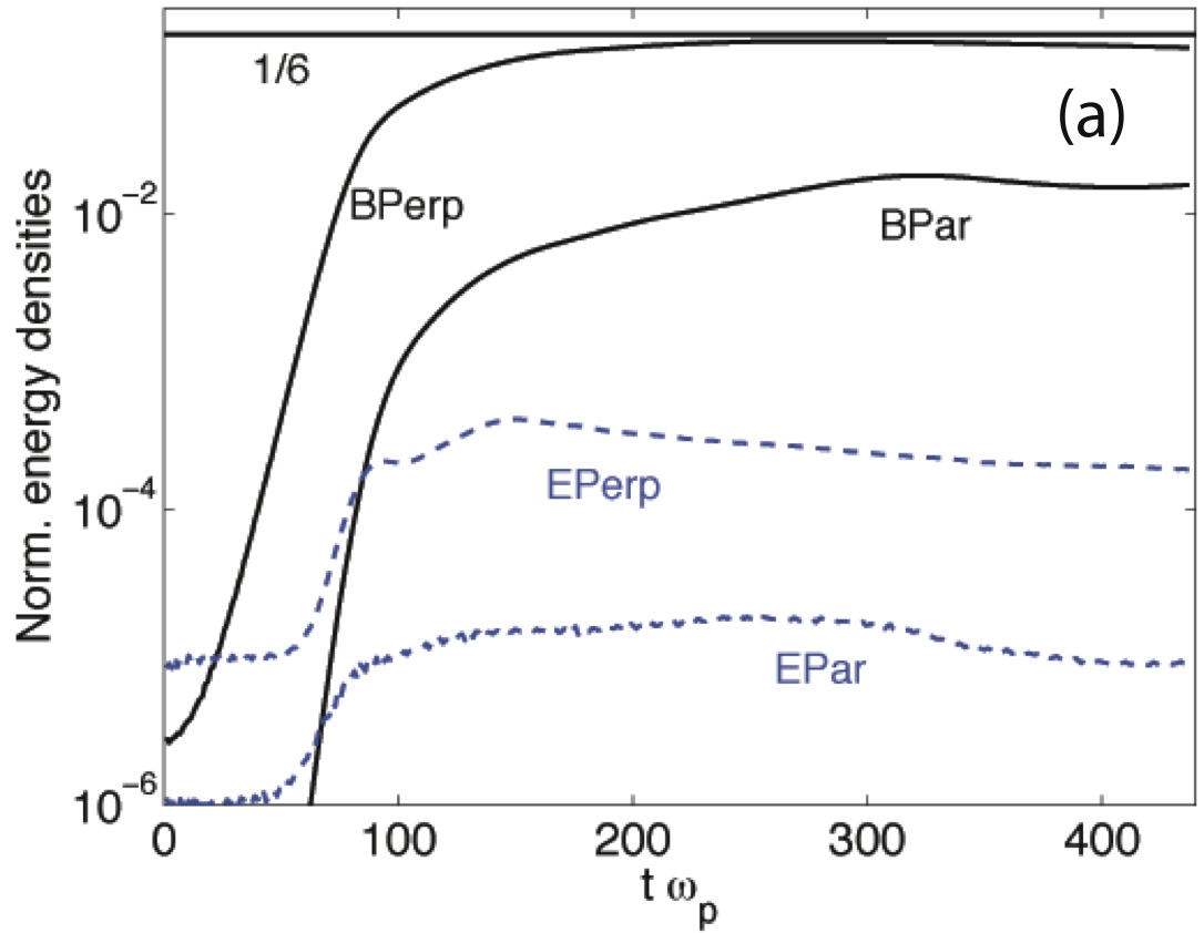
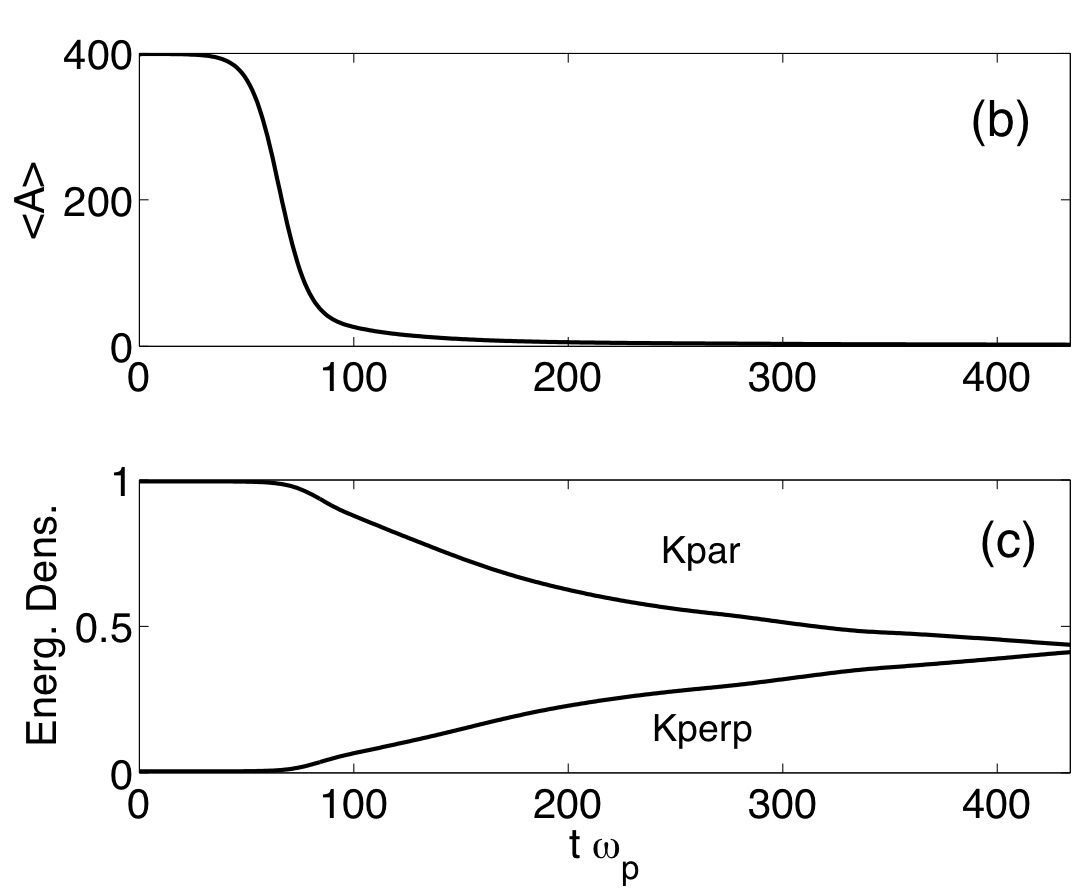
Figure 2: (Colour online) (a) The normalised magnetic energy densities $\epsilon_{B\perp}/\epsilon_{K0}$ and $\epsilon_{B\parallel}/\epsilon_{K0}$ (upper black curves) and the electric energy densities $\epsilon_{E\perp}/\epsilon_{K0}$ and $\epsilon_{E\parallel}/\epsilon_{K0}$ (lower blue dashed curves). Initially only $\epsilon_{B\perp}$ grows exponentially and the onset of its saturation at $t\omega_{p}\approx 60$ triggers the growth of the other components. The energy density of $B_{\perp}$ peaks above a value 1/12 and just below 1/6 (horizonal line). (b) The decrease of the averaged anisotropy $<A>$. (c) The kinetic energy density of particles moving in parallel and perpendicular direction.

The growth of $\epsilon_{B\perp}$ is exponential for $t\omega_{p}<60$ and we notice a weak growth of $\epsilon_{E\parallel}$, while the other energy densities are at noise levels. This defines the linear phase of the instability. The $\epsilon_{E\perp}\gg\epsilon_{E\parallel}$ at this early time, because the latter is electromagnetic in the chosen geometry, while $\epsilon_{E\perp}$ contains also electrostatic noise. After $t\omega_{p}\approx 60$ the growth of $\epsilon_{B\perp}$ slows down, while the other energy densities grow rapidly. Processes must be at work, which are not captured by the solution of the linear dispersion relation. The $\epsilon_{B\parallel}$ is amplified here, but not in a 1D simulation that evidences only a growth of $\epsilon_{E\perp}$ and of $\epsilon_{E\parallel}$[17]. All energy densities saturate at the same time at $t\omega_{p}\approx 80$. Furthermore, the energy density $\epsilon_{E\perp}$ is two to three orders of magnitude smaller than $\epsilon_{B\perp}$, thus the amplitude of the mean electric field is one to two orders of magnitude lower than the amplitude of the mean magnetic field. Most electrons have velocities well below $c/10$ and they are therefore affected by the electric force as much as by the magnetic force. Neglecting the electric field [11] is thus not necessarily permitted.

We can approximate with an exponential function the early stage of the evolution of the energy densities of the perpendicular components (not shown), yielding the growth rates $\sigma_{B\perp}\approx 0.07\omega_{p}$, which is below the analytical value $\sigma_{Ana}=0.114\omega_{p}$, while $\sigma_{E\perp}\approx 0.06\omega_{p}$. It is the same situation as in reference [17]: The growth rate of the magnetic energy density is reduced in comparison to the analytical value. This is at least partially due to the averaging over all wave numbers. The growth rate of $\epsilon_{E\perp}$ is here below that of $\epsilon_{B\perp}$, while it grew twice as fast in a 1D simulation [17]. Such a reduction of the growth rate of $\epsilon_{E\perp}$ as we go from a 1D to a 2D simulation is also observed for the FI [18].

In Figure 2 (b) the decrease of the thermal anisotropy is shown. With the transition to the nonlinear phase the thermal temperatures have almost equalized. Also the kinetic energies of particles moving in parallel and perpendicular direction balances (see Figure 2 (c)).

3.2 The power spectra of the field components

In what follows, we analyse the nonlinear evolution of the fields. Figures 3(a-c) display the power spectra of $cB_{\perp}$, $cB_{\parallel}$ and $E_{\perp}$. The power spectra as a function of the scalar wavenumber $k={(k_{x}^{2}+k_{y}^{2})}^{1/2}$ have been obtained by the integration over the azimuth angle of the power spectrum in the $k_{x}-k_{y}$ plane. We have normalised the spectra by $P_{0}$, which is the highest value of the power spectrum $P(k,t)$ of $B_{\perp}$.

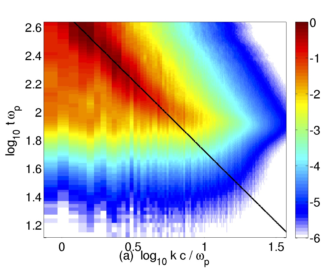
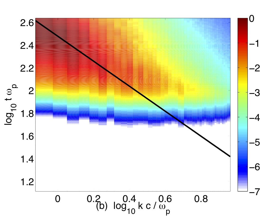
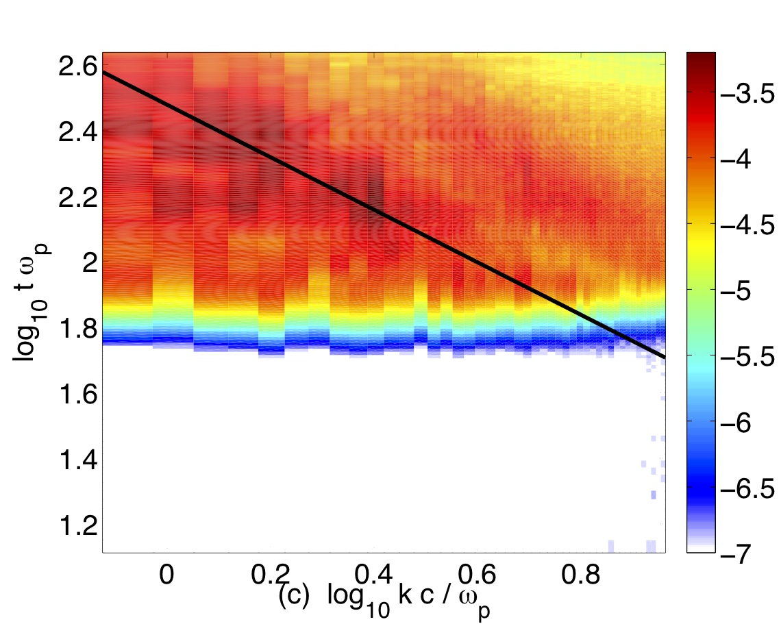
Figure 3: (Colour online) The power spectra $P(k,t)/P_{0}$ of $cB_{\perp}$ (a), $cB_{\parallel}$ (b) and $E_{\perp}$ (c) as a function of the logarithmic (base 10) wave number and time. $P_{0}$ is the maximum value of the power spectrum of $cB_{\perp}$. The colourbar is the 10-logarithm of the normalised power. The overplotted curve $k^{\prime}\propto t^{-1}$follows the evolution of the power maximum to low $k$.

The $cB_{\perp}$ grows exponentially and to a significant power over a wide range of wave numbers up to a $k=k_{max,Sim}$ with $\log_{10}(k_{max,Sim}c/\omega_{p})\approx 1.2$. This is close to the analytical value $\log_{10}(k_{max,Ana}c/\omega_{p})=\log_{10}\sqrt{A}\approx 1.3$. The $P/P_{0}$ gradually goes over into noise at higher $k$. The magnetic field components $cB_{\perp}$ and $cB_{\parallel}$ grow in a similar range of wave numbers, which suggests that they are coupled. This mechanism must be nonlinear, because the solution of the linear dispersion relation does not predict the growth of $cB_{\parallel}$. The correlation of both magnetic components is reduced at later times, when the spectrum of $cB_{\perp}$ broadens. The wavenumber spectra of $E_{\perp}$ and of $B_{\parallel}$ evidence the onset of the growth of structures at about the same time $t\omega_{p}\sim 10^{2}$. However, the power spectrum of the electric field reaches larger wave numbers. The electric field thus changes more rapidly in space than the magnetic one, as it would be the case if it were driven for example by the magnetic pressure gradient $\propto\nabla\mathbf{B}^{2}$.

Figure 3 furthermore shows that the power of the field components during the non-linear phase shifts in time to lower wave numbers $k$. This goes along with an increase of the scale size (coherence length) of the magnetic field by the merging of the current structures in position space. The merging requires two spatial dimensions orthogonal to the parallel axis [11]. In a 1D simulation the merging of the current filament eventually stalls [11, 17, 16]. The wave number associated with the maximum power of $cB_{\perp}$ can be approximated by the curve $k^{\prime}\propto t^{-1}$. However, the power spectra are broadband and the sampling time too short to determine accurately this dependence.

Figure 4: 10-logarithmic plot of the power spectrum at $t\omega_{p}=434$. The dashed lines are the fits to the simulation data.

Figure 4 is a double logarithmic plot of the power spectra of the field components $cB_{\perp}$, $cB_{\parallel}$ and $E_{\perp}$ against the normalised wave number at the end of the simulation. Only the range up to $\log_{10}(kc/\omega_{p})=1.15$ is shown here as the noise dominates at large values. The power spectra have a power-law behaviour for almost the whole range. The indices are $-5.2$ for $cB_{\perp}$, $-5.4$ for $cB_{\parallel}$ and $-0.9$ for $E_{\perp}$. The power spectra of $B_{\perp}$ and $B_{\parallel}$ are practically identical, except for a scaling factor $\approx 10$. This is further evidence for a nonlinear coupling between both components. In contrast, the power spectrum of the electric field is flat compared to the magnetic components. The amplitudes for $cB_{\perp},cB_{\parallel}$ and $E_{\perp}$ are proportional to a force. The spectral distributions reveal a trend, namely that the electric forces can become more important than the magnetic ones, if the dynamics of non-relativistic electrons on small scales (large $k$) is considered.

3.3 The saturation mechanism

The field data are now analyzed in order to give information about the saturation mechanism and about how the driving field $B_{\perp}$ couples to $E_{\perp}$ and to $B_{\parallel}$. We consider for this purpose the equation

$$\partial_{t}(n\mathbf{v})+\nabla\cdot(n\mathbf{v}\mathbf{v})=-\frac{1}{m_{e}}\nabla\cdot\hat{P}_{T}-\frac{en}{m}(\mathbf{E}+\mathbf{v}\times\mathbf{B}),$$ (5)

with which we can investigate the interplay of the field components. It describes the spatio-temporal evolution of a single-species fluid consisting of electrons with particle density $n$, mean velocity $\mathbf{v}$ and thermal pressure tensor $\hat{P}_{T}$. With Ampere’s law $\mathbf{J}=\frac{1}{\mu_{0}}\nabla\times\mathbf{B}-\epsilon_{0}\frac{\partial\mathbf{E}}{\partial t}$, $\mathbf{J}=-en\mathbf{v}$ and $(\nabla\times\mathbf{B})\times\mathbf{B}=-\left[\nabla\mathbf{B}^{2}/2-\nabla\cdot(\mathbf{B}\mathbf{B})\right]$ the equation can be rewritten as

$$\partial_{t}(n\mathbf{v})+\nabla\cdot(n\mathbf{v}\mathbf{v})=-\frac{1}{m_{e}}\nabla\cdot\hat{P}_{T}-\frac{en}{m}\mathbf{E}-\frac{1}{m}\nabla\cdot\hat{\sigma}-\frac{1}{m}\nabla P_{B}+\frac{\epsilon_{0}}{m}\mathbf{B}\times\frac{\partial\mathbf{E}}{\partial t}$$ (6)

where $\hat{\sigma}=\mathbf{B}\mathbf{B}/\mu_{0}$ and $P_{B}=\mathbf{B}^{2}/2\mu_{0}$ describe the magnetic stress tensor and pressure.

If we consider a configuration where the gradients $\partial_{y}$ and $\partial_{z}$ are not resolved, the term $-\nabla\cdot\hat{\sigma}/m$ due to the magnetic tension vanishes. The development of the FI or the TAWI imply, that the term $m^{-1}\nabla P_{B}$ on the right hand side of Eq. 6 becomes important. The PIC simulations in [17, 18] demonstrate that an electric field grows with an amplitude that cancels the term $m^{-1}\nabla P_{B}$ by the second term $en\mathbf{E}/m$ on the right hand side of Eq. 6, provided that immobile ions are considered. The amplitude of the electric field along the 1D simulation box is then given by

$$E_{x}=-\frac{1}{2en_{e}\mu_{0}}\,\frac{d}{dx}B^{2}=-\frac{1}{en_{e}}\frac{d}{dx}P_{B}$$ (7)

As a result, the electric field energy density grows twice as fast as the magnetic one. The TAWI and FI saturate, when the combined electric and magnetic force prevents a further spatial re-arrangement of the current by confining the electrons in space.

The perpendicular gradients are resolved ($\partial_{x}\not=0$, $\partial_{y}\not=0$) in our 2D PIC simulation and $\nabla\cdot\hat{\sigma}$ no longer vanishes. If we neglect the contribution of the thermal pressure gradient and the displacement current (term 1 and 5 on the right hand side in Eq. 6), then the right hand side of Eq. 6 vanishes, provided that

$$\mathbf{E}_{\perp}=\frac{1}{en}\nabla_{xy}\cdot\hat{\sigma}-\frac{1}{en}\nabla_{xy}P_{B},$$ (8)

where $\nabla_{xy}$ is the gradient in the x-y plane. We will examine here the magnitude of the three terms in Eq. 8 using the PIC simulation data.

Movie 1 shows the development of the individual contributions: The upper left panel shows the magnetic field $|\mathbf{B}(x,y)|$ normalised by $\omega_{p}m/e$. The middle panel shows the development of the nonlinear terms in Eq. 8 in the same normalisation $\omega_{p}m/ce$ as the electric field, i. e. the superposition of the magnetic pressure gradient $\nabla P_{B}$ and the divergence of the magnetic stress tensor $\nabla\cdot\hat{\sigma}$. The bottom panel is the normalised electric field component $E_{\perp}(x,y)$. Besides the formation of larger structures in the magnetic field $|\mathbf{B}(x,y)|$, the connection of the magnetic tension and pressure gradient force with the perpendicular electric field is obvious at various locations in Movie 1. For $t\omega_{p}>50$ structures in the electric field are contrasted with the noise background and the strongest ones correspond to the two non-linear terms we examine here.

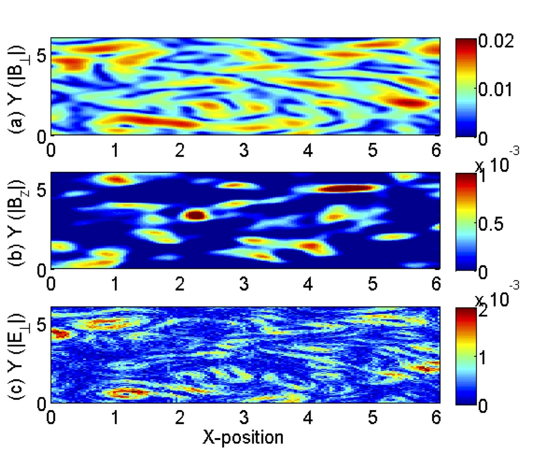
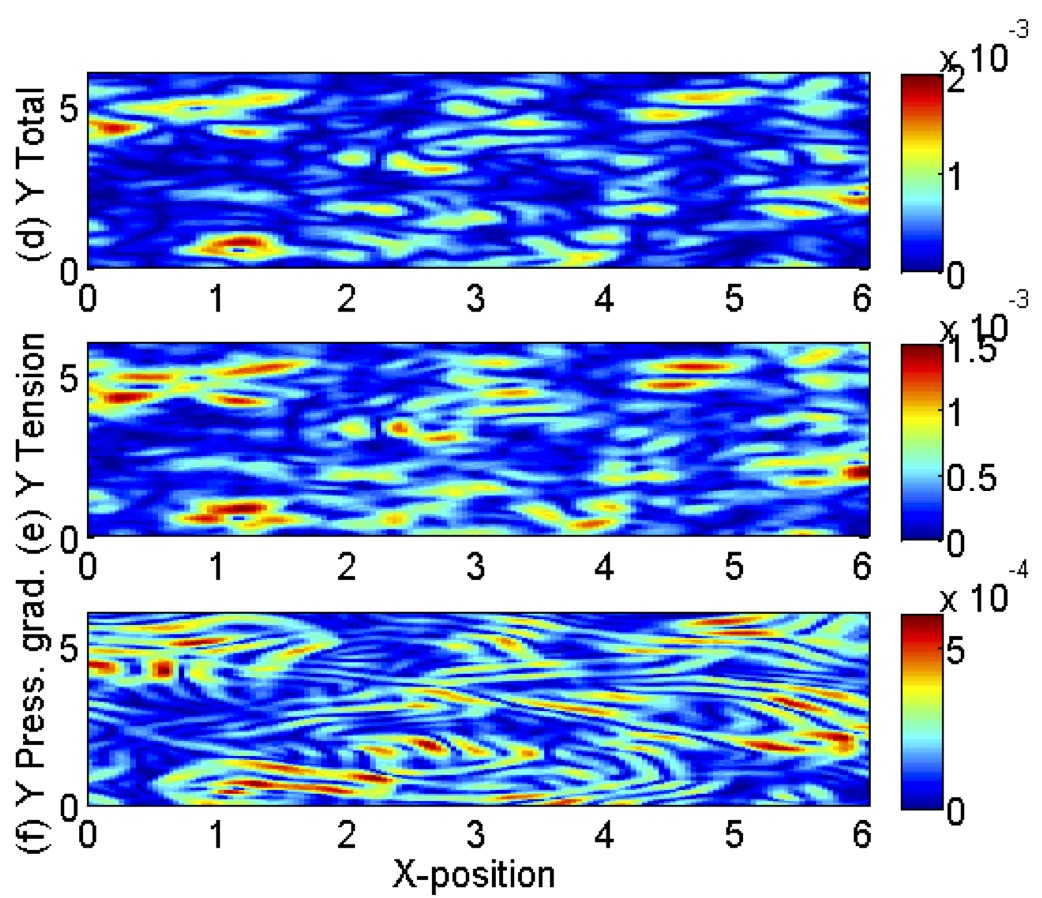
Figure 5: (Colour online) The relevant field and force components at $\omega_{p}t=75$ in a subinterval of the box: (a) $|B_{\perp}|=|B_{x}+iB_{y}|$, (b) the parallel magnetic component $|B_{\parallel}|=|B_{z}|$, (c) the $|E_{\perp}|=|E_{x}+iE_{y}|$. The force $|\nabla\cdot\hat{\sigma}+\nabla P_{B}|$ (d) and the individual components (e) $|\nabla\cdot\hat{\sigma}|$ and (f) $|\nabla P_{B}|$. Values are normalized and can be compared directly.

Figure 5 displays the most relevant field and force components at the time $\omega_{p}t=75$, when the TAWI has just saturated in Fig. 2. The dominant field component is clearly $|B_{\perp}|$, as expected from the TAWI and from the energy density diagram. The peak amplitude $\approx 0.02$ is compatible with a saturation by the magnetic trapping mechanism. The magnetic bounce frequency in the normalized units $\tilde{k}=kc/\omega_{p}$, $\tilde{v}=v/c$ and $\tilde{B}_{\perp}=mB_{\perp}/e$ displayed in Fig. 5 is $(\omega_{B}/\omega_{p})={|\tilde{k}\tilde{v}\tilde{B}_{\perp}|}^{1/2}$. We rearrange the equation and get $\tilde{v}={(\omega_{B}/\omega_{p})}^{2}/(|\tilde{B}_{\perp}|\tilde{k})$. Equating the $\omega_{B}$ with the typical growth rate from Fig. 1 gives $\omega_{B}/\omega_{p}=0.05$ and we further assume that $\tilde{k}=2.5$ and $|B_{\perp}|=0.02$. We get the reasonable rough estimate $\tilde{v}\approx 0.05$, which is a few times $v_{th\parallel}/c\approx 0.01$.

The correspondence between the total force $|\nabla\cdot\hat{\sigma}+\nabla P_{B}|$ and $|E_{\perp}|$ is apparent. The amplitudes are very similar and at least the strong structures in Figs. 5(c) and (d) agree well, e. g. at $x\omega_{p}/c=1$ and $y\omega_{p}/c=0.5$ or at $x\omega_{p}/c=0.5$ and $y\omega_{p}/c=4.5$. We find that $|E_{\perp}|\approx|B_{\perp}|/10$ in various locations and the electric force on an electron moving with the speed $c/10$ will equal the magnetic one. We decompose the total force into its constituents in Fig. 5(e,f). The major force contribution arises from the magnetic tension force. However, the omission of the magnetic pressure gradient in Fig. 5(e) alters the force distribution and results in clear differences with regard to $|E_{\perp}|$. It is thus obvious that both components provide important contributions to the total electric field. No clear connection between $B_{\parallel}$ and the other components is visible in Fig. 5.

The currents can provide further information about the coupling between $B_{\parallel}$ and the other field components. We subdivide for this purpose the current into a $J_{\parallel}=J_{z}$ and $J_{\perp}=J_{x}+iJ_{y}$. The power spectrum of both components is calculated by a 2D Fourier transform over the $x-y$ plane followed by the azimuthal integration and a normalization by the maximum power of $J_{\parallel}$. This provides us in analogy to the field distribution Fig. 3 with the time-dependent power spectra of $J_{\parallel}$ and $J_{\perp}$, which we display in Fig. 6.

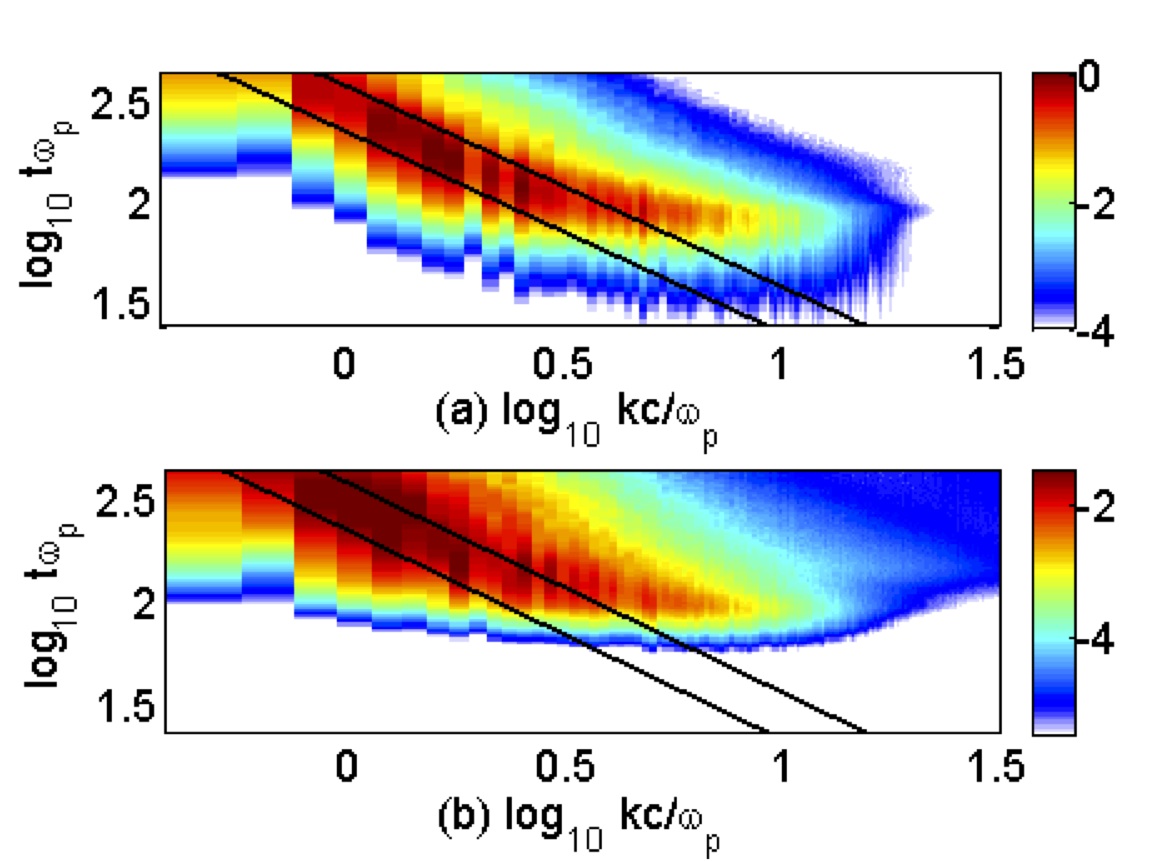
Figure 6: (Colour online) The power spectra $P(k,t)$ of the current components $J_{\parallel}$ (a) and $J_{\perp}$ (b). Both spectra are normalized to the maximum power of $J_{\parallel}$. The wavenumber, the time and the colour scale are 10-logarithmic. Overplotted are two curves $k\propto t^{-1}$, which confine the wavenumber interval with the maximum power. The curves are the same in both panels.

The expectation that $J_{\parallel}\gg J_{\perp}$ due to $|B_{\perp}|\gg|B_{\parallel}|$ is confirmed. Both current distributions reveal that the wavenumber intervals, in which the power spectra of the currents peak, can be confined by two curves that follow $k\propto t^{-1}$. The exact dependence of the wavenumbers, at which the power spectra of the currents peak is, however, not a power of $t$. The latter would correspond to a straight line in the double logarithmic diagram. Both current distributions rapidly expand to lower $k$ after $t\omega_{p}\approx 125$. This broadening of the current distribution is probably connected to that of the fields at late times in Fig. 3. A finite box effect may be responsible for this sudden broadening, because the largest observed wavelengths are not longer small compared to the box size. We discuss one such finite box effect below. However, this broadening sets in well after the saturation time $t\omega_{p}\approx 75$ and these two processes are not connected. The signal-to-noise ratio of the currents is sufficient to reveal the cut-off of both spectra at $log_{10}(kc/\omega_{p})=\log_{10}\sqrt{A}$, which is in line with Fig. 1.

The overplotted curves $k\propto t^{-1}$ show that the wavenumber intervals, in which the power spectra of both current components peak, are practically identical. This confirms their connection. The abrupt growth of the power spectrum of $J_{\perp}$ at $t\omega_{p}\approx 70$ furthermore suggests that it is caused by a non-linear process. The immobile ions imply, that the $J_{\perp}$ is caused by the bulk motion of the electrons in the simulation plane. The electrons can be accelerated either by $E_{\perp}$ or by their deflection by $B_{\perp}$ from the parallel direction into the perpendicular plane. The electromagnetic fields that accelerate the electrons in the perpendicular plane are tied to the spatially non-uniform $J_{\parallel}$, which is driven by TAWI. The fields’ extent is comparable to the spatial size of the current filaments. It is thus not surprising that the current structures in $J_{\perp}$ have a typical size that is comparable to that of the structures in $J_{\parallel}$.

The time evolution of the current distributions $J_{\parallel}(x,y)$ (upper panel) and $J_{\perp}(x,y)$ (lower panel) are shown in the movie 2 for a subsection of the simulation box. The merging of filaments in $J_{\parallel}$ can be observed. Some merge to chains. If stable chains form, that spread across the entire simulation box with its periodic boundary conditions, then this would result in finite box effects. The formation of such long chains of filaments may cause the sudden spread of the currents to low $k$ in Fig. 6 and in the electromagnetic fields in Fig. 5. The current structures in $J_{\perp}$ are driven by the fields and the current is dissipated away, resulting in their limited lifetime. The structures in $J_{\perp}$, e.g. the current eddies in the lower panel of movie 2, give rise to the $B_{\parallel}$ in Fig. 5.

3.4 The velocity distribution

The strong $J_{\parallel}$ should visibly modulate the phase space distribution $f(x,y,v_{z})$. It is, however, unclear if the phase space density remains compact or if beams form, i.e. distinct electron distributions for a given position along $x$ and $y$. Figure 7 displays the phase space distribution as a function of $v_{\parallel}(y)$ for a fixed $x\omega_{p}/c=16.8$. This phase space diagram is shown for the four simulation times $t\omega_{p}=$ 118, 198, 278 and 358. The velocity distribution, which has initially been spatially uniform, has been transformed into one, for which the mean speed varies as a function of the position. This velocity rearrangement has been accompanied by an energy transfer into the magnetic field.

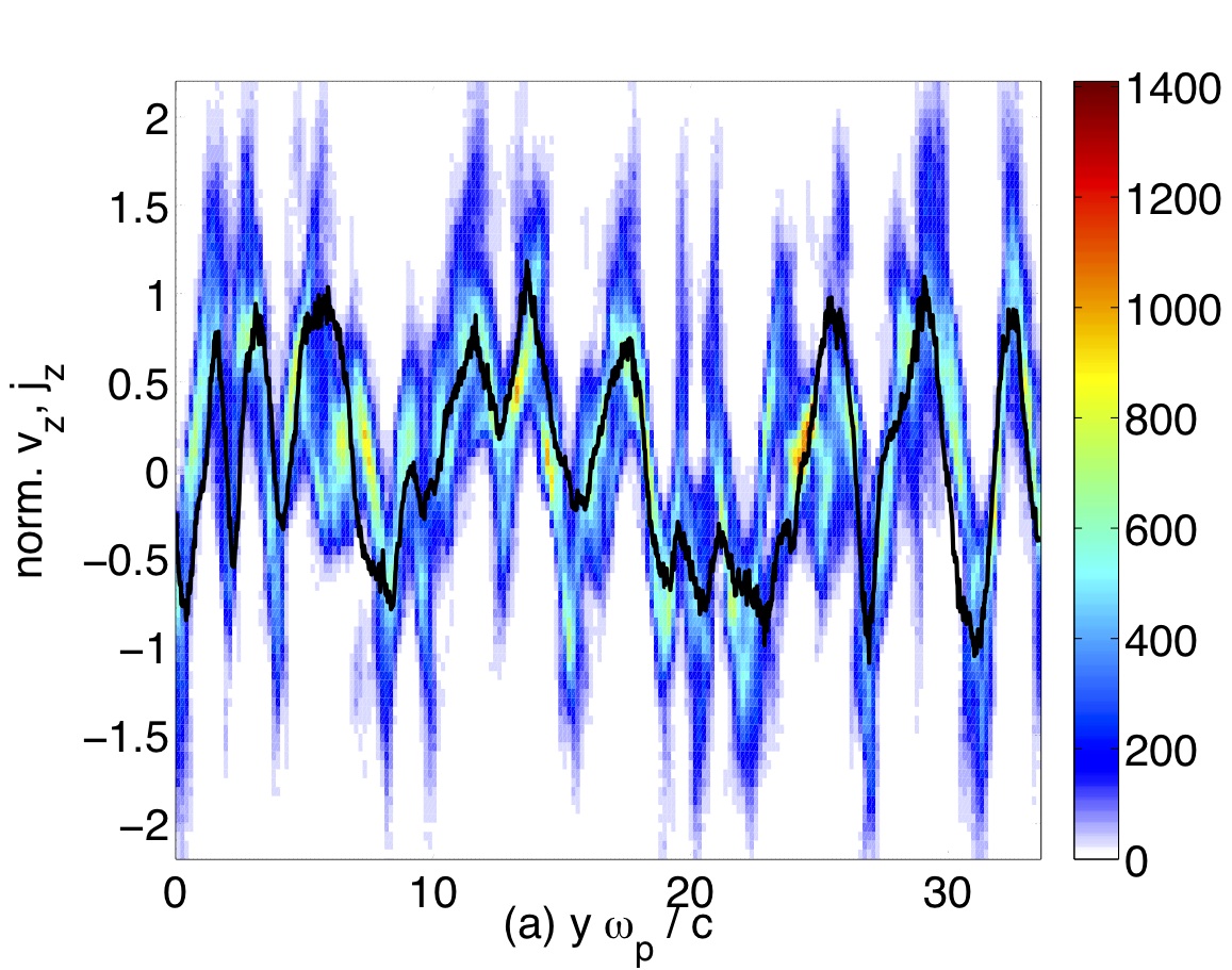
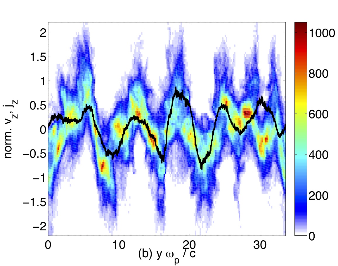
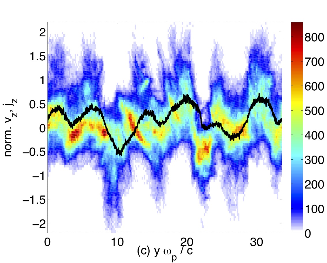
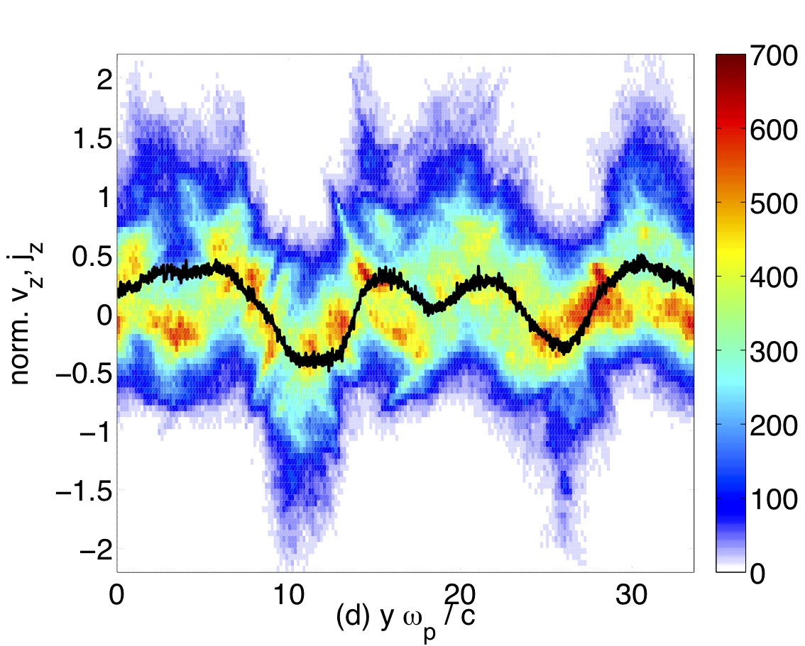
Figure 7: (Colour online) The colour plot shows the normalised velocity distribution $v_{z}(y)/v_{th\parallel}$ for $x\omega_{p}/c=16.8$ at the simulation times $t\omega_{p}=118$ (a), 198 (b), 278 (c) and 358 (d). Overplotted is the normalised current density $j_{z}(y)n_{e}/q_{cp}c$.

At $t\omega_{p}=118$, just after the TAWI has saturated, the velocity distribution oscillates in space with a high frequency, which corresponds to high $k$ in Fig. 6. The spatial oscillation frequency decreases with time, while the thermal spread of the electron beam increases. The 2D distribution is scanned along the $x$-direction shown in Movie 3 at $t\omega_{p}=358$, showing that the velocity oscillations along the slice $x\omega_{p}/c=16.8$ in Fig. 7 are representative for those in the simulation box. The actual velocity spread, within which we find significant numbers of electrons (note the linear density scale) is the same during the non-linear phase with ($|v_{z}|/v_{th\parallel}\lesssim 1.5$). Faster particles do exist. Initially the Maxwellian along the parallel direction could be populated with the given statistical plasma representation of 160 particles per cell up to $|v_{max}|\approx 2.5v_{th\parallel}$. The low number density of the fast particles implies, however, that they do not contribute much to $J_{\parallel}$. The simulation furthermore evidences, that no electrons are accelerated to high speeds during the non-linear evolution of the TAWI despite the large initial value of $A$.

The increase with time of the wave length of the spatial oscillations in Fig. 7 is related to a merging of the filaments in the $J_{\parallel}$ distribution (Movie 2), which could not be observed to this extent in the 1D simulation of our previous work [17]. In the latter work, the particles have instead been pushed together by the magnetic pressure gradient, yielding a layered structure in the velocity distributions. In our 2D simulation the filament merging destroys this effect. In agreement with these results, the structure becomes more diffuse and the normalised current density $j_{z}n_{e}/q_{cp}c=J_{z}/q_{cp}c$, overplotted in Fig. 7, with the current follows the structure of the velocity distribution.

4 Discussion

The thermal anisotropy-driven Weibel instability (TAWI), which is an important seed mechanism for magnetic fields in astrophysical environments and in laser-generated plasmas [1, 2, 10], has been investigated here with the help of a particle-in-cell (PIC) simulation for mobile electrons and for immobile ions. The plasma has initially been spatially uniform and we have set the initial electric and magnetic fields to zero. The thermal speed $v_{th\parallel}$ of the electrons along one direction has been 20 times larger than the equivalent $v_{th\perp}$ in the perpendicular plane. The anisotropy parameter $A=v_{th\parallel}^{2}/v_{th\perp}^{2}-1=399$ is thus very large. It allows us to examine the field growth and the electron thermalization under extreme conditions. It also provides us with a good signal-to-noise ratio of the electromagnetic fields in simulation. Thus, the results are valid for high anisotropies only. We plan to discuss the low anisotropy case in future work.

The main purpose of our work has been to determine the source mechanism of the electric field during the non-linear stage of the instability in more than one dimension. This electric field has recently received attention [15, 16], because the electric force is not small compared to the magnetic one. Both field components are thus important for the saturation of the TAWI, while typically only the magnetic field is considered [11, 23]. We have previously determined that the electric field is driven by the magnetic pressure gradient force, if the wave spectrum is limited to one dimension [17]. This force component is dominant for the filamentation instability in 1D and 2D simulations [18], but it was not clear if this finding holds also for the TAWI.

We summarize our results: We have compared the interval of unstable wave numbers in the simulation with the corresponding solution of the linear dispersion relation. Both agree prior to the saturation of the TAWI. Thereafter, the merging of the current filaments implies that the peak in the power spectrum of the current moves to lower wave numbers. This characteristic wave number decreases approximately linearly with an increasing time. The scale size of the filaments and the coherence length of the magnetic and the electric fields thus increases approximately linearly in time in the position space, until a sudden broadening sets in, which we have attributed to finite box effects. This evolution of the filament size contrasts the results of 1D simulations, where mergers are possible only until the magnetic field becomes strong enough to keep the filaments with oppositely directed currents separated [11, 17, 15]. The repelling filaments can go around each other in a 2D plane and they continue to merge with other filaments, which have the same direction of the current vector.

We have found that in a 2D simulation the magnetic tension force becomes stronger than the magnetic pressure gradient force, which clearly distinguishes this non-linear system from that driven by the beam filamentation instability. Both forces arise from the interaction of the net current driven by the TAWI with the magnetic field it generates. The electric field strength and distribution in the simulation plane resemble that of the force distribution obtained from the summation of the magnetic tension and pressure gradient force, at least in what concerns the strongest electric field structures. This electric field reaches an amplitude that makes it equally important for the dynamics of the slow electrons as the magnetic field. Its energy density remains, however, well below the magnetic one, which is in agreement with previous simulations. We find that the estimate for the magnetic field amplitude, which lets the TAWI saturate, that is based on the magnetic trapping mechanism is still a reasonable approximation for that observed in our simulation. This has also been reported for 1D simulations of the non-relativistic TAWI [15] and for the filamentation instability [18].

The electromagnetic fields generated by the TAWI drive electron currents in the simulation plane. These currents result in the growth of a magnetic field component, which is orthogonal to the simulation plane and parallel to the direction, along which the electrons are hottest. The growth of such a field component is not predicted by the solution of the linear dispersion relation and it is thus a purely non-linear process. This magnetic field component does also not grow in 1D PIC simulations [17]. Its amplitude is lower than that in the simulation plane but it is large enough to result in complicated 3D magnetic patterns in a 3D simulation [20].

The ratio of the energy density of the two magnetic field components in our simulation plane and the total electron thermal energy density exceeds the expected limiting value of 1/12 [12]. It remains, however, just below twice that value. Such a peak energy density of the magnetic field in the simulation plane is reasonable, if the limit 1/12 applies to each magnetic degree of freedom. One magnetic component is considered in Ref. [12], while two components grow in our simulation plane.

Acknowledgements: This work was partially supported by the Deutsche Forschungsgemeinschaft through grant Schl 201/21-1, the Research Department Plasmas with Complex Interactions at Ruhr-University Bochum and by Vetenskapsrådet. We thank the HPC2N supercomputer centre for the computer time and support.

References

References

- [1] Bell A R and Lucek S G 2001 Mon. Not. R. Astron. Soc. 321 433
- [2] Schlickeiser R and Shukla P K 2003 Astrophys. J. 599 L57
- [3] Yoon P H and Davidson R C 1987 Phys. Rev. A 35 2718
- [4] Tautz R C and Schlickeiser R 2006 Phys. Plasmas 13 062901
- [5] Achterberg A and Wiersma J 2007 Astrom. Astrophys. 475 1
- [6] Pétri J and Kirk J G 2007 Plasma Phys. Control. Fusion 49 1885
- [7] Silva L O, Fonseca R A, Tonge J W, Dawson J M, Mori W B and Medvedev M V 2003 Astrophys. J. 596 L121
- [8] Stockem A, Dieckmann M E and Schlickeiser R 2008 Plasma Phys. Control. Fusion 50 025002
- [9] Medvedev M V and Loeb A 1999 Astrophys. J. 526 697
- [10] Karmakar A, Kumar N and Pukhov A 2009 Phys. Rev. E 80 016401
- [11] Morse R L and Nielsen C W 1971 Phys. Fluids 14 830
- [12] Lemons D S, Winske D and Gary S P 1979 J. Plasma Phys. 21 287
- [13] Lemons D S and Winske D 1980 J. Plasma Phys. 23 283
- [14] Borodachev L V and Kolomiets D O 2010 J. Plasma Phys., doi:10.1017/S0022377810000188, in press
- [15] Kaang H H, Ryu C M and Yoon P H 2009 Phys. Plasmas 16 082103
- [16] Palodhi L, Califano F and Pegoraro F 2009 Plasma Phys. Controll. Fusion 51, 125006
- [17] Stockem A, Dieckmann M E and Schlickeiser R 2009 Plasma Phys. Control. Fusion 51 075014
- [18] Dieckmann M E 2009 Plasma Phys. Control. Fusion 51 124042
- [19] Dieckmann M E, Lerche I, Shukla P K and Drury L O C 2007 New J. Phys. 9 10
- [20] Romanov D V, Bychenkov V Y, Rozmus W, Capjack C E and Fedosejevs R 2004 Phys. Rev. Lett. 93 215004
- [21] Lazar M, Schlickeiser R and Shukla P K 2006 Phys. Plasmas 13 102107
- [22] Eastwood J W 1991 Comput. Phys. Comm. 64 252
- [23] Davidson R C, Hammer D A, Haber I and Wagner C E 1972 Phys. Fluids 15 317
- [24] Califano F, Cecchi T and Chiuderi C 2002 Phys. Plasmas 9 451
- [25] Rowlands G, Dieckmann M E and Shukla P K 2007 New J. Phys. 9 247