FACTORIZING THE STOCHASTIC GALERKIN SYSTEM

Abstract

Recent work has explored solver strategies for the linear system of equations arising from a spectral Galerkin approximation of the solution of PDEs with parameterized (or stochastic) inputs. We consider the related problem of a matrix equation whose matrix and right hand side depend on a set of parameters (e.g. a PDE with stochastic inputs semidiscretized in space) and examine the linear system arising from a similar Galerkin approximation of the solution. We derive a useful factorization of this system of equations, which yields bounds on the eigenvalues, clues to preconditioning, and a flexible implementation method for a wide array of problems. We complement this analysis with (i) a numerical study of preconditioners on a standard elliptic PDE test problem and (ii) a fluids application using existing CFD codes; the MATLAB codes used in the numerical studies are available online.

1 Introduction

Complex engineering models are often described by systems of equations, where the model outputs depend on a set of input parameters. Given values for the input parameters, the model output may be computed by solving a discretized differential equation, which typically involves the solution (or series of solutions) of a system of linear equations for the unknowns. Each of these computations may be very expensive depending on factors such as grid resolution or physics components in the model. As the role of simulation gains prominence in areas such as decision support, design optimization, and predictive science, understanding the effects of variability in the input parameters on variability in the model output becomes more important. Exhaustive parameter studies (e.g. uncertainty quantification, sensitivity analysis, model calibration) can be prohibitively expensive – particularly for a large number of input parameters – and therefore accurate interpolation and robust surrogate models are essential.

We consider the model problem of a matrix equation whose matrix and right hand side depend on a set of parameters. Let $s\in\mathcal{S}$ be a set of input parameters from a $d$-dimensional tensor product parameter space $\mathcal{S}=\mathcal{S}_{1}\otimes\cdots\otimes\mathcal{S}_{d}$; the range of each $\mathcal{S}_{i}$ may be bounded or unbounded. We equip the parameter space with a bounded, separable, positive weight function $\omega:\mathcal{S}\mapsto\mathbb{R}_{+}$, where $\omega(s)=\omega_{1}(s_{1})\cdots\omega_{d}(s_{d})$. (In a probabilistic context, this weight function represents a probability measure on the input parameter space.) Let $A(s)$ be an $N\times N$ matrix-valued function where we assume that $A(s)$ is invertible for all $s\in\mathcal{S}$, and let $b(s)$ be the vector-valued function with $N$ components, where each component is square integrable with respect to $\omega$. We seek the vector valued function $x(s)$ that satisfies

$$A(s)x(s)=b(s),\qquad s\in\mathcal{S}.$$ (1)

Such parameterized matrix problems often arise as an intermediate step when computing an approximate solution of a complex model with multiple input parameters. They appear in such diverse fields as differential equations with random (or parameterized) inputs [1, 34], electronic circuit design [26], image deblurring models [5], and ranking methods for nodes in a graph [28, 8]. Given a parameterized matrix equation, one may wish to approximate the vector valued function that satisfies the equation or estimate its statistics. Once an approximation is constructed that is cheaper to evaluate than the true solution, statistics – such as mean and variance – of the approximation represent estimates of statistics of the true solution.

The approximation model is a vector of multivariate polynomials represented as a series of orthonormal polynomial basis functions where each basis function is a product of univariate orthonormal polynomials. We employ the standard multi-index notation; let $\alpha=(\alpha_{1},\dots,\alpha_{d})\in\mathbb{N}^{d}$ be a multi-index, and define the basis polynomial

$$\pi_{\alpha}(s)=\pi_{\alpha_{1}}(s_{1})\cdots\pi_{\alpha_{d}}(s_{d}).$$ (2)

The polynomial $\pi_{\alpha_{i}}(s_{i})$ is the orthonormal polynomial of degree $\alpha_{i}$, where the orthogonality is defined with respect to the weight function $\omega_{i}(s_{i})$. Then for $\alpha,\beta\in\mathbb{N}^{d}$,

$$\int_{\mathcal{S}}\pi_{\alpha}(s)\pi_{\beta}(s)\omega(s)\,ds=\left\{\begin{array}[]{cl}1,&\alpha=\beta\\ 0,&\mbox{otherwise}\end{array}\right.$$ (3)

where equality between multi-indicies means component-wise equality. For a given index set $\mathcal{I}\subset\mathbb{N}^{d}$ with size $|\mathcal{I}|<\infty$, the polynomial approximation can be written

$$x(s)\;\approx\;\sum_{\alpha\in\mathcal{I}}\mathbf{x}_{\alpha}\pi_{\alpha}(s)\;=\;\mathbf{X}\mbox{\boldmath$\pi$}(s).$$ (4)

The $N$-vector $\mathbf{x}_{\alpha}$ is the coefficient of the series corresponding to $\pi_{\alpha}(s)$. The $N\times|\mathcal{I}|$ matrix $\mathbf{X}$ has columns $\mathbf{x}_{\alpha}$, and the parameterized vector $\mbox{\boldmath$\pi$}(s)$ contains the basis polynomials. The goal of the approximation method is to compute the unknown coefficients $\mathbf{X}$.

Such polynomial models have become popular for approximating the solution of PDEs with random inputs [24, 39]; they appear under names such as polynomial chaos methods [41], stochastic finite element methods [19], stochastic Galerkin methods [3], and stochastic collocation methods [40, 2]. The Galerkin methods compute the series coefficients such that the equation residual is orthogonal to the approximation space defined by the index set $\mathcal{I}$; they typically employ a full polynomial basis of order $n$ given by

$$\mathcal{I}\;=\;\mathcal{I}_{n}\;=\;\{\alpha\in\mathbb{N}^{d}\;:\;\alpha_{1}+\cdots+\alpha_{d}\leq n\},$$ (5)

although such a basis set is not strictly necessary. The number of terms in this basis set is $|\mathcal{I}_{n}|=\binom{n+d}{n}$, which grows rapidly for $d>1$. The process of computing the coefficients involves solving a linear system of size $N|\mathcal{I}|\times N|\mathcal{I}|$, which can be prohibitively large for even a moderate number of input parameters (6 to 10) and low order polynomials (degree $<5$). For this reason, there has been a flurry of recent work on solver strategies for the matrix equations arising from the Galerkin methods [30, 35, 23, 12, 11, 14, 36], including papers on preconditioning [33, 13, 32, 37]. Such work has relied on knowing the matrix valued coefficients $\mathbf{A}_{\alpha}$ of a series expansion of the parameterized matrix $A(s)$,

$$A(s)=\sum_{\alpha}\mathbf{A}_{\alpha}\pi_{\alpha}(s),$$ (6)

which typically come from a specific form of the coefficients of the elliptic operator in the PDE models. Another drawback of the Galerkin method is its limited ability to take advantage of existing solvers for the problem $A(\lambda)x(\lambda)=b(\lambda)$ given a parameter point $\lambda\in\mathcal{S}$. In contrast, the pseudospectral and collocation methods can compute coefficients of the model (4) using only evaluations of the solution vector $x(\lambda)$. The chosen points typically correspond to a multivariate quadrature rule, and computing the coefficients of the polynomial model (4) becomes equivalent to approximating its Fourier coefficients with the quadrature rule [2, 9]. Thus, from the point of view of code reuse and rapid implementation, the pseudospectral/collocation methods have a distinct advantage.

We propose a variant of the Galerkin method that alleviates the drawbacks of limited code reuse and memory limitations. By formally replacing the integration in the Galerkin method by a multivariate quadrature rule – a step that is more often than not performed in practice – we derive a decomposition of the linear system of equations used to compute the Galerkin coefficients of (4); such a method has been called Galerkin with numerical integration in the context of numerical methods for PDEs [4]. This decomposition allows us to compute the Galerkin coefficients using only evaluations of the parameterized matrix $A(\lambda)$ and parameterized vector $b(\lambda)$ for points $\lambda\in\mathcal{S}$ corresponding to a quadrature rule. In fact, if one requires only matrix-vector multiplies as in Krylov-based iterative methods (e.g. cg [22] or minres [29] solvers) for the Galerkin system of equations, this restriction can be relaxed to matrix-vector products $A(\lambda)\mathbf{v}$ for a given $N$-vector $\mathbf{v}$; there is no need for the coefficients of an expansion of $A(s)$ as in (6). Therefore the method takes full advantage of sparsity of the parameterized system resulting in reduced memory requirements. The decomposition also yields insights for preconditioning the Galerkin system that generalize existing work. Additionally, the decomposition immediately reveals bounds on the eigenvalues of the Galerkin system for the case of symmetric $A(s)$.

The remainder of the paper is structured as follows. In Section 2, we derive the Galerkin method for a given problem and basis set. We then derive the decomposition of the matrix used to compute the Galerkin coefficients and examine its consequences including bounds on the eigenvalues of the matrix, strategies for simple implementation and code reuse, and insights into preconditioning. We then provide a numerical study of various preconditioners suggested by the decomposition using the common test case of an elliptic PDE with parameterized coefficients in Section 3; the codes for the numerical study are available in a Matlab suite of tools accessible online [20]. To emphasize the advantages of code reuse, we apply the method to an engineering test problem using existing codes in Section 4. Finally, we conclude in Section 5 with summarizing remarks.

1.1 Notation

For the remainder of the paper, we will use the bracket notation $\left\langle\cdot\right\rangle$ to denote a discrete approximation to the integral with respect to the weight function $\omega$. In other words, for functions $f:\mathcal{S}\longrightarrow\mathbb{R}$,

$$\int_{\mathcal{S}}f(s)\omega(s)\,ds\;\approx\;\sum_{\beta\in\mathcal{J}}f(\lambda_{\beta})\nu_{\beta}\;\equiv\;\left\langle f\right\rangle,$$ (7)

where the points $\lambda_{\beta}=(\lambda_{\beta_{1}},\dots,\lambda_{\beta_{d}})\in\mathcal{S}$ and weights $\nu_{\beta}\in\mathbb{R}_{+}$ define a multivariate quadrature rule for multi-indicies in the set $\mathcal{J}\subset\mathbb{N}^{d}$. We will abuse this notation by putting matrix and vector valued functions inside the brackets, as well. For example, $\left\langle A\right\rangle$ denotes the mean of $A(s)$ computed with a quadrature rule.

2 A Spectral Galerkin Method

We first review the Galerkin method [9] for computing the coefficients of the polynomial model (4). Define the residual

$$r(y,s)=A(s)y(s)-b(s),$$ (8)

and let $x_{g}(s)$ be the Galerkin approximation. Denote the $i$th component of the residual by $r_{i}(x_{g},s)$. We require that each component of the residual be orthogonal to the approximation space defined by the span of $\pi_{\alpha}$ with $\alpha\in\mathcal{I}$,

$$\left\langle r_{i}(x_{g})\pi_{\alpha}\right\rangle=0,\qquad i=1,\dots,N,\qquad\alpha\in\mathcal{I}.$$ (9)

We can combine the equations in (9) using the matrix notation

$$\left\langle r(x_{g})\mbox{\boldmath$\pi$}^{T}\right\rangle\;=\;\left\langle(Ax_{g}-b)\mbox{\boldmath$\pi$}^{T}\right\rangle\;=\;\mathbf{0},$$ (10)

or equivalently, upon substituting the model $x_{g}(s)=\mathbf{X}\mbox{\boldmath$\pi$}(s)$,

$$\left\langle A\mathbf{X}\mbox{\boldmath$\pi$}\mbox{\boldmath$\pi$}^{T}\right\rangle=\left\langle b\mbox{\boldmath$\pi$}^{T}\right\rangle.$$ (11)

Using the vec notation [21, Section 4.5], we can rewrite (11) as

$$\left\langle\mbox{\boldmath$\pi$}\mbox{\boldmath$\pi$}^{T}\otimes A\right\rangle\mathbf{x}=\left\langle\mbox{\boldmath$\pi$}\otimes b\right\rangle.$$ (12)

where $\mathbf{x}=\mathrm{vec}(\mathbf{X})$ is an $N|\mathcal{I}|\times 1$ constant vector equal to the columns of $\mathbf{X}$ stacked on top of each other. The constant matrix $\left\langle\mbox{\boldmath$\pi$}\mbox{\boldmath$\pi$}^{T}\otimes A\right\rangle$ has size $N|\mathcal{I}|\times N|\mathcal{I}|$ and a distinct block structure; the $\alpha,\beta$ block of size $N\times N$ is equal to $\left\langle\pi_{\alpha}\pi_{\beta}A\right\rangle$ for multi-indicies $\alpha,\beta\in\mathcal{I}$. Similarly, the $\alpha$ block of the $N|\mathcal{I}|\times 1$ vector $\left\langle\mbox{\boldmath$\pi$}\otimes b\right\rangle$ is equal to $\left\langle b\pi_{\alpha}\right\rangle$, i.e. the Fourier coefficient of $b$ associated with $\pi_{\alpha}(s)$ approximated with the quadrature rule.

Much of the literature on PDEs with random inputs [30, 33] points out an interesting block sparsity pattern that arises in the matrix $\left\langle\mbox{\boldmath$\pi$}\mbox{\boldmath$\pi$}^{T}\otimes A\right\rangle$ when the parameterized matrix $A(s)$ depends at most linearly on any components of $s$ and integrals are computed exactly; this is a result the orthogonality of the bases $\mbox{\boldmath$\pi$}(s)$. For general analytic dependence on the parameters, such sparsity patterns do not appear [15]. However, one can always mimick the sparsity pattern of $A(s)$ with a simple reordering of the variables. By taking the transpose of (11) and using the same vec operations, if we define $\tilde{\mathbf{x}}=\mathrm{vec}(\mathbf{X}^{T})$ (i.e. the same unknowns reordered), then

$$\left\langle A\otimes\mbox{\boldmath$\pi$}\mbox{\boldmath$\pi$}^{T}\right\rangle\tilde{\mathbf{x}}=\left\langle b\otimes\mbox{\boldmath$\pi$}\right\rangle.$$ (13)

Notice that the matrix in (13) retains the sparsity of $A(s)$ in its blocks, since each $i,j$ block of size $|\mathcal{I}|\times|\mathcal{I}|$ is equal to $\left\langle A_{ij}\mbox{\boldmath$\pi$}\mbox{\boldmath$\pi$}^{T}\right\rangle$, where $A_{ij}(s)$ is the $i,j$ element of $A(s)$. For the remainder of the paper, however, we will work with the form (12).

By writing out the numerical integration rule for the integrals used to form $\left\langle\mbox{\boldmath$\pi$}\mbox{\boldmath$\pi$}^{T}\otimes A\right\rangle$, we uncover an interesting decomposition, which we state as a theorem.

Theorem 1.

Let $\{(\lambda_{\beta},\nu_{\beta})\}$ with $\beta\in\mathcal{J}$ be a multivariate quadrature rule. The matrix $\left\langle\mbox{\boldmath$\pi$}\mbox{\boldmath$\pi$}^{T}\otimes A\right\rangle$ can be decomposed as

$$\left\langle\mbox{\boldmath$\pi$}\mbox{\boldmath$\pi$}^{T}\otimes A\right\rangle=(\mathbf{Q}\otimes\mathbf{I})A(\mbox{\boldmath$\lambda$})(\mathbf{Q}\otimes\mathbf{I})^{T},$$ (14)

where $\mathbf{I}$ is the $N\times N$ identity matrix, and $\mathbf{Q}$ is a matrix of size $|\mathcal{I}|\times|\mathcal{J}|$ – one row for each basis polynomial and one column for each point in the quadrature rule. The matrix $A(\mbox{\boldmath$\lambda$})$ is a block diagonal matrix of size $N|\mathcal{J}|\times N|\mathcal{J}|$ where each nonzero block is $A(\lambda_{\beta})$ for $\beta\in\mathcal{J}$.

Proof.

Writing out the quadrature rules,

$$\left\langle\mbox{\boldmath$\pi$}\mbox{\boldmath$\pi$}^{T}\otimes A\right\rangle=\sum_{\beta\in\mathcal{J}}\left[\mbox{\boldmath$\pi$}(\lambda_{\beta})\mbox{\boldmath$\pi$}(\lambda_{\beta})^{T}\otimes A(\lambda_{\beta})\right]\nu_{\beta}.$$ (15)

Notice that the elements of the vector $\mbox{\boldmath$\pi$}(\lambda_{\beta})$ are the polynomials $\pi_{\alpha}(s)$ evaluated at the quadrature point $\lambda_{\beta}$. If we define the vectors

$$\mathbf{q}_{\beta}=\sqrt{\nu_{\beta}}\mbox{\boldmath$\pi$}(\lambda_{\beta}),$$ (16)

then we have

$$\left\langle\mbox{\boldmath$\pi$}\mbox{\boldmath$\pi$}^{T}\otimes A\right\rangle=\sum_{\beta\in\mathcal{J}}\mathbf{q}_{\beta}\mathbf{q}_{\beta}^{T}\otimes A(\lambda_{\beta}).$$ (17)

Let $\mathbf{Q}$ be the matrix whose columns are $\mathbf{q}_{\beta}$, and define the block diagonal matrix $A(\mbox{\boldmath$\lambda$})$ with diagonal blocks equal to $A(\lambda_{\beta})$. Then for an $N\times N$ identity matrix $\mathbf{I}$, we can rewrite (17) as (14), as required. ∎

As an aside, we note that if $A(s)$ depends polynomially on the parameters $s$, then each integrand in the matrix $\left\langle\mbox{\boldmath$\pi$}\mbox{\boldmath$\pi$}^{T}\otimes A\right\rangle$ is a polynomial in $s$. Therefore by the polynomial exactness, there is a Gaussian quadrature rule such that the numerical integration approach exactly recovers the true Galerkin matrix.

The elements of $\mathbf{Q}$ are the orthogonal polynomials evaluated at the quadrature points and multiplied by the square root of the quadrature weights. They are intimately related to the normalized eigenvectors of the symmetric, tridiagonal Jacobi matrices of the three-term recurrence coefficients of the orthogonal polynomials, which can be computed efficiently by methods for computing eigenvectors; see [18, 9] and Appendix A for more details. For two polynomials $\pi_{\alpha}(s)$ and $\pi_{\beta}(s)$ with $\alpha,\beta\in\mathcal{I}$, define $\mathbf{r}_{\alpha}$ and $\mathbf{r}_{\beta}$ to be the corresponding rows of $\mathbf{Q}$; then

$$\mathbf{r}_{\alpha}\mathbf{r}_{\beta}^{T}=\sum_{\gamma\in\mathcal{J}}\pi_{\alpha}(\lambda_{\gamma})\pi_{\beta}(\lambda_{\gamma})\nu_{\gamma}.$$ (18)

If the quadrature rule is a tensor product Gaussian quadrature rule of sufficiently high order to exactly compute the polynomial integrand, then this implies $\mathbf{Q}\mathbf{Q}^{T}=\mathbf{I}$, where $\mathbf{I}$ is the $|\mathcal{I}|\times|\mathcal{I}|$ identity matrix; we will assume from here on that the chosen quadrature rule yields this property. We will also assume that the number of basis polynomials is less than the number of points used in the quadrature rule, i.e. $|\mathcal{I}|\leq|\mathcal{J}|$; otherwise the Galerkin matrix $\left\langle\mbox{\boldmath$\pi$}\mbox{\boldmath$\pi$}^{T}\otimes A\right\rangle$ will be rank deficient.

Theorem 1 reveals bounds on the eigenvalues of the matrix $\left\langle\mbox{\boldmath$\pi$}\mbox{\boldmath$\pi$}^{T}\otimes A\right\rangle$ for the case when $A(s)$ is symmetric; we state this as a corollary.

Corollary 2.

Suppose $A(s)$ is symmetric for all $s\in\mathcal{S}^{d}$. The eigenvalues of $\left\langle\mbox{\boldmath$\pi$}\mbox{\boldmath$\pi$}^{T}\otimes A\right\rangle$ satisfy the bounds

$$\min_{\beta\in\mathcal{J}}\left[\theta_{\mathrm{min}}\Bigl{(}A(\lambda_{\beta})\Bigr{)}\right]\;\leq\;\theta\Bigl{(}\left\langle\mbox{\boldmath$\pi$}\mbox{\boldmath$\pi$}^{T}\otimes A\right\rangle\Bigr{)}\;\leq\;\max_{\beta\in\mathcal{J}}\left[\theta_{\mathrm{max}}\Bigl{(}A(\lambda_{\beta})\Bigr{)}\right],$$ (19)

where $\theta(X)$ denotes the eigenvalues of a matrix $X$, and $\theta_{\mathrm{min}}(X)$ and $\theta_{\mathrm{max}}(X)$ denote the smallest and largest eigenvalues of $X$, respectively.

The proof of Corollary 2 involves a detailed discussion of the properties of orthogonal polynomials and the tridiagonal matrices of their three-term recurrence coefficients. To keep this section focused, we have placed the proof in an appendix along with a note on the sharpness of the bounds. To conclude this section, we note that if $A(s)$ is positive definite for all $s\in\mathcal{S}$, then Corollary 2.2 implies that $\left\langle\mbox{\boldmath$\pi$}\mbox{\boldmath$\pi$}^{T}\otimes A\right\rangle$ will be positive definite, as well.

2.1 Iterative Solvers

Due to their size and sparsity, the preferred way of solving (12) is with Krylov based iterative solvers [30] that rely on matrix-vector products with the matrix $\left\langle\mbox{\boldmath$\pi$}\mbox{\boldmath$\pi$}^{T}\otimes A\right\rangle$. By employing the decomposition in Theorem 1, we can compute these using only multiplication of the parameterized matrix evaluated at the quadrature point by a given vector. More precisely, given a vector $\mathbf{u}=\mathrm{vec}(\mathbf{U})$, suppose we wish to compute

$$\mathbf{v}\;=\;\mathrm{vec}(\mathbf{V})\;=\;(\mathbf{Q}\otimes\mathbf{I})A(\mbox{\boldmath$\lambda$})(\mathbf{Q}\otimes\mathbf{I})^{T}\mathbf{u}.$$ (20)

We accomplish this in three steps using the properties of the Kronecker product:

1. $\mathbf{W}=\mathbf{U}\mathbf{Q}$. Let $\mathbf{w}_{\beta}$ be a column of $\mathbf{W}$ with $\beta\in\mathcal{J}$.

2. For each $\beta$, $\mathbf{y}_{\beta}=A(\lambda_{\beta})\mathbf{w}_{\beta}$. Define $\mathbf{Y}$ to be the matrix with columns $\mathbf{y}_{\beta}$.

3. $\mathbf{V}=\mathbf{Y}\mathbf{Q}^{T}$.

Step 1 can be thought of as pre-processing, and step 3 as post-processing. In practice, each row of $\mathbf{Q}$ may have a Kronecker structure corresponding to the tensor product quadrature rule. In this case, steps 1 and 3 can be computed accurately and efficiently using multiplication methods such as [16]. The second step requires only constant matrix-vector products where the matrix is $A(s)$ evaluated at the quadrature points. Therefore we can take advantage of a memory-efficient, reusable interface for the matrix-vector multiplies that will exploit any sparsity in the matrix. We reiterate that this can be accomplished without any knowledge of the specific type of parameter dependence in $A(s)$.

Each of the three steps individually admits embarrassing parallelization; steps 1 and 3 are matrix-vector multiplies with independent right hand sides, and each $\mathbf{y}_{\beta}$ in step 2 can be computed independently. However, there is substantial communication necessary between the steps, and this will be the primary barrier to parallel scalability.

The cost of this method depends on the number of basis polynomials in the approximation and number of points in the quadrature rule. Steps 1 and 3 each require $N|\mathcal{I}||\mathcal{J}|$ multiplies. If a matrix-vector product with $A(s)$ takes $\mathcal{O}(N)$ operations due to its sparsity pattern, then step 2 takes $\mathcal{O}(|\mathcal{J}|N)$ operations. Methods based on the series expansion (6) of $A(s)$ can be significantly cheaper – depending on the number of terms in (6), and assuming the so-called triple products are precomputed before the iterative solver is applied. The trade-off between cost and flexibility must be assessed per application.

2.2 Preconditioning Strategies

The number of iterations required to achieve a given convergence criterion (e.g. a sufficiently small residual) can be greatly reduced for Krylov-based iterative methods with a proper preconditioner. In general, preconditioning a system is highly problem dependent and begs for the artful intuition of the scientist. However, the structure revealed by the decomposition from Theorem 1 offers a number of useful clues.

Suppose we have an $N\times N$ matrix $\mathbf{P}$ that is easily invertible. We can construct a block-diagonal preconditioner $\mathbf{I}\otimes\mathbf{P}^{-1}$, where $\mathbf{I}$ is the identity matrix of size $|\mathcal{I}|\times|\mathcal{I}|$. If we premultiply the preconditioner against the factored form of $\left\langle\mbox{\boldmath$\pi$}\mbox{\boldmath$\pi$}^{T}\otimes A\right\rangle$, we get

$$(\mathbf{I}\otimes\mathbf{P}^{-1})(\mathbf{Q}\otimes\mathbf{I})A(\mbox{\boldmath$\lambda$})(\mathbf{Q}\otimes\mathbf{I})^{T}=(\mathbf{Q}\otimes\mathbf{I})(\mathbf{I}\otimes\mathbf{P}^{-1})A(\mbox{\boldmath$\lambda$})(\mathbf{Q}\otimes\mathbf{I})^{T}.$$ (21)

By the mixed product property and commutativity of the identity matrix, the block-diagonal preconditioner slips past $\mathbf{Q}\otimes\mathbf{I}$ to act directly on the parameterized matrix evaluated at the quadrature points. The blocks on the diagonal of the inner matrix product are $\mathbf{P}^{-1}A(\lambda_{\beta})$ for $\beta\in\mathcal{J}$. In other words, we can choose one constant matrix $\mathbf{P}$ to affect the parameterized system at all quadrature points.

A reasonable and popular choice is the mean $\mathbf{P}=\left\langle A\right\rangle$; see [32, 30] for a detailed analysis of this preconditioner for stochastic finite element systems. Notice that this is also the first $N\times N$ block of the Galerkin matrix. However, if $A(s)$ is very large or has some complicated parametric dependence, then forming the mean system and inverting it (or computing partial factors) for the preconditioner may be prohibitively expensive. If the dependence of $A(s)$ on $s$ is close to linear, then $\mathbf{P}=A\left(\left\langle s\right\rangle\right)$ may be much easier to evaluate and just as effective.

One goal of the preconditioner is reduce the condition number of the matrix, and one way of achieving this is to reduce the spread of the eigenvalues. If we knew a priori which region of the parameter space produced the extrema of the parameterized eigenvalues of $A(s)$ (e.g. the boundaries), then we could choose an appropriate parameter value to construct an effective preconditioner. Unfortunately, we only get to use one such evaluation. Therefore, if the largest possible value of the parameterized eigenvalues is very large, we may choose this parameter value. Alternatively, if the smallest eigenvalue over the parameter space is close to zero (for positive definite systems), then this may be better reduce the condition number of the Galerkin system than the parameter that produces largest eigenvalue. In the next section, we explore a few choices for the preconditioner $\mathbf{P}$ on a standard test problem.

Notice that (21) suggests two possible routes for implementing the preconditioner. If only an interface for a preconditioned matrix-vector multiply is available for the parameterized matrix, then the implementation corresponding to the right hand side of (21) is appropriate. However, this requires $|\mathcal{J}|$ applications of the preconditioner, and in all cases we expect that $|\mathcal{I}|\leq|\mathcal{J}|$. Therefore, our implementation employs the form on the left hand side of (21), which requires $|\mathcal{I}|$ applications of the preconditioner and can be computed efficiently due to its block diagonal structure.

3 Preconditioning Study

Consider the following parameterized elliptic partial differential equation with homogeneous Dirichlet boundary conditions; variations of this problem can be found in [1, 3, 17], amongst others. We seek a solution $u(x,s)$ that satisfies

$$\nabla\cdot(a(x,s)\nabla u(x,s))=1,\qquad x\in[0,1]^{2},$$ (22)

where $u=0$ on the boundary of the square domain $[0,1]^{2}$, and the parameter space is the hypercube $s\in[-1,1]^{4}$ equipped with a uniform measure. The logarithm of the elliptic coefficient is given by a truncated Karhunen-Loeve like expansion [27] of a zero-mean random field with covariance

$$C(x_{1},x_{2})=2\exp(-\|x_{1}-x_{2}\|^{2}/2),$$ (23)

so that

$$\log(a(x,s))=2\sum_{k=1}^{4}\sigma_{k}\psi_{k}(x)s_{k},$$ (24)

where $\{\sigma_{k}^{2},\psi_{k}\}$ are the eigenpairs of the covariance function. We discretize (22) using the finite element method implemented in Matlab’s pde toolbox on an irregular mesh of $N=1,\!921$ triangles. We solve the eigenvalue problem with the discrete covariance matrix to compute the values of the eigenfunctions $\psi_{k}(x)$ on the given mesh. The square roots of first ten eigenvalues $\sigma_{k}$ are plotted in Figure 1; we truncate the expansion at $d=4$ to retain roughly 90% of the energy of the field. Given a point in the parameter space, the PDE Toolbox allows us to access the stiffness matrix. Therefore we can apply Matlab’s minres solver using only matrix-vector multiplies against the stiffness matrix evaluated at the quadrature points. For the polynomial basis, we use the normalized multivariate product Legendre polynomials of order 5, which includes $|\mathcal{I}|=\binom{4+5}{5}=126$ basis functions. Therefore the number of unknowns is $N|\mathcal{I}|=242,\!046$. We use a tensor product Gauss-Legendre quadrature rule of order 12 in each parameter (20,736 points) to implicitly form the Galerkin matrix; this is more than sufficient to maintain the orthogonality in the basis functions.

Fig. 1: Eigenvalues of the KL expansion. The numbers indicate the percentage of field energy captured when using that many terms in the expansion.

To test the preconditioning ideas suggested by the decomposition from Theorem 1 and equation (21), we try five different choices of $\mathbf{P}$. For each $\mathbf{P}$, we precompute the Cholesky factors to apply (21) efficiently. Figure 2 and Table 1 summarize the results, which we now explain in detail. In the first type of preconditioning, we set $\mathbf{P}=A(s_{r})$ for a random point $s_{r}$ in $[-1,1]^{4}$. To sample the likely effectiveness of any random point, we select 25 random points and evaluate each choice of $s_{r}$. Second, we set $\mathbf{P}=A(s_{\max})$ where $A(s_{\max})$ is the matrix with the largest eigenvalue in $[-1,1]^{4}$. To compute $s_{\max}$, we use up to 100 iterations of the power method to estimate the largest eigenvalue at each point in the quadrature rule, that is for each $\lambda_{\beta}$ for $\beta\in\mathcal{J}$; we also evaluate $A(s)$ for the tensor product of the endpoints as well. Third, we set $\mathbf{P}=A(s_{\min})$ where $A(s_{\min})$ is the matrix with the smallest eigenvalue in $[-1,1]^{4}$. For this computation, we use Matlab’s optimization routine fmincon and use eigs/arpack to evaluate the smallest eigenvalue [25]. Fourth, we set $\mathbf{P}=A(s_{\text{mid}})$ where $s_{\text{mid}}$ is the midpoint of the domain, which is the origin for our experiments. Fifth, and finally, we set $\mathbf{P}=\left\langle A\right\rangle$, the mean preconditioner. To evaluate the mean, we use a 2nd order quadrature rule for a fast approximation and a 5th order quadrature rule for a more exact approximation.

In Figure 2, we show the convergence of the $2$-norm of the residual for each of the preconditioning strategies, as well as no preconditioning. We only show the result from the 5th order mean based preconditioner as there was no appreciable difference in convergence. This plot clearly shows that the mean and midpoint preconditioners are excellent choices. Further note that any random point is more than two orders of magnitude better than no preconditioning at all. In fact, using a random point is better than using the point with largest eigenvalue and may compare with using the point with the smallest eigenvalue.

Next, Table 1 shows a few timing results from these experiments. We present the time taken to compute/setup the preconditioner, the average time between iterations, and the total time taken by the minres method (excluding preconditioner setup). The times are from Matlab 2010a on an Intel Core i7-960 processor (3.2 GHz, 4 cores) with 24GB of RAM. Matlab used four cores for its own multithreading and we used the Parallel Computing toolbox’s parfor construction to parallelize the matrix-vector product over 4 cores as well. By watching a processor performance meter, we observed high utilization of all four cores. However, the system’s memory was nearly exhausted by the experiment. At irregular intervals, the system would begin swapping memory to disk heavily. This behavior caused erratic timing results, especially for the two random point evaluations. On repeated runs of the experiments, we observed wall-clock time differences of up to 100 seconds for any individual result. Thus differences below this threshold are not meaningful. From these timing results, we conclude that preconditioning changes the iteration time only slightly – if at all. Furthermore, the setup times are often small when compared with the savings in runtime.

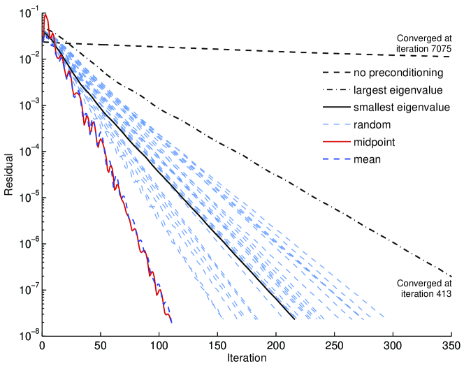
Fig. 2: Convergence of the 2-norm of the residual for a variety of preconditioners.

Table 1: Timing results for preconditioning showing only two of the random points.

Method	Setup (s)	Iterations	Avg. Iter. (s)	Total (s)
no preconditioning	0.0	7075	6.5	46251.1
largest eigenvalue	176.0	413	6.6	2810.7
smallest eigenvalue	16.0	216	6.5	1469.4
random	0.1	238	6.7	1661.8
random	0.9	216	8.4	2030.2
mean (5th order)	4.7	111	6.7	807.2
mean (2nd order)	0.7	110	6.8	820.4
midpoint	0.1	110	7.0	843.2

The Matlab codes for this study include a utility for generating realizations of random fields [10] and a suite of tools called PMPack (Parameterized Matrix Package) for using spectral methods to approximate the solution of parameterized matrix equations. The codes for generating the results of the study can be found at [20].

4 Application – Heat Transfer with Uncertain Material Properties

As a proof of concept, we examine an application from computational fluid dynamics with uncertain model inputs. The flow solver used to compute the deterministic version of this problem – i.e. for a single realization of the model inputs – was developed at Stanford’s Center for Turbulence Research as part of the Department of Energy’s Predictive Science Academic Alliance Program; the numerical method used is described in [31] and is based on an implicit, second order spatial discretization. For this example, we slightly modified the codes to extract of the non-zero elements of the matrix and right hand side used in the computation of the temperature distribution. With access to the matrix-vector multiply, we were able to apply the Galerkin method to the stochastic version of the problem to approximate the statistics of solution.

4.1 Problem Set-up

The governing equation is the integral version of a two-dimensional steady advection-diffusion equation. We seek a scalar field $\phi=\phi(x,y)$ representing the temperature defined on the domain $\Omega$ that satisfies

$$\int_{\partial\Omega}\rho\phi\left(\vec{v}(s)\cdot\vec{dS}\right)=\int_{\partial\Omega}\left(\Gamma(s)+\Gamma_{t}\right)\left(\nabla\phi\cdot\vec{dS}\right).$$ (25)

The density $\rho$ is assumed constant. The velocity $\vec{v}$ is precomputed by solving the incompressible Reynolds averaged Navier-Stokes equations and randomly perturbed by three spatially varying oscillatory functions with different frequencies such that the divergence free constraint is satisfied; the magnitudes of the perturbations are parameterized by $s_{1}$, $s_{2}$, and $s_{3}$, respectively. We interpret the magnitudes as uniform random perturbations of the velocity field, which is simply an input to this model. The diffusion coefficient $\Gamma=\Gamma(s_{4},s_{5},s_{6})$ is similarly altered by a strictly positive, parameterized, spatially varying function that models random perturbation. Collectively, the parameters $s_{1},\dots,s_{6}$ are independent and distributed uniformly over $[-1,1]$; the parameter space becomes the hypercube $[-1,1]^{6}$. The turbulent diffusion coefficient $\Gamma_{t}$ is evaluated according to the Spalart-Allmarass model [31]. The domain $\Omega$ is a channel with a series of cylinders; the computational mesh on the domain $\Omega$ contains roughly 10,000 nodes and is shown in Figure 3. Inflow and outflow boundary conditions are prescribed in the streamwise direction, and periodic boundary conditions are set along the $y$ coordinate. Specified heat flux boundary conditions are applied on the boundaries of the cylinders to model a cooling system.

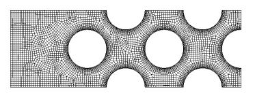
Fig. 3: Mesh used to discretize the domain $\Omega$ and compute temperature distribution.

The goal is to compute the expectation and variance of the scalar field $\phi=\phi(x,y,s)$ over the domain $\Omega$ with respect to the variability introduced by the parameters. We use the Galerkin method to construct a polynomial approximation of $\phi$ along the coordinates induced by the parameters $s$ using product Legendre polynomials. To show that this method applies for an arbitrary basis set, we choose the basis polynomials to reflect the solution’s anisotropic dependence on the parameters; it is neither the standard full polynomial or tensor product polynomial basis. The order of univariate polynomial associated with each parameter is given in Table 2, and multivariate bases are included to fall within a convex index set. The basis contains 142 multivariate polynomials; for a detailed description of the choice of bases, see [7]. To solve the Galerkin system, we use Matlab’s BiCGstab [38] method (since the matrix is not symmetric). For a preconditioner, we could only access the diagonal elements of the matrix from the solver. The results of the preconditioning study in Section 3 encouraged us to choose the midpoint of the hypercube parameter space to construct the preconditioner.

$s_{1}$	$s_{2}$	$s_{3}$	$s_{4}$	$s_{5}$	$s_{6}$
3	1	1	8	5	5

Table 2: The order of univariate polynomial for each variable used in the basis set.

We plot the expectation and variance of $\phi$ over the domain $\Omega$ in Figure 4, which are computed in the standard way as functions of the Galerkin coefficients. The variance in $\phi$ occurs in the downstream portion of the domain as a result of the variability in the diffusion coefficient.

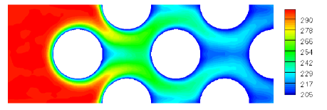
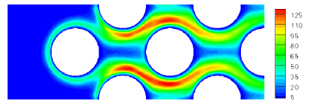
Fig. 4: The expectation (above) and variance (below) of the temperature field $\phi$ over the domain. Red corresponds to larger values and blue corresponds to smaller values.

5 Summary

We have examined the system of equations arising from a spectral Galerkin approximation of the vector valued solution $x(s)$ to the parameterized matrix equation $A(s)x(s)=b(s)$. Such problems appear when PDE models with parameterized (or random) inputs are discretized in space, and a Galerkin projection with an orthogonal polynomial basis is used for approximation in the parameter space. We showed how the system of equations used to compute the coefficients of the Galerkin approximation admits a factorization once the integration is formally replaced by a numerical quadrature rule – a common step in practice. The factorization involves (i) a matrix with orthogonal rows related to the chosen polynomial basis and numerical quadrature rule and (ii) a block diagonal matrix with nonzero blocks equal to $A(s)$ evaluated at the quadrature points. Then matrix-vector products with the Galerkin system can be computed with only the action of $A(s)$ on a vector at a point in the parameter space; this yields a reusable interface for implementing the Galerkin method. The factorization also reveals bounds on the spectrum of the Galerkin matrix, and the Kronecker structure of the factorization gives clues to successful preconditioners. We tested some ideas from these preconditioner clues on the standard test problem of an elliptic PDE with parameterized coefficients, and we saw that using $A(s)$ evaluated at the midpoint of the parameter space was as effective as the popular mean-based preconditioner; the midpoint preconditioner is much easier to compute, in general. As a proof of concept, we applied the method to an engineering flow problem by slightly modifying an existing CFD code to retreive the matrix elements.

6 Acknowledgments

This material is based upon work supported by the Department of Energy [National Nuclear Security Administration] under Award Number NA28614. Sandia National Laboratories is a multi-program laboratory operated by Sandia Corporation, a wholly owned subsidiary of Lockheed Martin company, for the U.S. Department of Energy’s National Nuclear Security Administration under contract DE-AC04-94AL85000.

Appendix A: Proof of Corollary 2

To prove Corollary 2, we proceed somewhat circuitously as follows. Much of the notation for the orthogonal polynomials in this proof is taken from [18]. Throughout the proof, we will use the index $i$ to refer to a specific parameter, so that $i=1,\dots,d$.

Let $\mathbf{J}_{i}$ be the $n_{i}\times n_{i}$ symmetric, tridiagonal Jacobi matrix of three-term recurrence coefficients for the univariate polynomials $\mbox{\boldmath$\pi$}_{i}(s_{i})$ which are orthogonal with respect to the weight function $\omega_{i}(s_{i})$; the vector $\mbox{\boldmath$\pi$}_{i}(s_{i})$ contains the polynomials up to order $n_{i}-1$ arranged in ascending degree from top to bottom. The three-term recurrence relation for the polynomials can be written in matrix form as

$$s_{i}\mbox{\boldmath$\pi$}_{i}(s_{i})=\mathbf{J}_{i}\mbox{\boldmath$\pi$}_{i}(s_{i})+\beta\pi_{n_{i}}(s_{i})\mathbf{e},$$ (26)

where $\pi_{n_{i}}(s_{i})$ is the univariate orthogonal polynomial of order $n_{i}$, $\beta$ is a constant that completes the three-term recurrence relationship, and $\mathbf{e}$ is an $n_{i}$-vector of zeros with a one in the last entry. Let $\lambda$ be a zero of $\pi_{n_{i}}(s_{i})$, so that

$$\lambda\mbox{\boldmath$\pi$}_{i}(\lambda)=\mathbf{J}_{i}\mbox{\boldmath$\pi$}_{i}(\lambda).$$ (27)

This immediately yields an eigenpair $\{\lambda,\mbox{\boldmath$\pi$}_{i}(\lambda)\}$ for $\mathbf{J}_{i}$. Since there are $n_{i}$ zeros of the univariate polynomial $\pi_{n_{i}}(s_{i})$, we have a complete set of eigenpairs for $\mathbf{J}_{i}$, and note that the eigenvalues of $\mathbf{J}_{i}$ are the points of the $n_{i}$-point Gaussian quadrature rule for the measure $\omega_{i}(s_{i})$. The weights of the rule are given by the square roots of the first elements of the normalized eigenvector, which is $1/\|\mbox{\boldmath$\pi$}_{i}(\lambda_{k})\|$ for $k=1,\dots,n_{i}$. Let $\mathbf{Z}_{i}$ be the matrix whose $k$th column is given (in MATLAB notation) by

$$\mathbf{Z}_{i}(:,k)=\frac{1}{\|\mbox{\boldmath$\pi$}_{i}(\lambda_{k})\|}\mbox{\boldmath$\pi$}_{i}(\lambda_{k}),$$ (28)

so that $\mathbf{Z}_{i}$ contains the normalized eigenvectors of $\mathbf{J}_{i}$, i.e. $\mathbf{Z}_{i}^{T}=\mathbf{Z}_{i}^{-1}$. Next define

$$\mathbf{Z}=\mathbf{Z}_{1}\otimes\cdots\otimes\mathbf{Z}_{d},$$ (29)

where $\otimes$ denotes the Kronecker product of matrices. By the mixed product property, $\mathbf{Z}^{T}=\mathbf{Z}^{-1}$. Notice that the elements of $\mathbf{Z}$ can be referenced by a multi-index, i.e.

$$\mathbf{Z}_{\alpha\beta}=\sqrt{\nu_{\beta}}\pi_{\alpha_{1}}(\lambda_{\beta})\cdots\pi_{\alpha_{d}}(\lambda_{\beta}),\qquad 0\leq\alpha_{i}\leq n_{i}-1,\qquad i=1,\dots,d,$$ (30)

and $\{(\lambda_{\beta},\nu_{\beta})\}$ with $\beta\in\mathcal{J}$ are the point/weight pairs of a tensor product Gaussian quadrature rule of order $n_{i}$ in variable $i$. Let $\tilde{\mbox{\boldmath$\pi$}}(s)$ be the multivariate product orthogonal polynomials corresponding with the rows of $\mathbf{Z}$. In other words, $\tilde{\mbox{\boldmath$\pi$}}(s)$ contains the multivariate orthogonal polynomials corresponding to the index set

$$\tilde{\mathcal{I}}=\{\alpha\>|\>\max_{i}\alpha_{i}<n_{i},\;i=1,\dots,d\}.$$ (31)

Assume without loss of generality that the polynomials $\mbox{\boldmath$\pi$}(s)$ used in the spectral Galerkin method are a subset of $\tilde{\mbox{\boldmath$\pi$}}(s)$ so that $\mathcal{I}\subseteq\tilde{\mathcal{I}}$. Then also

$$\mathbf{Q}=\Pi\mathbf{Z},$$ (32)

where $\Pi$ is a $|\mathcal{I}|\times|\mathcal{J}|$ selector matrix of zeros and ones. Using Theorem 1,

$$\left\langle\mbox{\boldmath$\pi$}\mbox{\boldmath$\pi$}^{T}\otimes A\right\rangle =(\mathbf{Q}\otimes\mathbf{I})A(\mbox{\boldmath$\lambda$})(\mathbf{Q}\otimes\mathbf{I})^{T}$$

$$=(\Pi\otimes\mathbf{I})(\mathbf{Z}\otimes\mathbf{I})A(\mbox{\boldmath$\lambda$})(\mathbf{Z}\otimes\mathbf{I})^{T}(\Pi\otimes\mathbf{I})^{T}.$$

Therefore, $\left\langle\mbox{\boldmath$\pi$}\mbox{\boldmath$\pi$}^{T}\otimes A\right\rangle$ is a principal minor of the matrix $(\mathbf{Z}\otimes\mathbf{I})A(\mbox{\boldmath$\lambda$})(\mathbf{Z}\otimes\mathbf{I})^{T}$, which is a similarity transformation of $A(\mbox{\boldmath$\lambda$})$. Since $A(s)$ is symmetric, an interlacing theorem [21, Theorem 8.1.7] tells us that the eigenvalues of $\left\langle\mbox{\boldmath$\pi$}\mbox{\boldmath$\pi$}^{T}\otimes A\right\rangle$ are bounded by the extreme eigenvalues of $A(\mbox{\boldmath$\lambda$})$. Finally note that these bounds are sharp when $\mathcal{I}=\tilde{\mathcal{I}}$, i.e. when the basis polynomials in the Galerkin approximation are equal to the tensor product polynomials corresponding to the tensor product Gaussian quadrature rule.

References

- [1] I. Babus̆ka, M. K. Deb, and J. T. Oden, Solution of stochastic partial differential equations using Galerkin finite element techniques, Computer Methods in Applied Mechanics and Engineering, 190 (2001), pp. 6359–6372.
- [2] I. Babus̆ka, F. Nobile, and R. Tempone, A stochastic collocation method for elliptic partial differential equations with random input data, SIAM Journal of Numerical Analysis, 45 (2007), pp. 1005 – 1034.
- [3] Ivo Babus̆ka, Raul Tempone, and George E. Zouraris, Galerkin finite element approximations of stochastic elliptic partial differential equations, SIAM Journal of Numerical Analysis, 42 (2004), pp. 800 – 825.
- [4] C. Canuto, M. Y. Hussaini, A. Quarteroni, and T. A. Zang, Spectral Methods: Fundamentals in Single Domains, Springer, 2006.
- [5] J. Chung and J. G. Nagy, Nonlinear least squares and super resolution, Journal of Physics: Conference Series, 124 (2008), p. 012019 (10pp).
- [6] P.G. Constantine, D.F. Gleich, and G. Iaccarino, A factorization of the spectral galerkin system for parameterized matrix equations: Derivation and applications, SIAM Journal on Scientific Computing, 33 (2011), pp. 2995–3009.
- [7] P. G. Constantine, Spectral Methods for Parameterized Matrix Equations, PhD thesis, Stanford University, 2009.
- [8] P. G. Constantine and D. F. Gleich, Random alpha PageRank, Internet Mathematics, (2010).
- [9] P. G. Constantine, D. F. Gleich, and G. Iaccarino, Spectral methods for parameterized matrix equations, SIAM J. Matrix Anal. & Appl., 31 (2010), pp. 2681 – 2699.
- [10] P. G. Constantine and Q. Wang, Random field simulation. (http://www.mathworks.com/matlabcentral/fileexchange/27613-random-field-simulation) MATLAB Central File Exchange. Retrieved June, 2010.
- [11] H. C. Elman, O. G. Ernst, D. P. O’Leary, and M. Stewart, Efficient iterative algorithms for the stochastic finite element method with application to acoustic scattering, Computer Methods in Applied Mechanics and Engineering, 194 (2005), pp. 1037 – 1055.
- [12] H. C. Elman and D. G. Furnival, Solving the stochastic steady-state diffusion problem using multigrid, IMA Journal of Numerical Analysis, 27 (2007), pp. 675–688.
- [13] H. C. Elman, D. G. Furnival, and C. E. Powell, preconditioning for a mixed finite element formulation of the diffusion problem with random data, Mathematics of Computation, 79 (2010), pp. 733–760.
- [14] O. G. Ernst, C. E. Powell, D. J. Silvester, and E. Ullmann, Efficient solvers for a linear stochastic Galerkin mixed formulation of diffusion problems with random data, SIAM Journal on Scientific Computing, 31 (2009), pp. 1424–1447.
- [15] O. G. Ernst and E. Ullmann, Stochastic Galerkin matrices, SIAM Journal on Matrix Analysis and Applications, 31 (2010), pp. 1848–1872.
- [16] P. Fernandes, B. Plateau, and W. J. Stewart, Efficient descriptor-vector multiplications in stochastic automata networks, J. ACM, 45 (1998), pp. 381–414.
- [17] P. Frauenfelder, C. Schwab, and R. A. Todor, Finite elements for elliptic problems with stochastic coefficients, Computer Methods in Applied Mechanics and Engineering, 194 (2005), pp. 205 – 228. Selected papers from the 11th Conference on The Mathematics of Finite Elements and Applications.
- [18] W. Gautschi, Orthogonal Polynomials: Computation and Approximation, Clarendon Press, Oxford, 2004.
- [19] R. Ghanem and P. D. Spanos, Stochastic Finite Elements: A Spectral Approach, Springer-Verlag, New York, 1991.
- [20] D. F. Gleich and P. G. Constantine, Parameterized matrix package (pmpack). http://www.stanford.edu/~dgleich/publications/2010/codes/pmpack-sisc/.
- [21] G. H. Golub and C. F. VanLoan, Matrix Computations, The Johns Hopkins University Press, Baltimore, MD, 3rd ed., 1996.
- [22] M. R. Hestenes and E. Stiefel, Methods of conjugate gradients for solving linear systems, Journal of Research of the National Bureau of Standards, 49 (1952), pp. 409–436.
- [23] A. Keese and H. G. Matthies, Hierarchical parallelisation for the solution of stochastic finite element equations, Computers and Structures, 83 (2005), pp. 1033–1047.
- [24] O. P. Le Maîetre and O. M. Knio, Spectral Methods for Uncertainty Quantification With Applications to Computational Fluid Dynamics, Springer, 2010.
- [25] R. B. Lehoucq, D. C. Sorensen, and C. Yang, ARPACK User’s Guide: Solution of Large-Scale Eigenvalue Problems with Implicitly Restarted Arnoldi Methods, SIAM, 1998.
- [26] Y. T. Li, Z. Bai, and Y. Su, A two-directional Arnoldi process and its application to parametric model order reduction, Journal of Computational and Applied Mathematics, 226 (2009), pp. 10 – 21. Special Issue: The First International Conference on Numerical Algebra and Scientific Computing (NASC06).
- [27] M. Loève, Probability Theory II, Springer-Verlag, 1978.
- [28] L. Page, S. Brin, R. Motwani, and T. Winograd, The pagerank citation ranking: Bringing order to the web, Tech. Report 1999-66, Stanford University, 1999.
- [29] C. C. Paige and M. A. Saunders, Solution of sparse indefinite systems of linear equations, SIAM Journal of Numerical Analysis, 12 (1975), pp. 617 – 629.
- [30] M.R. Pellissetti and R. Ghanem, Iterative solution of systems of linear equations arising in the context of stochastic finite elements, Advances in Engineering Software, 31 (2000), pp. 607 – 616.
- [31] R. Pečnik, P. G. Constantine, F. Ham, and G. Iaccarino, A probabilistic framework for high-speed flow simulations, Center for Turbulence Research – Annual Research Briefs, (2008), pp. 3 – 17.
- [32] C. E. Powell and H. C. Elman, Block-diagonal preconditioning for spectral stochastic finite-element systems, IMA Journal of Numerical Analysis, Advance Access, (2008).
- [33] C. E. Powell and E. Ullmann, Preconditioning stochastic Galerkin saddle point systems. MIMS EPrint: 2009.88.
- [34] C. Prud’homme, D. V. Rovas, K. Veroy, L. Machiels, Y. Maday, A. T. Patera, and G. Turinici, Reliable real-time solution of parametrized partial differential equations: Reduced-basis output bound methods, Journal of Fluids Engineering, 124 (2002), pp. 70–80.
- [35] E. Rosseel, T. Boonen, and S. Vandewalle, Algebraic multigrid for stationary and time-dependent partial differential equations with stochastic coefficients, Numerical Linear Algebra and Applications, 15 (2008), pp. 141–163.
- [36] E. Rosseel and S. Vandewalle, Iterative solvers for the stochastic finite element method, SIAM J. Sci. Comput., 32 (2010), pp. 372–397.
- [37] E. Ullmann, A kronecker product preconditioner for stochastic Galerkin Finite element discretizations, SIAM Journal on Scientific Computing, 32 (2010), pp. 923–946.
- [38] H. A. van der Vorst, Bi-CGSTAB: A fast and smoothly converging variant of Bi-CG for the solution of nonsymmetric linear systems, SIAM Journal on Scientific and Statistical Computing, 13 (1992), pp. 631–644.
- [39] D. Xiu, Numerical Methods for Stochastic Computations: A Spectral Method Approach, Princeton University Press, 2010.
- [40] D. Xiu and J. S. Hesthaven, High order collocation methods for differential equations with random inputs, SIAM Journal of Scientific Computing, 27 (2005), pp. 1118 – 1139.
- [41] D. Xiu and G. E. Karniadakis, The Wiener-Askey polynomial chaos for stochastic differential equations, SIAM Journal of Scientific Computing, 24 (2002), pp. 619 – 644.