Approximation Algorithms for Line Segment Coverage in Wireless Sensor Networks

Abstract

The coverage problem in wireless sensor networks deals with the problem of covering a region or parts of it with sensors. In this paper, we address the problem of covering a set of line segments in sensor networks. A line segment $\ell$ is said to be covered if it intersects the sensing regions of at least one sensor distributed in that region. We show that the problem of finding the minimum number of sensors needed to cover each member in a given set of line segments in a rectangular area is NP-hard. Next, we propose a constant factor approximation algorithm for the problem of covering a set of axis-parallel line segments. We also show that a PTAS exists for this problem.

1 Introduction

A wireless sensor network (WSN) consists of a number of tiny devices equipped with sensors to sense one or more parameters such as temperature, speed etc. Due to the limited battery power, each sensor node can do a limited amount of computation, and can communicate with only nearby devices. Each sensor has a sensing range within which it can sense the parameter, and a communication range over which it can communicate with other devices. Sensor networks have been used in different applications such as environment monitoring, intruder detection, target tracking etc.

The coverage problem is an important problem in many wireless sensor network applications. Here, a set of sensors are used for surveillance (or monitoring) of an area. Various definitions of coverage may be considered depending on the target application. For example, the $k$-coverage problem requires that every point in the area be in the sensing range of at least $k$ sensors [9]. In the target $k$-coverage problem, a set of points in the plane are marked as target points; the objective is to place sensors such that every target point is in the sensing zone of at least $k$ sensors. Other definitions of coverage include area coverage [15], barrier coverage [10], breach and support paths [11] etc. Several works provide algorithms for achieving various types of coverages in sensor networks by suitable placement of the sensors [9, 10, 11, 15, 19].

In many applications, it is required that a set of line segments in a region be covered with sensors. Examples of such applications can be monitoring activities in the corridors of a building, or in the road networks of a region. A line segment $\ell$ is said to be k-covered if $\ell$ intersects the sensing range of at least $k$ sensors. Thus, given a set of line segments in the plane, it may be required to place a set of sensors to ensure that all the line segments are $k$-covered. In this paper, we consider the following variation of the problem.

Line-Covering problem:

Given a set $L$ of $n$ arbitrarily oriented line segments in a bounded rectangular region $R$, find the minimum number of sensors (with equal sensing range $\rho>0$) needed, and their positions such that each line segment in $L$ passes through the sensing region of at least one sensor.

We prove that the decision version of the Line-Covering problem is NP-hard, and present a constant factor approximation algorithm for a special case where the line segments in $L$ are all axis-parallel (horizontal or vertical). We also show that the Line-Covering problem for axis-parallel line segments admits a PTAS. Note that, there are several practical situations, such as surveillance of corridors in a floor, where covering axis-parallel line segments with sensors is indeed necessary.

A variation of line coverage problem, called track coverage problem is addressed by Baumgartner et al. [3], where the objective is to place a set of $n$ sensors in a rectangular region of interest such that a measure of the set of tracks detected by at least $k$ sensors is maximized. The measure may be the width of track, or the angle of a cone originated from one end-point of the track, where the central lines of the tracks are given. However, to the best of our knowledge, this problem we are considering here, is not addressed in the existing literature.

2 Related works

Given a deployment of sensors in a bounded region, several algorithms have been proposed to compute different types of coverage problems. Huang and Tseng [9] proposed an algorithm for testing whether every point in an area is $k$-covered. Xing et al. [19] gave an algorithm to verify whether an area is connected-covered by a set of $k$ sensors. The k-barrier coverage problem was defined by Kumar et al. [10]. They also proposed an efficient algorithm for testing whether a barrier is $k$-covered or not. The problems of finding maximal breach and maximal support paths were addressed by Megerian et al. [11].

The problem of efficient deployment of sensors for efficiently covering an area is also studied in the literature. Given a fixed number of sensors and an area with obstacles, Wu et al. [18] proposed a centralized and deterministic sensor deployment strategy in the obstacle free regions for maximizing the area covered by the deployed sensors. Agnetis et al. [1] addressed the problem of deploying sensors with minimum cost under a defined cost model for full surveillance, where every point on each line segment is covered by at least one sensor. They provided a polynomial time algorithm for the case where all sensors have the same sensing range. They also provided a branch-and-bound based heuristic for some special cases where the sensing ranges of the sensors are different. Clouqueur et al. [8] presented a deployment strategy to find a minimum exposure path for a moving target with minimum deployment cost, where each sensor has a deployment cost which depends on its range. The exposure of a path with respect to a target through the sensor field is measured in terms of the probability that the target will be detected by some sensor along that path. Bai et al. [2] proposed an optimal deployment strategy of sensor nodes such that these can cover the entire region as well as the communication network becomes biconnected.

A sizeable literature exists on maintaining different types of coverage in wireless sensor networks by moving one or more sensors after the initial deployment. After an initial random deployment, here the objective is to maintain the coverage by moving minimum number of sensors [20]. Sometimes sensor(s) may need to be moved due to the failure of other sensors. Sekhar et al. [12] proposed a dynamic coverage maintenance scheme. In their work, if a coverage hole is created due to the failure of a sensor, only the neighbors of the dead sensor are migrated to cover that hole with minimum total energy consumption. There are several other situations where the sensors may move [7, 17, 13].

3 Preliminaries

We assume that the sensors are points in the plane. The sensing range of a sensor $s$ is a real number $\rho(s)$ (say), such that it can sense inside a circular region of radius $\rho(s)$. We assume that the sensing range of all the deployed sensors are the same, and is equal to $\rho$. A line $\ell$ is said to be covered by a sensor $s$ if there is at least one point on $\ell$ whose distance from $s$ is less than or equal to $\rho$. In other words, $\ell$ has intersection with the circle of radius $\rho$ centered at $s$. Figure 1(a) shows an example in which the lines $\ell_{1}$ and $\ell_{3}$ are covered by 3 sensors while the line $\ell_{2}$ is covered by 2 sensors.

(a)                                             (b)

Figure 1: (a) Covering line segments by sensors, (b) hippodrome of a line segment $\ell$

Given a line segment $\ell=[u,v]$ and a positive real $\rho$, the hippodrome $H(\ell,\rho)$ is the union of all the points that are at distance less than or equal to $\rho$ from some point in $\ell$ (see Figure 1(b)). A line segment $\ell$ will be covered by a sensor $s$ with sensing range $\rho$ if and only if $s$ is placed inside the hippodrome $H(\ell,\rho)$. We need the following definition for proving the NP-hardness result for the Line-Covering problem.

Definition 1

A planar graph $G=(V,E)$ is said to be a cubic planar graph if the degree of each vertex $v\in V$ is at most three.

A planar grid embedding of a graph is an embedding of the graph in a grid such that the vertices of the graph are mapped to some grid points, and the edges of the graph are mapped to non-intersecting grid paths. Figure 2(a) shows a complete graph of four vertices, and Figure 2(b) shows a planar grid embedding of it. In any planar grid embedding of a planar graph, one of the metrics of interest is the maximum number of bends along an edge in the embedding. The planar grid embedding of any cubic planar graph can be obtained in linear time [14]. Moreover, this algorithm ensures that the number of bends on each edge of the embedding is at most four. Thus, we have the following result:

Result 1

The number of line segments required to draw an edge in the planar grid embedding of a cubic planar graph is at most five.

(a)                                                 (b)

(c)                                                 (d)

Figure 2: (a) A cubic planar graph $G$, (b) its planar grid embedding $\mathcal{E}$, (c) its augmented planar grid embedding $\mathcal{E}_{aug}$, and (d) hippodromes of the edges in $\mathcal{E}_{aug}$

4 Complexity results of Line-Covering problem

In this section, we prove that the decision version of the Line-Covering problem is NP-complete. We propose a polynomial time reduction from the vertex cover problem of a cubic planar graph to an instance of the Line-Covering problem. Needless to mention that the vertex cover problem for a cubic planar graph is NP-complete [16]. We first give a polynomial-time reduction for obtaining an augmented planar grid embedding of a cubic planar graph by using the planar grid embedding result of [14]. Next, we show that the original cubic planar graph $G=(V,E)$ has a vertex cover of size $\tau$ if and only if all the line segments in the embedding are covered by $\tau+2|E|$ sensors of a suitably chosen range $\rho$. Our proof is motivated by the work of Chabert and Lorca [5].

4.1 Polynomial time reduction

Let $G=(V,E)$ be a connected cubic planar graph. We can generate a planar grid embedding $\mathcal{E}$ of $G$ in linear time [14]. Now, we execute the following two steps on $\mathcal{E}$ to obtain an augmented planar grid embedding $\mathcal{E}_{aug}$ of the graph $G$.

Step 1:

Add a new vertex at every bend of the embedding $\mathcal{E}$. Thus, each edge in the augmented embedding is either a horizontal or a vertical line segment. These newly added vertices in $\mathcal{E}_{aug}$ were not present in the vertex set $V$.

Step 2:

For every edge $(u,v)\in E$, identify the shortest path in $\mathcal{E}_{aug}$ between $u$ and $v$. If the number of edges ($\alpha$) in this path is less than five, then further augment $\mathcal{E}_{aug}$ by adding $(5-\alpha)$ vertices on any edge of that path to make the path length equal to five.

Figure 2(c) shows the augmented planar grid embedding of the planar graph $G$ in Figure 2(a). Each node in $V$ is colored with black, and each node added in augmentation steps 1 and 2 is colored with white. Each black node has degree 3 and each white node has degree 2. Each edge in $E$ corresponds to a chain of 5 edges in $\mathcal{E}_{aug}$. Thus, the number of edges in $\mathcal{E}_{aug}$ is exactly $5|E|$.

Observe that, the embedding $\mathcal{E}_{aug}$ contains both horizontal and vertical edges, and the grid size is polynomial in the number of vertices in the cubic planar graph $G$. Let $d$ be the length of the smallest edge in the embedding $\mathcal{E}_{aug}$. We choose a range $\rho<\frac{d}{2}$ for the covering problem. This ensures that the hippodromes $H(e,\rho)$ and $H(e^{\prime},\rho)$ for a pair of edges $e,e^{\prime}\in\mathcal{E}_{aug}$ do not intersect unless they share a common vertex (see Figure 2(d)). All the edges sharing a vertex $v\in\mathcal{E}_{aug}$ can be covered by placing a sensor anywhere in the intersection region of the hippodromes corresponding to these edges. Surely the vertex $v$ will lie in this region, and such a placement of sensor will be referred to as placing a sensor at vertex $v$.

Lemma 1

Given a positive integer $\tau\leq|V|$, the planar graph $G$ has a vertex cover of size $\tau$ if and only if the edges of the corresponding $\mathcal{E}_{aug}$ can be covered using $(\tau+2|E|)$ sensors.

Proof ($\Rightarrow$)

Let $\{v_{1}^{\prime},v_{2}^{\prime},\ldots,v_{\tau}^{\prime}\}$ be a vertex cover of size $\tau$ in the graph $G$. Deploy one sensor at the vertex corresponding to $v_{i}^{\prime}$ in $\mathcal{E}_{aug}$, for each $i=1,2,\ldots,\tau$. Now, consider any edge $e\in E$. Among the five edges in $\mathcal{E}_{aug}$ corresponding to the edge $e\in E$, at least one edge is already covered by one of these $\tau$ sensors. To cover the remaining four edges, only two sensors are sufficient, by placing one sensor in every alternate vertex in the path. Hence, a total of $(\tau+2|E|)$ sensors are sufficient to cover all line segments in $\mathcal{E}$.

[$\Leftarrow$] Let there be a deployment of $(\tau+2|E|)$ sensors such that each edge of $\mathcal{E}_{aug}$ is covered by at least one sensor. Now, consider any edge $e=(u,v)\in E$, and its corresponding 5-edge path $p(u,v)=u\rightarrow v_{1}\rightarrow v_{2}\rightarrow v_{3}\rightarrow v_{4}\rightarrow v$ in $\mathcal{E}_{aug}$. To cover all the five edges, at least 2 sensors must be placed at two of the four intermediate vertices in the path. Therefore, at least $2|E|$ sensors are used to cover the intermediate three line segments corresponding to $|E|$ edges in the cubic planar graph. Also, this placement cannot cover both of the edges $(u,v_{1})$ and $(v_{4},v)$ of $\mathcal{E}_{aug}$ at the same time, for each edge $(u,v)\in E$. By the assumption, all these edges are also covered with $\tau$ sensors, and surely these sensors are placed at black vertices. This implies, we have a total of $\tau$ vertices in $G$ that covers all the edges in $G$. ∎

Given a deployment of sensors, verifying whether all lines are covered or not can be done in polynomial time. Thus, the covering decision problem for axis-parallel line segments is in NP. This leads to the following result:

Lemma 2

Given a set of axis-parallel line segments, a real number $\rho$, an integer $\tau$, testing whether there exists a deployment of $\tau$ sensors each of sensing range $\rho$, such that each member in $L$ is covered by at least one sensor, is NP-complete.

Since the problem of covering axis-parallel line segments is a special case of the Line-Covering problem for arbitrary line segments, the following theorem holds.

Theorem 4.1

The decision version of the Line-Covering problem is NP-complete.

5 Approximation algorithm for covering axis-parallel line segments

Here we present a 12-factor approximation algorithm for a special case of the Line-Covering problem, where the line segments inside the rectangular region $R$ are all axis-parallel. Following the method of [4], we first describe a 6-approximation algorithm for the case where the line segments are all horizontal. It is designed using the 2-factor approximation algorithm for covering the horizontal line segments in a strip of width $\sqrt{3}\rho$ as stated below. This concept is then extended to get the 12-factor approximation algorithm when the line segments can be either horizontal or vertical.

We partition the entire region into horizontal strips $S_{1},S_{2},\ldots,S_{t}$, each of width $\sqrt{3}\rho$ (see Figure 3(a)). Thus, $t=\lceil\frac{h}{\sqrt{3}\rho}\rceil$, where $h$ is the height of the rectangular region $R$. Let $L_{i}=\{\ell_{1}=(u_{1},v_{1}),\ell_{2}=(u_{2},v_{2}),\ldots,\ell_{r}=(u_{r},v_{r})\}$ be the line segments in a horizontal strip $S_{i}$, such that $v_{1}\leq v_{2}\leq v_{3}\leq\ldots\leq v_{r}$ (i.e., the line segments are sorted in increasing order of their right endpoints). We first choose $\ell_{1}$. Let $L_{i}^{1}$ denote the set of line segments in $S_{i}$ whose hippodromes intersect the hippodrome $H(\ell_{1},\rho)$. In other words, each line segment $\ell\in L_{i}^{1}$ has at least one point which is at a distance at most $2\rho$ from $v_{1}$. Thus, all the line segments in $L_{i}^{1}$ intersect a rectangle $C$ of size $2\rho\times\sqrt{3}\rho$, inside the strip $S_{i}$ with left boundary at $v_{1}$ (see Figure 3(b)). If the hippodromes $H(\ell,\rho)$ for all the line segments $\ell\in L_{i}^{1}\cup\{\ell_{1}\}$ share a common region, a sensor can be placed in that region to cover all the line segments in $L_{i}^{1}\cup\{\ell_{1}\}$. However, such a favorable situation may not happen as shown in Figure 3(a). But, a rectangle of size $2\rho\times\sqrt{3}\rho$ can be covered by only two circles of radius $\rho$ as shown in Figure 3(c). Thus, in order to cover all the line segments in $L_{i}^{1}\cup\{\ell_{1}\}$, one sensor is always necessary, and two sensors are always sufficient. We include the centers of those two circles in the set $Q_{i}$, the sensor positions for covering the horizontal line segments in the strip $S_{i}$.

Figure 3: (a) Partitioning the area into horizontal strips, (b) processing of $\ell_{1}$, (c) covering the line segments in $L_{1}$

Next, we delete all the line segments in $L_{i}^{1}\cup\{\ell_{1}\}$, and repeat the same steps with the remaining set of line segments in this strip. In each step, we add two sensor positions in $Q_{i}$. The process is repeated until all the members in $L_{i}$ are exhausted. If $Z_{i}$ is the number of iterations of the above steps required for processing the strip $S_{i}$, then $|Q_{i}|=2Z_{i}$ is a loose upper bound and $Z_{i}$ is a loose lower bound on the number of sensors required to cover the line segments in the strip $S_{i}$.

Lemma 3

If $t$ denotes the number of horizontal strips of width $\sqrt{3}\rho$ in the region $R$, then

• $\cup_{j=1}^{t}Q_{j}$ is a 6-factor approximation solution for covering all the horizontal line segments in $R$, and

• $\frac{1}{3}\sum_{j=1}^{t}Z_{j}$ is a loose lower bound on the number of sensors required for covering all the horizontal line segments in $R$.

Proof

Let $Q^{h}=\cup_{j=1}^{t}Q_{j}$ denote the set of sensors used to cover all the horizontal line segments by our algorithm. We use $Q_{j}^{\prime}$ to denote the optimum set of sensors to cover the line segments in $L_{j}$ only, and $Q_{j}^{*}$ to denote the set of sensors in the optimum set of sensors for covering all the horizontal line segments in $R$, that are placed in the strip $S_{j}$. It is already mentioned that $|Q_{j}|\leq 2|Q_{j}^{\prime}|$. Notice that, in order to cover the line segments in $L_{j}$ one needs to place sensors in $S_{j-1}$, $S_{j}$ and $S_{j+1}$. Thus, $|Q_{j}^{\prime}|\leq|Q_{j-1}^{*}|+|Q_{j}^{*}|+|Q_{j+1}^{*}|$. Summing over all $j$, we have $\sum_{j=1}^{t}|Q_{j}^{\prime}|\leq 3\sum_{j=1}^{t}|Q_{j}^{*}|$. Thus, $\sum_{j=1}^{t}|Q_{j}|\leq 6\sum_{j=1}^{t}|Q_{j}^{*}|$.

The lower bound result follows from the facts that (i) a circle of radius $\rho$ centered at the center of a $2\rho\times\sqrt{3}\rho$ box in the strip $S_{j}$ does not cover any horizontal line segment in $\cup_{i=1}^{t}L_{i}\setminus\{L_{j-1}\cup L_{j}\cup L_{j+1}\}$, and (ii) $Z_{j}$ is the lower bound on the number of sensors required to cover all the horizontal line segments in $S_{j}$. ∎

The same technique can be adopted for covering all the vertical line segments in the region $R$, and $Q^{v}$ is the set of sensor positions for covering the vertical line segments in $R$, reported by our algorithm. The following theorem summarizes the result in this section.

Theorem 5.1

$|Q^{h}\cup Q^{v}|\leq 12\times OPT$, where $OPT$ is the minimum number of sensors required to cover all the axis-parallel line segments in $R$. The time complexity of our algorithm is $O(n\log n)$, where $n$ is the number of line segments in $R$.

Proof

Let $Q^{*}$ denote the optimum set of sensors required to cover all the line segments in $R$, such that $|Q^{*}|=OPT$. Let $Q^{h*}$ and $Q^{v*}$ denote the set of sensors in the optimum solution $Q^{*}$ such that all the horizontal line segments are covered by the sensors in $Q^{h*}$, and all the vertical line segments are covered by the sensors in $Q^{v*}$. Thus, $Q^{*}=Q^{h*}\cup Q^{v*}$, where $Q^{h*}\cap Q^{v*}$ may not be empty. Since $|Q^{*}|\geq max(|Q^{h*}|,|Q^{v*}|)$ and $|Q^{h}\cup Q^{v}|\leq(|Q^{h}|+|Q^{v}|)$, therefore $|Q^{h}\cup Q^{v}|\leq 2*max(|Q^{h}|,|Q^{v}|)=2*max(6|Q^{h*}|,6|Q^{v*}|)\leq 12|Q^{*}|$.

The time complexity result follows from the following two facts: (i) placing each horizontal (resp. vertical) line segment in appropriate strip needs $O(n_{h})$ (resp. $O(n_{v})$) time, where $n_{h}$ (resp. $n_{v}$) is the number of horizontal (resp. vertical) line segments in $R$, and (ii) processing the line segments in a horizontal (resp. vertical) strip takes $O(m\log m)$ time, where $m$ is the number of line segments in that strip. ∎

6 PTAS for covering axis parallel line segments

Let $H$ denote the set of hippodromes corresponding to all the horizontal and vertical line segments in $R$. Let $X=\{x_{0},x_{1},x_{2},\ldots x_{m}\}$ be a sorted sequence of distinct real numbers, where $x_{0}$ and $x_{m}$ correspond to the $x$-coordinates of the left and right boundaries of the region $R$, and $x_{i},i=1,2,\ldots,m-1$ denote the $x$-coordinates of the corners of the bounding rectangles of these hippodromes. We need to find a minimum size set $P$ of points, called the minimum piercing set for $H$, such that each hippodrome in $H$ contains at least one point in $P$. In other words, if we position one sensor in each point of $P$, each line segment in the region $R$ will be covered by at least one sensor.

We show the existence of a PTAS for problem of covering axis-parallel line segments by (i) proposing an algorithm for computing a piercing set for $H$ of size $(1+\epsilon)\times OPT$, where $OPT$ is the size of the optimum piercing set for $H$, and $\epsilon$ is a desired small real number, and (ii) proving the time complexity of the algorithm to be a polynomial function of $n$, where the degree of the polynomial may depend on $\epsilon$, assuming that the sensing range $\rho$ is not too small compared to the floor dimensions. In particular, we assume that $\frac{h}{\rho}$ is a constant, where $h$ is the height of $R$. Our algorithm uses the idea from [6].

Figure 4: (a) Splitting of $R$ into vertical strips, (b) set of hippodromes intersected by a vertical line, and (c) demonstration of covering the hippodromes intersected by a vertical line by $2t$ sensors

Lemma 4

If the region $R$ has $t$ number of horizontal strips of width $\sqrt{3}\rho$, then a set of $2t$ points always pierce all the hippodromes that are intersected by any vertical line inside $R$.

Proof

In Figure 4(b), a situation is depicted where a set of hippodromes are intersected by a vertical line $\lambda$. All these hippodromes can be pierced by placing the points at the centers of $t$ pairs of circles (of radius $\rho$) shown in Figure 4(c), where $t$ is the number of horizontal strips of width $\sqrt{3}\rho$. Since $h$ is the height of $R$, $t=\frac{h}{\sqrt{3}\rho}$ ∎

6.1 Algorithm

We partition the region $R$ by drawing vertical lines at $x_{0},x_{1},x_{2},\ldots,x_{m}$ (see Figure 4(a)). Let $P$ be a set of points that accumulates the piercing points obtained by this algorithm. We fix a vertical line $\ell$ at $x_{0}$.

For each $i=1,2,\ldots m$, we execute the following two steps:

1. Let $\Theta$ denote the subset of hippodromes that are intersected by the vertical line $x=x_{i}$, and
   $\Theta^{\prime}$ be the set of hippodromes which are properly inside the strip defined by the vertical lines $x=\ell$ and $x=x_{i}$. None of these hippodromes intersect the vertical lines $x=\ell$ and $x=x_{i}$

2. Compute the lower bound $\psi$ on the number of sensors required to pierce all the hippodromes in $\Theta^{\prime}$ using Lemma 3(b). If $\psi$ is greater than or equal to some constant $T$ (decided a priori) or $i=m$, then

   1. put $i$ in an array $I$.

   2. Get a set $\Pi$ of points to pierce the hippodromes in $\Theta$ using Lemma 4.

   3. Compute the exact minimum piercing set $\Pi^{\prime}$ of $\Theta^{\prime}$ by an exhaustive search algorithm discussed in the proof of Lemma 5.

   4. Set $P=P\cup\Pi\cup\Pi^{\prime}$, and $\ell=x_{i}$.

Thus, we have computed the optimal piercing set for the hippodromes in each vertical strip defined by the vertical lines $x=x_{I[j-1]}$ and $x=x_{I[j]}$, for $j=1,2,\ldots|I|$.

Lemma 5

If $n_{j}=|\Theta_{j}^{\prime}|$ for the vertical strip $V_{j}$ bounded by two vertical lines $x=x_{I[j-1]}$ and $x=x_{I[j]}$, then the time complexity of finding the minimum piercing set (of points) for the set of hippodromes $\Theta_{j}^{\prime}$ is $O(n_{j}^{24T+4t-1})$, where $t=\frac{h}{\sqrt{3}\rho}$.

Proof

Let $Q$ be the set of intersection points of the hippodromes in $\Theta_{j}^{\prime}$. Since $n_{j}=|\Theta_{j}^{\prime}|$, $|Q|=O(n_{j}^{2})$ in the worst case, and by a brute-force method, these can be found in $O(n_{j}^{2})$ time. These points may be used as piercing points.

Let us denote by $P_{\alpha,\beta}^{\prime}$ the smallest piercing set of the set of hippodromes that lie properly inside $x=x_{\alpha}$ and $x=x_{\beta}$, and $P_{\alpha}$ denote the smallest piercing set of the set of hippodromes intersected by the vertical line $x=x_{\alpha}$.

Let us consider the vertical strip $V_{j}$ defined by the vertical lines $x=x_{\alpha}$ and $x=x_{\beta}$, where $\alpha=I[j-1]$ and $\beta=I[j]$. Let $\gamma=\beta-1$.

Surely, $|P_{\alpha,\beta}^{\prime}|\leq|P_{\alpha,\gamma}^{\prime}|+|P_{\gamma}|\leq|P_{\alpha,\gamma}^{\prime}|+2t$ (by Lemma 4). If our approximation algorithm returns a lower bound $T$ for the size of the solution for the set of hippodromes $\Theta_{j}^{\prime}$, we have $|P_{\alpha,\gamma}^{\prime}|\leq 12T-1$. Thus the number of points in the optimum piercing set for $\Theta_{j}^{\prime}$ is $|P_{\alpha,\beta}^{\prime}|\leq 12T-1+2t$. So, we need to consider all possible subsets of size less than or equal to $|P_{\alpha,\beta}^{\prime}|$ (= $\mu$ say) from $Q$. The number of such subsets is ${|Q|}\choose\mu$ = $O(n_{i}^{2\mu})$ in the worst case. Since, for each subset, we need to check whether it pierces all the hippodromes in $\Theta_{j}^{\prime}$, the overall complexity of getting the smallest piercing set of $H_{i}^{\prime}$ is $O(n_{i}^{2\mu+1})$, where $\mu\leq 12T-1+2t$. Thus the lemma follows. ∎

We now show that for a given set of $n$ axis-parallel line segments, the algorithm COVER-PTAS produces a $(1+\epsilon)$-factor approximation result.

Observe that, we have computed the optimum cover solution in each vertical strip defined by the elements in array $I$. We have also shown that the hippodromes intersecting the vertical lines $x=x_{I(i)},i\in I$ can be covered by a set of $2t\times(|I|-1)$ sensors, where $t=\frac{h}{\sqrt{3}\rho}$. Actually, our algorithm COVER-PTAS produces a solution of size $OPT^{\prime}=\sum_{i=1}^{|I|-1}|P_{i,i+1}^{\prime}|+2t\times(|I|-1)$. If $OPT$ is the minimum number of sensors required to cover the line segments in $L$, then

$$\sum_{i=0}^{|I|-1}|P_{i,i+1}^{\prime}|\leq OPT\leq\sum_{i=0}^{|I|-1}|P_{i,i+1}^{\prime}|+2t\times(|I|-1)=OPT^{\prime}.$$

By Step 3(b) of our algorithm $|P_{i,i+1}^{\prime}|\geq T$. Since the size of the optimum solution is $OPT$, the number of disjoint strips $|I|-1\leq\frac{|OPT|}{T}$.

Thus, $|OPT^{\prime}|\leq|OPT|+2t\times(\frac{|OPT|}{T})$ = $|OPT|\times(1+\frac{2t}{T})$. For a given $\epsilon$, we may get an $(1+\epsilon)$-factor approximation result by choosing $T=\frac{2t}{\epsilon}$.

In order to compute the array $I$, we have to execute the 12-factor approximation algorithm $2n$ times. This needs $O(n^{2}\log n)$ time in the worst case. The time complexity for computing $P_{i,i+1}^{\prime}$ for all $i=1,2,\ldots,|I|-1$ needs $O(\sum_{i=0}^{|I|-1}n_{i}^{24T+4t-1})$, which may be $O(n^{24T+4t-1})$ in the worst case. Thus, we have the following result:

Theorem 6.1

Given a set of $n$ axis-parallel line segments, the algorithm COVER-PTAS produces a solution (placement of sensors for covering all the line segments) of size $(1+\epsilon)OPT$ in time $O(n^{2}\log n+n^{(\frac{24}{\epsilon}T+4t-1)})$, where $OPT$ is the size of the optimum solution, and $t=\frac{h}{\sqrt{3}\rho}$ = the number of horizontal strips required to partition the region $R$ of width $\sqrt{3}\rho$, and $T=\frac{2t}{\epsilon}$.

7 PTAS for 1-line covering line segments of any arbitrary orientation

There is a given a set of line segments $L=(l_{0},l_{1},\ldots l_{n})$ in a bounded rectangular region $R$. The line segments are arbitrarily oriented and whose lengths are at most some constant $c$ times of the sensors’ sensing range $s_{r}$ (i.e $length(l_{i})\leq c\times s_{r}$ for $i=1$ to $n$). Let $H$ denote the set of hippodromes corresponding to the line segments. We need to find a minimum size set $P$ of points, called the minimum piercing set for $H$, such that each hippodrome in $H$ contains at least one point in $P$. In other words, if we position one sensor in each point of $P$, each line segment in the region $R$ will be covered by at least one sensor. We now propose an algorithm for computing a piercing set for $H$, and show that it produces a solution of size $(1+\frac{1}{k})\times|OPT|$, where $OPT$ is the minimum piercing set for $H$, and $k$ is a desired integer number.

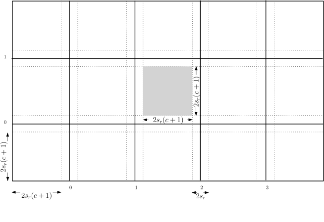
Figure 5: Splitting of $R$ into horizontal and vertical strips

Algorithm 1-COVER-PTAS

1. Initialize the piercing set $P=\emptyset$.

2. Partition the region $R$ by drawing horizontal and vertical strips of width $2s_{r}$ in the interval of $2s_{r}(c+1)$. Let the region $R$ be subdivided into $M\times N$ square blocks after placing the strips. (see Figure 5). The horizontal strips are numbered from bottom to top $(0,1,\ldots M-1)$ and the vertical strips are numbered from left to right $(0,1,\ldots N-1)$.

3. Group the set of the vertical strips into $k(\geq 1)$ disjoint subgroups $(VST_{0},$ $VST_{1},\ldots VST_{k-1})$. Subgroup $VST_{i}$ contains vertical strips whose indices are $(i,i+k,i+2k,\ldots)$.

4. Let $s_{i}$ denote the optimum number of sensors required to cover the line segments that intersect vertical strip $i$.

5. The set of line segments that intersect the vertical strips are also partitioned into $k$ disjoint subsets $(LS_{0},LS_{1},\ldots LS_{k-1})$. All the line segments in $LS_{i}$ must intersect one and only one vertical strip in $VST_{i}$. Hence, the line segments in $LS_{i}$ can be covered optimally using $OPT_{i}=(s_{i}\cup s_{i+k}\cup\ldots)$ sensors.

6. Select a $t$ among $o$ to $k-1$ for which $|OPT_{t}|$ is minimum.

7. Set $P=OPT_{t}$.

8. Remove the set of line segments in $LS_{t}$.

9. The region $R$ is subdivided into small subregions $(R_{1},R_{2},\ldots)$ by the vertical strips in $VST_{t}$.

10. The remaining line segments $L\setminus LS_{t}$ are fully inside these subregions.

11. For each individual disjoint subregion $R_{i}$.

    1. Let $\overline{OPT_{i}}$ denote the minimum number of sensors required to cover the line segments inside $R_{i}$.

    2. $P=P\cup\overline{OPT_{i}}$.

Lemma 6

Let $OPT$ denote the minimum-size set of sensors which covers all the line segments in $L$ then there exists a subgroup $LS_{t}$ which can be covered using at most $\frac{|OPT|}{k}$ sensors.

Proof

Since $OPT$ covers all the line segments in $L$; therefore, it also covers all the line segments in $L_{vs}=(LS_{0}\cup LS_{1}\cup\ldots LS_{k-1})$. As the hippodromes corresponding to the line segments between any two subset $LS_{i}$ and $LS_{j}$ are disjoint where $i$ and $j$ are in between $i=0$ to $(k-1)$ and $i\neq j$. Therefore, $(|OPT_{0}|+|OPT_{1}|+\ldots|OPT_{k-1}|)\leq|OPT|$. Hence, the minimum among $(|OPT_{0}|,|OPT_{1}|,\ldots|OPT_{k-1}|)$ must be at most $\frac{|OPT|}{k}$.

Theorem 7.1

The size of the piercing set $P$ returned by our algorithm is at most $(1+\frac{1}{k})|OPT|$.

Proof

After execution of step(9) of our algorithm the whole region is partitioned into disjoint subregions $(R_{1},R_{2},\ldots)$. Let $(\overline{OPT_{0}},\overline{OPT_{1}},\ldots)$ denote the optimum number of sensors used to cover the line segments which are fully inside each of the individual subregions. The subregions are also separated by the distance $2s_{r}$. Therefore, $(|\overline{OPT_{0}}|+|\overline{OPT_{1}}|+\ldots)\leq|OPT|$. The number of sensors used to cover the line segments that intersect the vertical strips in $LS_{t}$ is at most $\frac{|OPT|}{k}$. Hence, the overall number of sensors used by our algorithm is at most $|OPT|+\frac{|OPT|}{k}=(1+\frac{1}{k})|OPT|$.

Lemma 7

If $B$ is a square region of size $2s_{r}(c+1)\times 2s_{r}(c+1)$ then the number of sensors required to cover all the line segments that are totally inside $B$ is at most $2(c+1)^{2}$. Similarly, the set of line segments that intersect a rectangular strip of size $2s_{r}(c+2)\times 2s_{r}$ can be covered by covering the rectangular strip and it requires at most $\frac{4}{\sqrt{3}}(c+2)$ sensors.

Proof

The maximum size of the square that is inside a circle of radius $s_{r}$ is $\sqrt{2}s_{r}\times\sqrt{2}s_{r}$. Therefore, the number of sensors required to fully cover $B$ is $\frac{4s_{r}^{2}(c+1)^{2}}{2s_{r}^{2}}=2(c+1)^{2}$. There is a rectangle of size $\sqrt{3}s_{r}\times s_{r}$ which is totally inside a circle of radius $s_{r}$. Therefore, the number of sensors used to cover the whole strip is $\frac{2s_{r}(c+2)\times 2s_{r}}{\sqrt{3}s_{r}^{2}}=\frac{4}{\sqrt{3}}(c+2)$.

Lemma 8

The time needed to cover $n_{i}$ line segments inside subregion $R_{i}$ is $O(n_{i}^{\frac{4}{\sqrt{3}}(2Mk-M-k)(c+2)+2Mk(c+1)^{2}})$.

Proof

Let $h$ denote the height of the rectangular region $R$ then the number of rows $M$ of square boxes is $\frac{h}{2s_{r}(c+2)}$. Therefore, the number of boxes in the subregion $R_{i}$ is at most $k*M$. We determine the optimum number of sensors needed to cover all the line segments in each individual box $B_{i,j}$. Let $m_{i,j}$ denote the number of line segments in a box $B_{i,j}$ then the time required to evaluate the optimum number of sensors needed to cover the line segments in $B_{i,j}$ is $O(m_{i,j}^{4(c+1)^{2}})$. Similarly, to cover a set of line segments $T_{i}$ which intersect a vertical strip of size $2s_{r}(c+2)\times 2s_{r}$ can be done in time $O(T_{i}^{\frac{8}{\sqrt{3}}(c+2)})$.
The overall sensors used to cover all the line segments inside $R$ is divided into two sub-parts.
$(i)$ The sensors used to cover line segments optimally inside individual box $B_{i,j}$ where $i\in[0,M-1]$ and $j\in[0,N-1]$.
$(ii)$ The sensors used to cover line segments optimally that intersects the intermediate strips.
In subregion $R_{i}$, there are at most $(k-1)$ vertical strips and $(M-1)$ horizontal strips. Therefore, number of strips of length $2s_{r}(c+2)$ in a subregion $R_{i}$ is at most $(2Mk-M-k)$ and number of boxes in a subregion is at most $Mk$. Hence, the upper bound on the number of sensor needed is $T=\frac{4}{\sqrt{3}}(2Mk-M-k)(c+2)+2Mk(c+1)^{2}$. If there are $n_{i}$ line segments in region $R_{i}$ then the time required to find the optimum number of sensors required to cover the line segments in $R_{i}$ is $n_{i}^{T}$. Therefore, the overall time complexity is $O(n_{i}^{\frac{4}{\sqrt{3}}(2Mk-M-k)(c+2)+2Mk(c+1)^{2}})$.

Lemma 9

The time needed to cover $m_{i}$ line segments that intersect a vertical strips in $VST_{t}$ is $O(m_{i}^{\frac{4}{\sqrt{3}}M(c+2)})$.

Proof

A vertical strip of height $h$ consists of $M$ strips each of height $2s_{r}(c+2)$. Therefore, the upper bound on the number of sensors needed by Lemma 7 is $U=M*\frac{4}{\sqrt{3}}(c+2)$. So, by exhaustive search the time required to cover $m_{i}$ line segments is $O(m_{i}^{\frac{4}{\sqrt{3}}M(c+2)})$.

Theorem 7.2

The overall run time of the algorithm is $O(n^{\frac{4}{\sqrt{3}}(2Mk-M-k)(c+2)+2Mk(c+1)^{2}}+n^{\frac{4}{\sqrt{3}}M(c+2)})$.

Proof

It is comprised of two times $(i)$ The time needed to cover individual subregions optimally and $(ii)$ The time needed to cover the line segments that intersects the vertical strips in $VST_{t}$ optimally. Hence, the total time is $(n_{0}^{T}+n_{1}^{T}+\ldots)+(m_{0}^{U}+m_{1}^{U}+\ldots)\leq n^{T}+n^{U}$ $=O(n^{\frac{4}{\sqrt{3}}(2Mk-M-k)(c+2)+2Mk(c+1)^{2}}+n^{\frac{4}{\sqrt{3}}M(c+2)})$.

8 Discussion and Conclusion

The problem of covering a set of line segments with minimum number of sensors is introduced in this paper. The problem is proved to be NP-hard. We provided a 12-factor approximation algorithm for the special case where the line segments are axis-parallel. We have also shown that a PTAS exists for this problem. These problems are useful in the context of intruder detection in a restricted area. Developing an efficient algorithm with a good approximation factor for the general problem, where the line segments are of arbitrary orientation, and each line segment is covered by at least $k$ sensors. We have also shown a PTAS algorithm for aribitrary oriented line segments for segments whose length are at most some constant times of the sensing range. We would also want to improve the approximation factor of this restricted case (for axis parallel line segments and $k=1$).

References

- [1] A. Agnetis, E.Grandeb, P. B. Mirchandanib, and A. Pacifici. Covering a line segment with variable radius discs. ACM Computers & Operations Research, 36(5):1423–1436, 2009.
- [2] X. Bai, S. Kumar, D. Xuan, Z. Yun, and T. H. Lai. Deploying wireless sensors to achieve both coverage and connectivity. In ACM International Symposium on Mobile Ad Hoc Networking & Computing, pages 131 – 142. Florence, Italy, 2006.
- [3] K. Baumgartner and S. Ferrari. A geometric transversal approach to analyzing track coverage in sensor networks. IEEE Transactions on Computers, 57(8):1–16, 2008.
- [4] M. R. Ceriolia, L. Faria, T. O. Ferreira, and F. Protti. On minimum clique partition and maximum independent set on unit disk graphs and penny graphs: complexity and approximation. Electronic Notes in Discrete Mathematics, 18(1):73–79, 2004.
- [5] G. Chabert and X. Lorca. On the clique partition of rectangle graphs. In Technical report 09-03-INFO. Ecole des Mines de Nantes, 2009.
- [6] T. M. Chan and A.-A. Mahmood. Approximating the piercing number for unit-height rectangles. In CCCG, pages 15–18. Windsor, Ontario, 2005.
- [7] S. Chellappan, B. M. X. Bai, and D. Xuan. Sensor networks deployment using flip-based sensors. In IEEE MASS, pages 291–298. Washington, DC, USA, 2005.
- [8] T. Clouqueur, V. Phipatanasuphorn, P. R., and K. K. Saluja. Sensor deployment strategy for target detection. In WSNA, pages 42–48. Atlanta, Georgia, USA, 2002.
- [9] C. Huang and Y. Tseng. The coverage problem in wireless sensor network. Mobile Network and Applications, 10(4):519–528, 2005.
- [10] S. Kumar, T. H. Lai, and A. Arora. Barrier coverage with wireless sensors. In ACM MOBICOM, pages 284–298. Cologne, Germany, 2005.
- [11] S. Megerian, F. Koushanfar, M. Potkonjak, and M. B. Srivastava. Worst and best-case coverage in sensor networks. IEEE Trans. on Mobile Computing, 4(1):753–763, 2005.
- [12] A. Sekhar, B. S. Manoj, and C. S. R. Murthy. Dynamic coverage maintenance algorithms for sensor networks with limited mobility. In IEEE PERCOM, pages 51–60. Kauai, Hawaii, 2005.
- [13] C. Shen, W. Cheng, X. Liao, and S. Peng. Barrier coverage with mobile sensors. In IEEE ISPAN, pages 99 – 104. Sydney, NSW, Australia, 2008.
- [14] R. Tamassia and I. Tollis. Planar grid embedding in linear time. IEEE Trans. Circuits Systems, 36(9):1230–1234, 1989.
- [15] M. T. Thai, F. Wang, and D. Du. Coverage problems in wireless sensor networks: Designs and analysis. ACM International Journal of Sensor Network, 3(3):191–200, 2008.
- [16] R. Uehara. Np-complete problems on a 3-connected cubic planar graph and their applications. In Technical Report TWCU-M-0004. Tokyo Woman s Christian University, 1996.
- [17] G. Wang, G. Cao, P. Berman, and T. F. L. Porta. Bidding protocols for deploying mobile sensors. IEEE Trans. on Mobile Computing, 6(5):563 – 576, 2007.
- [18] C. Wu, K.C.Lee, and Y. Chung. A delaunay triangulation based method for wireless sensor network deployment. ACM Computer Communications, 30(14-15):2744–2752, 2007.
- [19] G. Xing, X. Wang, Y. Zhang, C. Lu, R. Pless, and C. Gill. Integrated coverage and connectivity configuration for energy conservation in sensor networks. ACM Trans. on Sensor Networks, 1(1):36–72, 2005.
- [20] M. Zhang, X. Du, and K. Nygard. Improving coverage performance in sensor networks by using mobile sensors. In IEEE MILCOM, Atlantic City, pages 3335 – 3341. New Jersey, 2005.