NLTE model atmospheres for the hottest white dwarfs: Spectral analysis of the compact component in nova V4743 Sgr (catalog )

Abstract

Half a year after its outburst in September 2002, nova V4743 Sgr (catalog ) evolved into the brightest supersoft X-ray source in the sky with a flux maximum around 30 Å. We calculated grids of synthetic energy distributions (SEDs) based on NLTE model atmospheres for the analysis of the hottest white dwarfs and present the result of fits to Chandra and XMM-Newton grating X-ray spectra of V4743 Sgr (catalog ) of outstanding quality, exhibiting prominent resonance lines of C V, C VI, N VI, N VII, and O VII in absorption. The nova reached its highest effective temperature ($\mbox{$T_{\mathrm{eff}}$}=740\pm 70\,\mathrm{kK}$) around April 2003 and remained at that temperature at least until September 2003. We conclude that the white dwarf is massive, $\approx 1.1-1.2\,\mathrm{M_{\odot}}$. The nuclear-burning phase lasted for 2 to 2.5 years after the outburst, probably the average duration for a classical nova. The photosphere of V4743 Sgr (catalog ) was strongly carbon deficient ($\approx 0.01$ times solar) and enriched in nitrogen and oxygen ($>5$ times solar). Especially the very low C/N ratio indicates that the material at the white dwarf’s surface underwent thermonuclear burning. Thus, this nova retained some of the accreted material and did not eject all of it in outburst. From March to September 2003, the nitrogen abundance is strongly decreasing, probably new material is already been accreted at this stage.

Key words: stars: abundances – stars: AGB and post-AGB – stars: atmospheres – stars: individual: V4743 Sgr (catalog ) – novae, cataclysmic variables – white dwarfs

1. Introduction

Nova V4743 Sgr (catalog ) (Nova Sgr 2002 c (catalog )) was discovered in outburst in September 2002 and reached $V=5$ mag on 2002 September 20 (Haseda et al., 2002). It was a very fast nova, with a steep decline in the optical light curve and large ejection velocities. The time to decay by 3 mag in the visual (t₃), was 15 days and the FWHM of the H$\alpha$ line reached 2 400 km sec^-1 (Kato et al., 2002). Estimates of the distance from infrared observations vary from $1\,200\pm 300$ pc (Nielbock & Schmidtobreick, 2003) to $\approx 6\,300$ pc (Starrfield & Lyke priv. comm.).

In December 2002, the nova was observed for the first time with Chandra ACIS-S. At that time it was a very soft and moderately luminous X-ray source, with a count rate of about 0.3 cts sec^-1. There were indications that it was not at the peak of X-ray luminosity yet, so a Chandra HRC+LETG observation was done only later, on 2003 March 20. The count rate was astonishingly high, 40 cts sec^-1 during 3.6 hours, then a slow decay, lasting for an hour and a half, was followed by another 1.5 hours of very low luminosity with a measurement of only $\approx 0.02$ cts sec^-1 (Ness et al., 2003; Starrfield et al., 2003). This decline was not due to an eclipse, since the orbital period of the system is $24\,278\pm 259$ sec (or 6.74 hours, Wagner et al., 2003) and no eclipse was observed in a following 10 h XMM-Newton observation two weeks later. An obscuration of a supersoft X-ray source in a nova was observed once before with BeppoSAX, in V382 Vel (catalog ) (Orio et al., 2002). The only reason for this sudden nearly shut down of the source may have been the ejection of a new shell of material that was optically thick to supersoft X-rays from the surface (Orio, 2008). During the Chandra observation in March of 2003 an oscillation with a period of 1 324 sec was detected, with fluctuations of 20% from the mean count rate (see Starrfield et al., 2003; Ness et al., 2003). The most likely cause of this oscillation is a non-radial pulsation of the WD (Starrfield et al., 2003).

A second observation was proposed by us to the XMM-Newton Project Scientist as a target during the Discretionary Time. The nova was observed for 10 h with this satellite on 2003 April 4 (Orio et al., 2003). Three X-ray telescopes with five X-ray detectors were all used: the European Photon Imaging Camera pn (Strüder et al., 2001), two EPIC MOS cameras (Turner et al., 2001), and two Reflection Grating Spectrometers (RGS-1 and RGS-2, Herder et al., 2001). The observation lasted a little over 36 000 sec. The data obtained by the two EPIC MOS cameras suffered from very severe pile up, but the operation of the pn camera was switched to timing mode and yielded a measured average, background corrected EPIC-pn count rate of $1\,348.0\pm 0.3$ cts sec^-1 (Orio et al., 2003), with variations by 40% (Leibowitz et al., 2006). The RGS count rates were about 57 cts sec^-1, and the unabsorbed flux was $1.5\times 10^{-9}$ erg cm^-2 sec^-1, consistent with the flux measured 16 days earlier with Chandra (Leibowitz et al., 2006). Most of the variability is well represented as a combination of oscillations at a set of discrete frequencies lower than 1.7 mHz (Leibowitz et al., 2006). At least five frequencies preserve their coherence over the 16 days time interval between the two observations. The 1 324 sec period detected with Chandra could be split into two periods, of 1 310.1 sec and 1 371.6 sec, both of which are consistent in the Chandra data but it may not have been resolved (Leibowitz et al., 2006). In that article we suggested that a period in the power spectrum of both light curves at the frequency of $\simeq$0.75 mHz (corresponding to 1 371.6 sec) is the spin period of the white dwarf in the system, and that other observed frequencies are signatures of non-radial white dwarf pulsations.

The X-ray evolution was followed with 10 000 sec long exposures with the Chandra LETG in July and September 2003 and in February 2004, and with a 30 000 sec observation with XMM-Newton in September 2004. By this time, the nova X-ray luminosity had decayed by 5 orders of magnitude, but the period of $\approx 1\,370$ sec was still detectable. However, the S/N of the RGS spectra at this epoch was very poor.

We have performed a NLTE spectral analysis of the grating spectra obtained between 2003 March and 2004 February, with NLTE model-atmosphere techniques. The TMAP model-atmosphere code and the construction of the model atoms that are used are described in Sect. 2.1. An attempt to determine photospheric parameters with a XSPEC fit procedure is presented in Sect. 3.1. This is followed by a detailed investigation of the observed, flux-calibrated spectrum of V4743 Sgr (catalog ) (Sect. 3.2). In Sect. 4 we describe how our models fit the Chandra and XMM-Newton observations to interpret the post-nova evolution in the 18 months after the outburst of V4743 Sgr (catalog ).

2. The use of model atmospheres

A previous analysis of Chandra LETG-S observations of V4743 Sgr (catalog ) (Petz et al., 2005), done with the PHOENIX NLTE models with solar abundances, reached $\mbox{$T_{\mathrm{eff}}$}=580\,\mathrm{kK}$. The fit of the model to the data was still poor, and this is not surprising because in the phase directly after the outburst, i.e. when the H burning is still on-going (for years), the surface composition of the WD is poorly known, but it is very unlikely to be solar. With the PHOENIX code, the nova atmosphere is approximated as an expanding, but stationary in time structure. Recently, van Rossum & Ness (2010) presented a new version of PHOENIX that considers mass-loss as well as velocity fields. In the future, such codes will become a powerful tool for the analysis and understanding of novae and other supersoft sources.

However, in order to make progress, we decided to neglect the velocity field, and to use our static NLTE models to investigate basic parameters like $T_{\mathrm{eff}}$  and surface composition. This is not fully justified because especially in the first spectra the lines were significantly blue-shifted, but our aim is at least a qualitative modeling of the XMM-RGS and Chandra-LETG observations done between 2003 March and 2004 February. We started with the highest S/N spectrum, the one obtained with the XMM-Newton RGS gratings on April 4 2003, that we used as a template to adjust the abundances. We then proceeded to fit also the Chandra spectra with the same model, checking whether the abundances we obtained were suitable, and adjusting $T_{\mathrm{eff}}$ for each epoch. In this way, we obtained the evolution of $T_{\mathrm{eff}}$, and the duration of the constant bolometric luminosity phase.

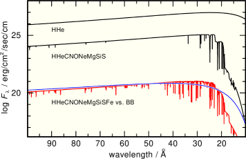
Figure 1.— Comparison of synthetic spectra ($\mbox{$T_{\mathrm{eff}}$}=700\,\mathrm{kK}$, $\log g=9$), from models with different elemental composition (see labels). The abundances are given in Table 3 (model A). For clarity, the HHe and the H-Fe spectra are shifted in $\log F_{\mathrm{\lambda}}$ by $+2$ and $-4$, respectively.

2.1. Model atmospheres and atomic data

For a reliable analysis of X-ray observations of the hottest white dwarfs, detailed NLTE model-atmospheres that consider opacities of all elements from hydrogen up to the iron-group elements (cf. Rauch, 2003) are required. Thus, for our analysis, we employed the plane-parallel, static models calculated with the Tübingen NLTE Model-Atmosphere Package (TMAP, Werner et al., 2003). The construction of model atoms which are used within TMAP follows Rauch & Deetjen (2003). Some details for these extremely hot model atmospheres in the MK-$T_{\mathrm{eff}}$ range are summarized briefly in the following.

Since the surface composition is unknown, we started with the calculation of exploratory H+He+C+N+O models and later included Ne, Mg, Si, S, as well as the iron-group elements. The iron-group elements (Sc – Ni) and Ca are treated with a statistical method (Rauch & Deetjen, 2003) and are represented by one generic model atom.

Beside an element selection, also the construction of the model atoms has to be performed with care. An unrealistic upper cut-off in the number of considered iron-group ionization stages causes an artificial over-population of the highest ionization stage, and thus, affects its lines and the flux level. In Figure 1, the impact of iron-group opacities on the astrophysical flux is demonstrated.

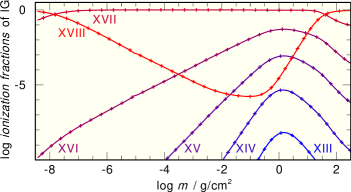
Figure 2.— Ionization fractions of the generic iron-group (IG) model atom in a $\mbox{$T_{\mathrm{eff}}$}=700\,\mathrm{kK}$, $\log g=9$ model. IG XVII is dominant in the line-forming region ($-5.6<\log m<0.5$).

For all values of $T_{\mathrm{eff}}$, the necessary ionization stages of all atoms are determined in advance by test calculations. The selection criterion is, that at least the ion (e.g. in the case of species X), Xⁿ⁺ that is dominant in the line-forming region has to be included together with the neighboring two, i.e. X^(n-1)+ and X⁽ⁿ⁺¹⁾⁺. Thus, the model atoms contain in general three to five ionization stages. E.g. in the case of our generic iron-group model atom, IG XVII is dominant at $\mbox{$T_{\mathrm{eff}}$}=700\,\mathrm{kK}$ and $\log g=9$ [cm sec^-2] (Figure 2). We therefore selected the ionization stages xiv – xviii. Statistics of the model atoms are shown in Table 1. In total, 228 atomic levels are treated in NLTE, 360 additional levels in LTE, and 349 individual line transitions are considered.

Table 1Statistics of the model atoms used in our calculations of the NLTE model atmospheres with $T_{\mathrm{eff}}$ = 0.7 MK. The notation is: N = levels treated in NLTE, L = LTE levels, R = radiative bound-bound transitions. For the generic iron-group (IG) model atom (which represents Ca, Sc, Ti, V, Cr, Mn, Fe, Co, and Ni) the number of individual lines which are combined to so-called superlines is given in brackets.

ion	N	L	R	ion	N	L	R
H I	5	11	10	Ne VII	10	50	12
H II	1	$-$	$-$	Ne VIII	8	18	15
He I	1	25	0	Ne IX	11	9	13
He II	10	22	45	Ne X	1	0	0
He III	1	$-$	$-$	Mg IX	3	23	1
C IV	5	11	6	Mg X	2	3	1
C V	29	21	60	Mg XI	5	6	3
C VI	15	21	26	Mg XII	1	0	0
C VII	1	$-$	$-$	Si X	1	31	0
N V	5	15	6	Si XI	3	23	1
N VI	17	7	33	Si XII	5	4	6
N VII	15	21	30	Si XIII	1	0	0
N VIII	1	$-$	$-$	S XIII	9	21	10
O VI	5	30	6	S XIV	9	1	15
O VII	19	7	32	S XV	1	0	0
O VIII	15	30	30	IG XIV	6	0	20	(21757)
O IX	1	$-$	$-$	IG XV	6	0	20	(4794)
				IG XVI	5	0	14	(184)
				IG XVII	4	0	9	(3409)
				IG XVIII	1	0	0

3. Spectral analysis

A first grid of models is composed of H+He+C+N+O with solar abundance ratios (Asplund et al., 2009) within $\mbox{$T_{\mathrm{eff}}$}=0.45-1.05\,\mathrm{MK}$ and a fixed surface gravity of $\log g=9$ (Figure 3). We note that all synthetic energy distributions (SEDs) in our model grids described here are available at in Virtual Observatory (VO) compliant form from the VO service TheoSSA provided by the German Astrophysical Virtual Observatory (GAVO) as well as atables for the use with XSPEC.

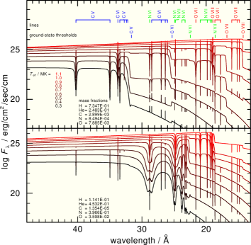
Figure 3.— Comparison of NLTE model fluxes (H+He+C+N+O, solar abundances, top panel) at different $T_{\mathrm{eff}}$. The wavelength interval corresponds to $0.95-0.26$ keV. The positions of C, N, and O lines (at top) and bound-free absorption thresholds are marked. In the bottom panel, the abundance ratios are taken from nova models of Prialnik (priv. comm.) except for the carbon abundance which is reduced by a factor of 100.

3.1. Preliminary analysis

We started with the XMM-Newton RGS spectra of 2003 April (Table 2). The data were reduced with the ESA XMM-Newton Science Analysis System (SAS) software, version 5.3.3, using the latest calibration files available. The RGS dispersion gratings cover the $5-35$ Å wavelength range ($2.48-0.35$ keV), although we obtained useful signal only in the $5-26$ Å range ($2.48-0.48$ keV). The RGS data are piled-up, but in a dispersion instrument, piled-up events at a discrete wavelength increase in pulse height amplitude by an integer multiple of the intrinsic energy. Furthermore, since the softness of the source precludes any intrinsic photons from higher spectral orders, we can confidently identify events that occur within the higher order spectral masks for an on-axis point source as piled-up first order photons. This is verified by line matching of the piled-up events using the first order response matrix. Source events dominate over background and scattered source light in the first three orders. Consequently we added events within the second and third order extraction masks to the first order events, thus reclaiming the piled-up events and increasing the signal-to-noise of the spectra.

Table 2X-ray observations of V4743 Sgr used in the analysis.

				exp. time
satellite	instrument	ObsId	Obs date (start)
				sec
Chandra	HRC+LETG	3775	2003-03-19 09:30:12	27058
XMM-Newton	RGS-1	0127720501	2003-04-04 22:24:12	35215
XMM-Newton	RGS-2	0127720501	2003-04-04 22:24:12	35214
Chandra	HRC+LETG	3776	2003-07-18 21:35:29	13746
Chandra	HRC+LETG	4435	2003-09-25 23:51:50	14378
Chandra	HRC+LETG	5292	2004-02-28 01:07:42	13530

In a first step, we compared our SEDs with the XMM-Newton observation of V4743 Sgr (catalog ) via XSPEC. We let the neutral hydrogen column density $N_{\mathrm{H\,I}}$ [cm^-2] and $T_{\mathrm{eff}}$ vary as free parameters in XSPEC. XSPEC determines $\mbox{$T_{\mathrm{eff}}$}=709\,\mathrm{kK}$ and $\log N_{\mathrm{H\,I}}=20.58$. In Figure 4 (top panel), we show this XSPEC fit. The reader may miss the typical XSPEC residuals at the bottom of the plots. Since our models do not include all the elements with all the lines that may be exhibited in the observation, the residuals are not that helpful like in comparisons of simple models where continuum slope and a handful of strategic lines has to be reproduced. Thus, we decided to omit the residual plots generally. Instead, the reader should judge the strengths of prominent lines and absorption edges with respect to the (estimated) local flux continuum.

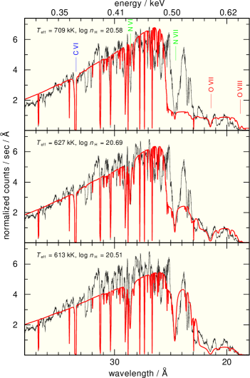
Figure 4.— Comparison of the XMM-Newton RGS-1 observation of V4743 Sgr (catalog )  (Table 2) with NLTE model-atmosphere fluxes (H+He+C+N+O models with solar abundances, but different carbon abundances: top: [C] = 0.0, middle: [C] = $-$1.0, bottom: [C] = $-$2.0). $T_{\mathrm{eff}}$ and $N_{\mathrm{H}}$ are determined with XSPEC. The SEDs are shifted by $-1\,800\,\mathrm{km/sec}$ in order to match the observed position of the N VII resonance line. The positions of resonance lines of C VI, N VI, N VII, O VII, and O VIII are marked.

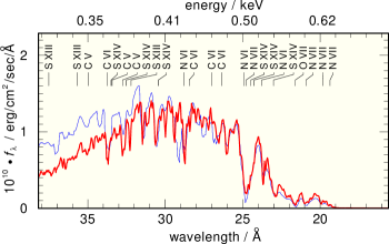
Figure 5.— Comparison of the RGS fluxed spectrum of V4743 Sgr (catalog ) obtained from the XMM-Newton pipeline (thick line) with the absolute flux calculated by XSPEC (thin line, see text for details). The XSPEC spectrum is convolved with a Gaussian of 0.10 Å (FWHM) in order to match the resolution of the binned RGS fluxed spectrum. Note that both spectra agree well for $\lambda\raisebox{-1.00006pt}{$\stackrel{{\scriptstyle<}}{{{\mbox{\tiny$\sim$}}}}$}32$ Å. The marks indicate positions of lines that are included in our models.

As expected, a solar composition does not well represent the white dwarf spectrum in V4743 Sgr (catalog ). The flux at wavelengths smaller than 26 Å is far too low. In test calculations, we decreased the carbon abundance to [C] = $-$1.0 ([X] denotes log [mass fraction / solar mass fraction] of species X) and to [C] = $-$2.0. We achieved a much better fit at [C] = $-$2.0, $\mbox{$T_{\mathrm{eff}}$}=610\,\mathrm{kK}$, and $\log N_{\mathrm{H\,I}}=20.54$ for $\lambda<26$ Å (Figure 4).

We wondered whether the small wavelength interval ($18-38$ Å) of our XMM-Newton RGS spectra leads in the XSPEC fit procedure to a smaller $N_{\mathrm{H\,I}}$ than found by Petz et al. (2005, $\log N_{\mathrm{H\,I}}=21.60$, $\mbox{$T_{\mathrm{eff}}$}=580\,\mathrm{kK}$) obtained fitting the a Chandra LETG spectrum ($18-58$ Å). In Sect. 4 we show however, that we fitted the Chandra LETG spectrum of March 19, 2003 and used the same wavelength range as Petz et al. (2005), deriving $\mbox{$T_{\mathrm{eff}}$}=601\,\mathrm{kK}$ and $\log N_{\mathrm{H\,I}}=20.95$ for the [C] = $-$2.0 model. A decreasing N${}_{\mathrm{H\,I}}$ from March to April is consistent with intrinsic absorption of the ejecta clearing up.

3.2. Spectral analysis of the flux-calibrated spectrum

Before we start now with a detailed analysis, we mention that the calibration of the instruments that were used to obtain our data is still an issue. Different calibration products (response matrices and effective areas) may play an important role on the results obtained from fits to X-ray spectra. Cross calibration between instruments has improved over the years (see, e.g. Beuermann et al., 2006, 2008) but there is yet room for further improvement.

While the wavelength scale of X-ray gratings instruments is generally very well known, the effective areas of these instruments are less well calibrated. For example, a comparison between the continuum calibrations of the gratings and CCD instruments on board XMM-Newton by Stuhlinger et al. (2008) shows deviations between the RGS and the EPIC-pn of 3 % above 0.5 keV and about 10 % below that energy. While not negligible, these deviations are still smaller than the deviations between data and model caused by simplifications in the atmosphere modeling, and can therefore be ignored.

The preliminary analysis presented in the last section shows clearly that the carbon abundance in V4743 Sgr (catalog ) is strongly subsolar. The determination of $T_{\mathrm{eff}}$ and a more precise abundance determination is hampered by the complex XSPEC fitting procedure and the necessity to calculate extended grids of models with different $T_{\mathrm{eff}}$ if the abundances are changed. The latter results in unreasonable computational times.

A more straightforward approach is to use the flux-calibrated spectra instead of count-rate spectra. However, these spectra contain uncertainties in the flux. We tried to calibrate the RGS spectra of V4743 Sgr (catalog ) in two different ways. One way is by making use of the provided XMM-SAS pipeline products, the so called “fluxed” spectra. Such spectra are e.g. shown by BiRD, the Browsing Interface for RGS Data, with the purpose of visualizing the data free from the peculiarities of the instrument. However, RGS fluxed spectra are computed in the pipeline by dividing the extracted spectrum by the effective area calculated from its corresponding response matrix. This procedure neglects the redistribution of monochromatic response into the dispersion channels, and therefore these spectra should not be used for very detailed analysis. The second version of the flux-calibrated spectrum is calculated by XSPEC and is not independent from the models which are used within the XSPEC fit procedure (Figure 5).

We are aware of these uncertainties, but with the aim to determine $T_{\mathrm{eff}}$ within an error range of about 10 % and element abundances within 0.5 dex, we used the flux-calibrated spectra. We calculated synthetic profiles of the resonance lines of the two highest ionization stages of C, N, and O (Figure 6). These appear to be strongly dependent of $T_{\mathrm{eff}}$ within the parameter range of our grids.

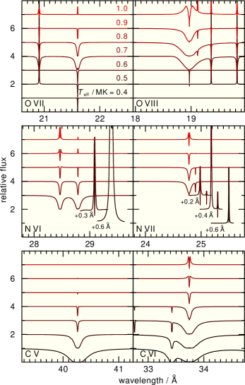
Figure 6.— Synthetic profiles of the O VII, O VIII, N VI, N VII, C V, and C VI resonance lines, calculated from H+He+C+N+O model atmospheres with $T_{\mathrm{eff}}$ = 0.4 – 1.0 MK, $\log g=9$ and solar abundances. The nitrogen lines of the cooler models that appear in emission are shifted for clarity.

The best XSPEC fit of the [C] = $-$2.0 model yields $\mbox{$T_{\mathrm{eff}}$}=610\,\mathrm{kK}$. Since the maximum flux level is not well reproduced by this fit (Figure 4), we estimate that $T_{\mathrm{eff}}$ of V4743 Sgr (catalog ) may be slightly higher. Thus, we selected models with $\mbox{$T_{\mathrm{eff}}$}=600-800\,\mathrm{kK}$ and model-A abundances (Table 3) for a comparison with the RGS fluxed spectrum (Figure 7). The flux level below $\stackrel{{\scriptstyle<}}{{{\mbox{\tiny$\sim$}}}}$ 30 Å is strongly dependent on $T_{\mathrm{eff}}$ and at first glance, we can achieve good agreement with the RGS flux level at $\mbox{$T_{\mathrm{eff}}$}=700\,\mathrm{kK}$ and $\log N_{\mathrm{H\,I}}$ = 20.90. Moreover, the prominent absorption lines N VI $\lambda\lambda\,28.79,24.90,23.77$ Å, N VII $\lambda\lambda\,24.78,20.91,19.82,19.32$ Å, and O VII $\lambda\,21.60$ Å are well reproduced by our model. A detailed inspection of the O VIII $\lambda\,18.96$ Å resonance line shows that the observed continuum flux on its high-energy wing is much lower than in the synthetic spectrum. A stronger N VII bound-free ground-state absorption edge (18.59 Å) could probably decrease this flux. Consequently, we increased the nitrogen abundance in the following models.

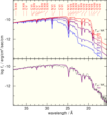
Figure 7.— Top: SEDs of our model with [C] = $-$2.0 and $\mbox{$T_{\mathrm{eff}}$}=600-800\,\mathrm{kK}$. They are normalized to the $\mbox{$T_{\mathrm{eff}}$}=700\,\mathrm{kK}$ flux level at 38 Å for this comparison. The positions of lines are marked. Bottom: Comparison of the synthetic spectra of our [C] = $-$2.0, $\mbox{$T_{\mathrm{eff}}$}=700\,\mathrm{kK}$ model with the RGS fluxed spectrum of V4743 Sgr (catalog ).

In Figure 7 the $T_{\mathrm{eff}}$-dependency of the strengths of prominent bound-free absorption edges (for an identification, see Figure 9) is shown. Especially, the N VI and N VII ground-state edges at 22.46 Å and 18.59 Å, respectively, appear very sensitive on $T_{\mathrm{eff}}$. In order to improve the fit, we performed some fine-tuning of the abundances (cf. Table 3, model B). E.g. in the case of sulfur, model A (Table 3) yields a much too strong S XIV line at 32.51 Å, i.e. the sulfur abundance is too high in the relevant $T_{\mathrm{eff}}$ range. In the case of nitrogen, we find prominent absorption edges as well as absorption lines in the observation which are suitable to adjust the abundance. In the case of other species, it is difficult to determine their abundances precisely because they do not exhibit significant features in the XMM-Newton observation. However, this can be used to determine at least upper abundance limits. Figure 8 demonstrates how the SEDs change if the abundance of one particular element is artificially increased by a factor of ten. We note that only nitrogen, oxygen, silicon, and the iron-group elements have an influence on the flux in the RGS wavelength range if their abundances are increased.

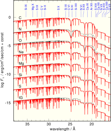
Figure 8.— Comparisons of the SED of our $\mbox{$T_{\mathrm{eff}}$}=750\,\mathrm{kK}$ model B (thin line, Table 3) to SEDs of models where the abundance of one element (indicated by labels) is increased by a factor of ten. The positions of ground-state absorption edges are marked at the top.

We compared the strengths of the N VI and N VII edges in our models with the observation (Figure 9). With these models (Table 3, model B), we achieve the best fit at $\mbox{$T_{\mathrm{eff}}$}=740\,\mathrm{kK}$ and $\log N_{\mathrm{H\,I}}=20.85$.

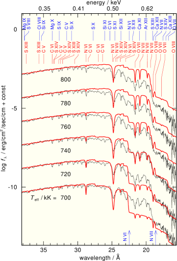
Figure 9.— Dependance of the strengths of the N VI and N VII ground-state thresholds (positions marked by the arrows) on $T_{\mathrm{eff}}$. The SEDs are compared with the RGS fluxed spectrum of V4743 Sgr (catalog ) and normalized to match the flux at 38 Å. The SEDs were convolved with a Gaussian of 0.10 Å (FWHM). Positions of ground-state thresholds are marked at top, of those line transitions just below that marks.

Table 3Element abundances in our models given in [X] = log [mass fraction / solar mass fraction] of species X. Solar abundances are taken from Asplund et al. (2009). We note that in model B, the abundances for Ne, Mg, S, and IG (Ca – Ni) are determined upper limits. An error range of $\pm 0.3\,\mathrm{dex}$ is estimated from detailed comparison with the observations.

element	model A		model B
H	-0.	573	-0.	688
He	0.	497	0.	382
C	-2.	614	-1.	513
N	0.	386	1.	803
O	0.	425	1.	528
Ne	-0.	333	-0.	474
Mg	0.	000	-0.	454
Si	0.	000	0.	167
S	0.	000	-1.	583
IG	0.	000	0.	828

In Figure 10, we show a comparison of TMAP SEDs with the flux-calibrated Chandra spectra from 2003. In 2004, the measured flux level and thus, $T_{\mathrm{eff}}$ are much lower and we disregard that observation here. Furthermore, for reasons of simplicity, we used a $\mbox{$T_{\mathrm{eff}}$}=720\,\mathrm{kK}$ model with model-B abundances (Table 3) and varied only the C and N abundances in order to improve the fit. The observed strengths of the N vi and N vii resonance lines as well as their ground-state edges are well reproduced for all observations. Since the N vi / N vii ionization balance is very sensitive to $T_{\mathrm{eff}}$ (Figure 6), $\mbox{$T_{\mathrm{eff}}$}=720\,\mathrm{kK}$ appears a good estimate. Our model fits show that the N abundance is decreasing from March to September by a factor of about ten. The C lines, e.g. at about 34 Å are well matched in September while they appear too weak in March and July. A higher C abundance would result in the appearance of a strong C vi ground-state absorption edge at 25.3 Å that is not visible in the observation.

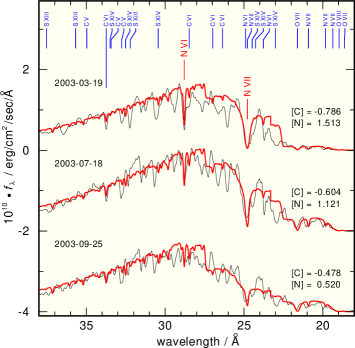
Figure 10.— Comparison of flux-calibrated Chandra observations of V4743 Sgr (catalog )  (Table 2) with our SEDs ($\mbox{$T_{\mathrm{eff}}$}=720\,\mathrm{kK}$, $\log g=9.0$). All abundances, but for C and N, are from model-grid B (Table 3). For clarity, the July and September observations are shifted in $f_{\lambda}$ by $-2\cdot 10^{10}$ and $-4\cdot 10^{10}\,\mathrm{erg/cm^{2}/sec/\AA}$, respectively .

In a last step, we used the SEDs of our model-A and model-B grids (Table 3) for a comparison with the XMM-Newton observation with XSPEC (Figure 11). The differences in the SEDs of the best fitting models A and B are small. If we assume the mean $T_{\mathrm{eff}}$, we are able to constrain the $T_{\mathrm{eff}}$ range of V4743 Sgr (catalog ) to $\mbox{$T_{\mathrm{eff}}$}=740\pm 70\,\mathrm{kK}$. The deviations of the abundance of both models (Table 3) show the difficulty of a precise abundance determination if only a few spectral lines are available for the analysis.

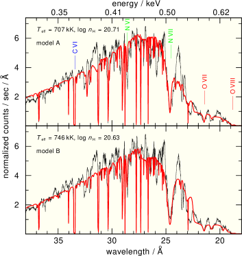
Figure 11.— Comparison of the XMM-Newton RGS-1 observation of V4743 Sgr (catalog )  (Table 2) with our best fitting SEDs from model grids A and B (Table 3). $T_{\mathrm{eff}}$ and $\log N_{\mathrm{H}}$ were determined with XSPEC.

4. The spectral evolution of V4743 Sgr

We then proceeded to fit the Chandra LETG spectra at three different epochs using the same models. The LETG spectra were reduced using the CIAO software, version 4.1.1.

In the first 18 months after the outburst of V4743 Sgr (catalog ), Chandra LETG spectra were obtained roughly every three months (Table 2). These observations allow an investigation on the spectral evolution, e.g. on the change of its $T_{\mathrm{eff}}$. In Figure 12, we compare the observations with SEDs of our grid (models B). No individual fine-tuning of the model abundances for the different spectra was performed. Although this might improve the fit, we estimate that the impact on the determined $T_{\mathrm{eff}}$ is small.

The Chandra observations (energy range $0.22-0.69$ keV) show that V4743 Sgr (catalog ) was at a maximum of $T_{\mathrm{eff}}$ ($\approx 700$ kK) for about one year, then $T_{\mathrm{eff}}$ appears to decrease by about 10 % in the following six months (Figure 12, left panel).

In order to judge the quality of our spectral analysis of the Apr 2004 XMM-Newton observation that covers a smaller energy range ($0.32-0.69$ keV), we restricted the fit range of XSPEC (Figure 12, right panel) for the Chandra observations. With this restriction, the determined $T_{\mathrm{eff}}$ is in general higher and the interstellar neutral hydrogen density is smaller, but the deviations are within our expected error range of about 10 %.

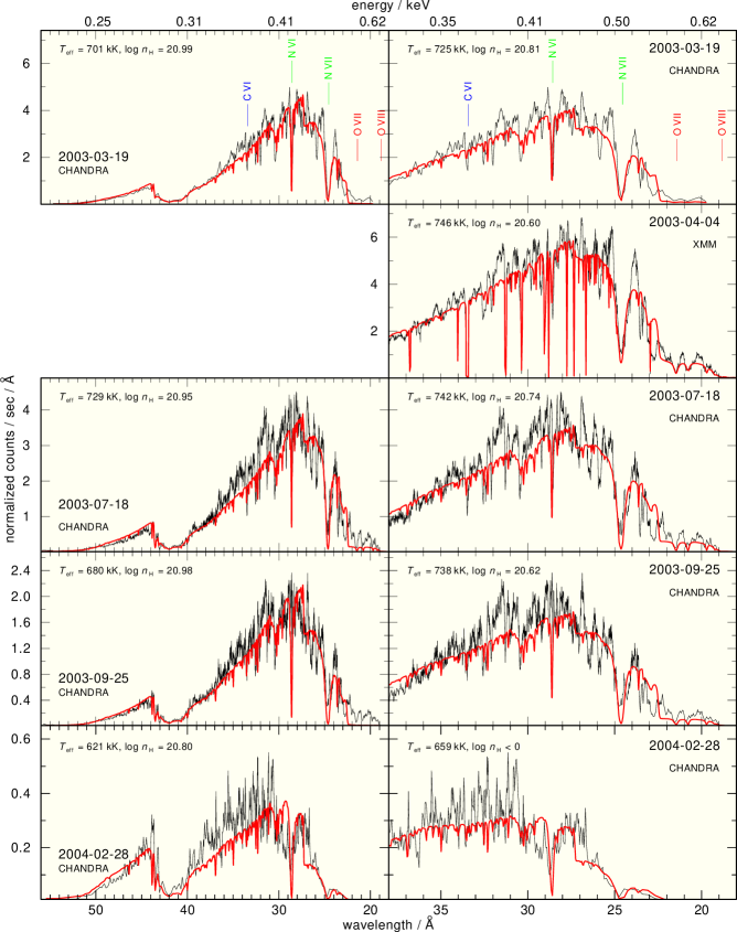
Figure 12.— Comparison of Chandra and XMM-Newton observations of V4743 Sgr (catalog ) (Table 2) with our SEDs from model grid B (Table 3). $\log N_{\mathrm{H}}$ and $T_{\mathrm{eff}}$ were determined with XSPEC. The fit range was restricted to $18-56$ Å ($0.22-0.69$ keV, left panel) and $18-38$ Å ($0.32-0.69$ keV, right panel) to represent the Chandra and XMM-Newton wavelength ranges, respectively.

5. Results and conclusions

We have calculated NLTE model atmospheres including opacities of the elements H, He, C, N, O, Ne, Mg, Si, S, and Ca – Ni and fitted XMM-Newton RGS spectra and Chandra LETG spectra of V4743 Sgr (catalog ).

The fit to the RGS spectra (Table 2) based on these models (Table 3) is best at a $T_{\mathrm{eff}}$ of about $740\pm 70$ kK, $\log g=9$, and $\log N_{\mathrm{H}}=20.7\pm 0.3$. Although this fit is not perfect and there are uncertainties in the so-called RGS fluxed spectrum used for our spectral analysis, the overall flux distribution as well as prominent line features are well in agreement with the observation (Figure 11). The photospheric abundances have been adjusted and we can give at least upper limits for N, O, Si, and Ca – Ni (Figure 8). The determined C/N ratio is very low (Table 3), indicating that the material on the white dwarf surface has been processed through thermonuclear burning. We expect that freshly accreted material after the outburst or dredged-up material from the white dwarf interior, would have a very different range of abundances and suggest this is a proof that the white dwarf is retaining some accreted material after each outburst. This may imply that V4743 Sgr (catalog ) is on a track towards supernova Ia explosion, although it retains after each outburst only just enough material to burn in less than 2.5 years.

The fit to the Chandra LETG grating spectra shows that V4743 Sgr (catalog ) reached its highest temperature around April 2003 and remained at that temperature at least until September 2003. The duration of the constant bolometric luminosity phase at constant $T_{\mathrm{eff}}$ was between 2 and 2.5 years, probably the average for a classical nova (e.g., Orio et al., 2001). In Shara et al. (1979), $T_{\mathrm{eff}}$ of the constant bolometric luminosity phase is 780 000 K for a $1.25\,\mathrm{M_{\odot}}$ WD. $T_{\mathrm{eff}}$ of the calculations is not always published in papers on nova-outburst models (cf. Kovetz & Prialnik, 1994; Prialnik & Kovetz, 1995), but published values range from 460 000 K for a $0.8\,\mathrm{M_{\odot}}$ (Shara et al., 1979) to an extreme 2 500 000 K for a $1.4\,\mathrm{M_{\odot}}$ WD accreting at very high rate. The value of $T_{\mathrm{eff}}$ is dependent on mass-accretion rate, on the chemical composition and on the WD temperature at the onset of hydrogen burning, but generally a value of about 700 000 K is only reached for $M>1.1\,\mathrm{M_{\odot}}$ (Prialnik 2009, priv. comm.). To summarize, the peak $T_{\mathrm{eff}}$ of about 740 kK indicates that the WD is very massive, with $\approx 1.1-1.2\,\mathrm{M_{\odot}}$.

To explain the apparently decreased nitrogen abundance in the months after the outburst (Figure 10), we conjecture that probably new material is already been accreted at this stage, while CNO burning at the bottom of the envelope is already proceeding at a lower rate before turn-off.

A crucial point for the understanding of processes during the nova outburst may be the time-dependent prediction of surface abundances as well as the spectral analysis of high-resolution X-ray spectra taken from outburst to the end of surface H burning. The inspection of available Chandra and XMM-Newton observations of V4743 Sgr (catalog ), taken in the 18 months after the outburst has shown that obtaining new X-ray grating spectra of future novae every week is highly desirable.

In applications to novae, TMAP still lacks some physics, most notably the velocity fields. Although TMAP is not especially designed for the calculation of SEDs at extreme photospheric parameters, it is a flexible and robust tool for the determination of basic parameters like $T_{\mathrm{eff}}$ for line identifications (cf. Rauch et al., 2008), and to derive a reliable range of abundances in the white-dwarf atmosphere.

Acknowledgements.

TR is supported by the German Aerospace Center (DLR) under grant 05 OR 0806. This research has made use of the SIMBAD database, operated at CDS, Strasbourg, France. MO is supported by Chandra-Smithsonian and XMM-Newton NASA grants for the data analysis. This research has made use of software provided by the Chandra X-ray Center (CXC) in the application packages CIAO, ChIPS, and Sherpa.

References

- Asplund et al. (2009) Asplund, M., Grevesse, N., Sauval, A. J., & Scott, P. 2009, ARAA, 47, 481
- Beuermann et al. (2006) Beuermann, K., Burwitz, V., & Rauch, T. 2006, A&A, 458, 541
- Beuermann et al. (2008) Beuermann, K., Burwitz, V., & Rauch, T. 2008, A&A, 481, 769
- Haseda et al. (2002) Haseda, K., West, D., Yamaoka, H., & Masi, G. 2002, IAU Circ., 7975
- Herder et al. (2001) den Herder, J. W., Brinkman, A. C., Kahn, S. M., et al. 2001, A&A, 365, L 7
- Kato et al. (2002) Kato, T., Hishikura, T., West, J. D., et al. 2002, IAU Circ., 7976
- Kovetz & Prialnik (1994) Kovetz, A., & Prialnik, D. 1994, ApJ, 424, 319
- Leibowitz et al. (2006) Leibowitz, E., Orio, M., Gonzalez-Riestra, R., et al. 2006, MNRAS, 371, L 424
- Ness et al. (2003) Ness, J.-U., Starrfield, S., Burwitz, V., et al. 2003, ApJ, 594, L 127
- Nielbock & Schmidtobreick (2003) Nielbock, M., & Schmidtobreick, L. 2003, A&A, 400, L 5
-
Orio (2008)
Orio, M.
2008,
in: The X-ray Universe 2008,
http://xmm.esac.esa.int/external/xmm_science/workshops/2008symposium - Orio et al. (2001) Orio, M., Covington, J., & Ögelman, H. 2001, A&A, 373, 542
- Orio et al. (2002) Orio, M., Parmar, A., Greiner, J., Ögelman, H., Starrfield, S., & Trussoni, E. 2002, MNRAS, 333, L 11
- Orio et al. (2003) Orio, M., Leibowitz, E., Rodriguez, P., et al. 2003, IAU Circ., 8131
- Petz et al. (2005) Petz, A., Hauschildt, P. H., Ness, J.-U., & Starrfield, S. 2005, A&A, 431, 321
- Prialnik & Kovetz (1995) Prialnik, D., & Kovetz, A. 1995, ApJ, 445, 789
- Rauch (1997) Rauch, T. 1997, A&A, 320, 237
- Rauch (2003) Rauch, T. 2003, A&A, 403, 709
- Rauch & Deetjen (2003) Rauch, T., & Deetjen, J. L. 2003, in: Workshop on Stellar Atmosphere Modeling, eds. I. Hubeny, D. Mihalas, K. Werner, The ASP Conference Series (San Francisco: ASP), 288, 103
- Rauch et al. (2005) Rauch, T., Orio, M., Gonzales-Riestra, C., & Still, M. 2005, in: White Dwarfs, eds. D. Koester, S. Moehler, The ASP Conference Series (San Francisco: ASP), 334, 423
- Rauch et al. (2008) Rauch, T., Suleimanov, V., Werner, K. 2008, A&A, 490, 1127
- Shara et al. (1979) Shara, M. M., Prialnik, D., Shaviv, G. 1979, A&A, 72, 192
- Starrfield et al. (2003) Starrfield, S., Drake, J. J., Ness, J.-U., & Orio, M. 2003, IAU Circ., 8107
- Strüder et al. (2001) Strüder, L., Briel, U., Dennerl, K., et al. 2001, A&A, 365, L 18
- Stuhlinger et al. (2008) Stuhlinger, M., Kirsch, M. G. F., Santos-Lleo, M., et al. 2008, XMM-SOC-CAL-TN-0052 Issue 5.0
- Turner et al. (2001) Turner, M. J. L., Abbey, A., Arnaud, M., et al. 2001, A&A, 365, L 27
- van Rossum & Ness (2010) van Rossum, D. R., & Ness, J.-U. 2010, AN, 331, 75
- Wagner et al. (2003) Wagner, R. M., et al. 2003, IAU Circ., 8176
- Werner et al. (2003) Werner, K., Dreizler, S., Deetjen, J. L., Nagel, T., Rauch, T., & Schuh, S. L. 2003, in: Workshop on Stellar Atmosphere Modeling, eds. I. Hubeny, D. Mihalas, K. Werner, The ASP Conference Series (San Francisco: ASP), 288, 31