Modelling and Numerical Simulation of gas migration in a nuclear waste repository

Abstract

We present a compositional compressible two-phase, liquid and gas, flow model for numerical simulations of hydrogen migration in deep geological radioactive waste repository. This model includes capillary effects and the gas diffusivity. The choice of the main variables in this model, Total or Dissolved Hydrogen Mass Concentration and Liquid Pressure, leads to a unique and consistent formulation of the gas phase appearance and disappearance. After introducing this model, we show computational evidences of its adequacy to simulate gas phase appearance and disappearance in different situations typical of underground radioactive waste repository.

Keywords: Two-phase flow, compositional flow, porous medium, underground nuclear waste management

1 Introduction

The simultaneous flow of immiscible fluids in porous media occurs in a wide variety of applications. The most concentrated research in the field of multiphase flows over the past four decades has focused on unsaturated groundwater flows, and flows in underground petroleum reservoirs. Most recently, multiphase flows have generated serious interest among engineers concerned with deep geological repository for radioactive waste. There is growing awareness that the effect of hydrogen gas generation, due to anaerobic corrosion of the steel engineered barriers of radioactive waste packages(carbon steel overpacks and stainless steel envelopes), can affect all the functions allocated to the canisters or to the buffers and the backfill. The host rock safety function may even be threaten by overpressurisation leading to opening fractures in the host rock and inducing groundwater flow and transport of radionuclides outside of the waste site boundaries.

Equations governing this type of flow in porous media are inherently nonlinear, and the geometries and material properties characterizing many situations in many applications ( petroleum reservoir, gas storage, waste repository), can be quite irregular and contrasted. As a result of all these difficulties, numerical simulation often offers the only viable approach to modelling multiphase porous-media flows . In nuclear waste management, the migration of gas through the near field environment and the host rock, involves two components, water and pure hydrogen $\text{H}_{2}$; and two phases ”liquid” and ”gas”. Our ability to understand and predict underground gas migration is crucial to the design and to assessing the performance of reliable nuclear waste storages. This is a fairly new frontier in multiphase porous-media flows, and again the inherent complexity of the physics leads to governing equations for which the only practical way to produce solutions may be numerical simulation.

This paper addresses one of the outstanding physical and mathematical problems in multiphase flow simulation: the appearance and disappearance of one of the phases, leading to the degeneracy of the equations satisfied by the saturation. In order to overcome this difficulty, we discuss a formulation based on variables which doesn’t degenerate and hence could be used as an unique formulation for both situations, liquid saturated and unsaturated. We will demonstrate through four numerical tests, the ability of this new formulation to actually cope with the appearance or/and disappearance of one phase in simple, typical but challenging situations, like the ones we met in underground radioactive waste repository simulations.

2 Modeling Physical Assumptions

We consider herein a porous medium saturated with a fluid composed of 2 phases, liquid and gas, and two components. According to the application we have in mind, we consider the fluid as a mixture of two components: water (only liquid) and hydrogen ($\text{H}_{2}$, mostly gas) or any gas with similar thermodynamical properties. In the following, for sake of simplicity we will call hydrogen the non-water component and use indices $w$ and $h$ for the water and the hydrogen components.

We neglect the water vaporization since, in underground formations with high water pressure, the water vapor does not contribute significantly to the gas phase pressure . The water component is incompressible while the gas phase follow the ideal gas law. The whole fluid system is in thermal equilibrium and the porous medium is rigid, meaning that the porosity $\Phi$ is only a function of the space variable $\Phi=\Phi(\mbox{\bf x})$; moreover, since hydrogen is highly diffusive we include the dissolved hydrogen diffusion in the liquid phase .

The two phases are denoted by indices, $l$ for liquid, and $g$ for gas. Associated to each phase $\alpha\in\{l,g\}$, we have, in the porous medium, the phase pressures $p_{\alpha}$, the phase saturations $S_{\alpha}$, the phase mass densities $\rho_{\alpha}$ and the phase volumetric flow rates $\mathbf{q}_{\alpha}$. The phase volumetric flow rates are given by the Darcy-Muskat law:

$$\mbox{$\mathbf{q}_{l}$}=-\mathbb{K}(\mbox{\bf x})\lambda_{l}(S_{l})\left(\mbox{$\nabla$}p_{l}-\rho_{l}\mbox{$\mathbf{g}$}\right),\quad\mbox{$\mathbf{q}_{g}$}=-\mathbb{K}(\mbox{\bf x})\lambda_{g}(S_{g})\left(\mbox{$\nabla$}p_{g}-\rho_{g}\mbox{$\mathbf{g}$}\right),$$ (1)

where $\mathbb{K}(\mbox{\bf x})$ is the absolute permeability tensor, $\lambda_{\alpha}(S_{\alpha})$ is the $\alpha-$phase relative mobility function, and $\mathbf{g}$ is the gravity acceleration; $S_{\alpha}$ is the reduced $\alpha-$phase saturation and then satisfies:

$$S_{l}+S_{g}=1.$$ (2)

Pressures are connected through a given capillary pressure law:

$$p_{c}(S_{g})=p_{g}-p_{l}.$$ (3)

From definition (3) we notice that $p_{c}$ is a strictly increasing function of gas saturation, $p_{c}^{\prime}(S_{g})>0$, leading to a capillary constraint:

$$p_{g}>p_{l}+p_{c}(0),$$ (4)

where $p_{c}(0)\geq 0$ is the capillary curve entry pressure ( see Figure 2).

Since the liquid phase could be composed of water and dissolved hydrogen, we need to introduce the water mass concentration $\rho_{l}^{w}$ in the liquid phase, and the hydrogen mass concentration $\rho_{l}^{h}$ in the liquid phase. Note that the upper index is the component index, and the lower one denotes the phase. We have, then

$$\rho_{l}=\rho_{l}^{w}+\rho_{l}^{h}.$$ (5)

As said before, in the gas phase, we neglect the water vaporization and we use the ideal gas law:

$$\rho_{g}=C_{v}p_{g},$$ (6)

with $C_{v}=M^{h}/(RT)$, where $T$ is the temperature, $R$ the universal gas constant and $M^{h}$ the hydrogen molar mass. Mass conservation for each component leads to the following differential equations:

$$\Phi\frac{\partial}{\partial t}\left(S_{l}\rho_{l}^{w}\right)+\mbox{$\mbox{div}$}\left(\rho_{l}^{w}\mbox{$\mathbf{q}_{l}$}+\mbox{$\mathbf{j}_{l}^{w}$}\right)={\cal F}^{w},$$ (7)

$$\Phi\frac{\partial}{\partial t}\left(S_{l}\rho_{l}^{h}+S_{g}\rho_{g}\right)+\mbox{$\mbox{div}$}\left(\rho_{l}^{h}\mbox{$\mathbf{q}_{l}$}+\rho_{g}\mbox{$\mathbf{q}_{g}$}+\mbox{$\mathbf{j}_{l}^{h}$}\right)={\cal F}^{h},$$ (8)

where the phase flow velocities, $\mathbf{q}_{l}$ and $\mathbf{q}_{g}$, are given by the Darcy-Muskat law (1), ${\cal F}^{c}$ are the source terms, and $\mathbf{j}_{l}^{c}$, $c\in\{w,h\}$ are the $c-$component diffusive flux in liquid phase, as defined later in (13).

Assuming water incompressibility and that the liquid volume is independent of the dissolved hydrogen concentration, we may assume the water component concentration in the liquid phase to be constant, i.e.:

$$\rho_{l}^{w}=\rho_{w}^{std},$$ (9)

where $\rho_{w}^{std}$ is the standard water density.

The assumption of hydrogen thermodynamical equilibrium in both phases leads to equal chemical potentials in each phase: $\mu_{g}^{h}(T,p_{g},X_{l}^{h})=\mu_{l}^{h}(T,p_{l},X_{l}^{h})$. Assuming that in the gas phase there is only the hydrogen component and no water, leads to $X_{g}^{h}=1$; and then, from the above chemical potentials equality, we have a relationship $p_{g}=F(T,p_{l},X_{l}^{h})$. Assuming that the liquid pressure influence could be neglected in the pressure range considered herein and using the hydrogen low solubility, $\rho_{l}^{h}\ll\rho_{l}^{w}=\rho_{w}^{std}$, we may then linearize the relationship between $p_{g}$ and $X_{l}^{h}$, and finally obtain the Henry’s law $p_{g}=K^{h}X_{l}^{h}$, where $K^{h}$ is specific to the mixture water/hydrogen and depends only on the temperature $T$. Furthermore, using (9) and the hydrogen low solubility, the molar fraction, $X_{l}^{h}$, reduces to $\frac{\rho_{l}^{h}M^{w}}{\rho_{w}^{std}M^{h}}$ (see eqs.(9)-(11) in [2])  and the Henry law can be written as

$$\rho_{l}^{h}=C_{h}p_{g},$$ (10)

where $C_{h}=HM^{h}=\rho_{w}^{std}M^{h}/(M^{w}K^{h})$; $H$ is called the Henry law constant and is also depending only on the temperature.

Figure 1: Phase diagram: Henry’s law; localization of the liquid saturated $S_{g}=0$ and unsaturated $S_{g}>0$ states

Remark 1

On the one hand the gas pressure obey the Capillary pressure law (3) with the constraint (4), but on the other hand it should also satisfy the local thermodynamical equilibrium and obey the Henry law (10). More precisely if there are two phases, i.e. if the concentration, $\rho_{l}^{h}$, is sufficiently high to have a gas phase appearance($S_{g}>0$) , we have from (10) and (3) :

$$\rho_{l}^{h}=C_{h}(p_{l}+p_{c}(S_{g})).$$ (11)

Moreover, $S_{g}>0$ with the constraint (4) and the Henry’s law (10), gives the constraint:

$${\rho_{l}^{h}}>C_{h}(p_{l}+p_{c}(0)).$$ (12)

But if the concentration, $\rho_{l}^{h}$, is smaller than a certain concentration threshold (see Figure 1), then there is only the liquid phase (no gas phase, $S_{g}=0$), and none of all the relationships (3) or (12), connected to capillary equilibrium, applies anymore; we have only $S_{g}=0$, with $\rho_{l}^{h}\leq C_{h}p_{g}$.
There is then a concentration threshold line, corresponding to $\rho_{l}^{h}=C_{h}(p_{l}+p_{c}(0))$ in the phase diagram (Fig.1), separating the one phase (liquid saturated) region from the two phase (liquid unsaturated) region.

The existence of a concentration threshold line can also be written as an unilateral condition:

$$0\leq S_{g}\leq 1,\quad 0\leq\rho_{l}^{h}\leq C_{h}p_{g},\quad S_{g}(C_{h}p_{g}-\rho_{l}^{h})=0;$$

which could be then used (see [4]) for designing a numerical scheme based on approximating a variational equation. $\square$

The diffusive fluxes in the liquid phase are given by the Fick law applied to $X_{l}^{w}$ and to $X_{l}^{h}$, the water component and the hydrogen component molar fractions (see eqs.(12) and (13) in [2]). Using the same kind of approximation as in the Henry law, based on the hydrogen low solubility, we obtain, for the diffusive fluxes in this binary mixture (see Remark 2 and Remark 3 in [2]):

$$\mathbf{j}_{l}^{h}=-\Phi S_{l}D\nabla\rho_{l}^{h},\quad\mathbf{j}_{l}^{w}=-\mathbf{j}_{l}^{h},$$ (13)

where $D$ is the hydrogen molecular diffusion coefficient in the liquid phase, corrected by the tortuosity of the porous medium.

If both liquid and gas phases exist, ($S_{g}\neq 0$), the porous media is said liquid unsaturated and the transport model for the liquid-gas system can be now written as:

$$\Phi\rho_{w}^{std}\frac{\partial S_{l}}{\partial t}+\mbox{$\mbox{div}$}\left(\rho_{w}^{std}\mbox{$\mathbf{q}_{l}$}-\mbox{$\mathbf{j}_{l}^{h}$}\right)={\cal F}^{w},$$ (14)

$$\Phi\frac{\partial}{\partial t}(S_{l}\rho_{l}^{h}+C_{v}p_{g}S_{g})+\mbox{$\mbox{div}$}\Big{(}\rho_{l}^{h}\mbox{$\mathbf{q}_{l}$}+C_{v}p_{g}\mbox{$\mathbf{q}_{g}$}+\mbox{$\mathbf{j}_{l}^{h}$}\Big{)}={\cal F}^{h},$$ (15)

$$\mbox{$\mathbf{q}_{l}$}=-\mathbb{K}\lambda_{l}(S_{l})\left(\mbox{$\nabla$}p_{l}-(\rho_{w}^{std}+\rho_{l}^{h})\mbox{$\mathbf{g}$}\right),\quad\mbox{$\mathbf{q}_{g}$}=-\mathbb{K}\lambda_{g}(S_{g})\left(\mbox{$\nabla$}p_{g}-C_{v}p_{g}\mbox{$\mathbf{g}$}\right),$$ (16)

$$\mbox{$\mathbf{j}_{l}^{h}$}=-\Phi S_{l}D\mbox{$\nabla$}\rho_{l}^{h}.$$ (17)

But in the liquid saturated regions, where the gas phase doesn’t appear, $S_{l}=1$ or $S_{g}=0$, the system (14)–(17) degenerates to:

$$\mbox{$\mbox{div}$}\left(\rho_{w}^{std}\mbox{$\mathbf{q}_{l}$}-\mbox{$\mathbf{j}_{l}^{h}$}\right)={\cal F}^{w},\quad\Phi\frac{\partial\rho_{l}^{h}}{\partial t}+\mbox{$\mbox{div}$}\Big{(}\rho_{l}^{h}\mbox{$\mathbf{q}_{l}$}+\mbox{$\mathbf{j}_{l}^{h}$}\Big{)}={\cal F}^{h};$$ (18)

$$\mathbf{q}_{l} =-\mathbb{K}\lambda_{l}(1)\left(\mbox{$\nabla$}p_{l}-(\rho_{w}^{std}+\rho_{l}^{h})\mbox{$\mathbf{g}$}\right),\quad\mbox{$\mathbf{j}_{l}^{h}$}=-\Phi D\mbox{$\nabla$}\rho_{l}^{h}.$$ (19)

3 Liquid Saturated/Unsaturated state; a general formulation

A typical choice for the two primary unknowns, in modeling immiscible two-phase flow, is the saturation and one of the phases pressure, for example $S_{g}$ and $p_{l}$. But as seen above, in (14)–(19), this set of unknowns obviously cannot describe the flow in a liquid saturated region, where there is only one phase, and cannot take in account the gas dissolution since then the dissolved gas concentration, $\rho_{l}^{h}$, becomes an independent unknown.

3.1 Modeling based on Total hydrogen concentration, $\rho_{tot}^{h}$

To solve this problem, instead of using the gas saturation $S_{g}$ we have proposed, in [2], to use $\rho_{tot}^{h}$, the total hydrogen mass concentration, defined as:

$$\rho_{tot}^{h}=S_{l}\rho_{l}^{h}+S_{g}\rho_{g}^{h}.$$ (20)

Defining

$$a(S_{g})=C_{h}(1-S_{g})+C_{v}S_{g}\in[C_{h},C_{v}];$$ (21)

with

$$\quad a^{\prime}(S_{g})=C_{v}-C_{h}=C_{\Delta}>0,$$ (22)

since $C_{v}>C_{h}$, from the assumption of weak solubility; we may then rewrite the total hydrogen mass concentration, $\rho_{tot}^{h}$, defined in (20), as:

$$\rho_{tot}^{h}=\begin{cases}a(S_{g})(p_{l}+p_{c}(S_{g}))&\text{if }S_{g}>0\\ \rho_{l}^{h}&\text{if }S_{g}=0.\end{cases}$$ (23)

With this new set of unknowns, $\rho_{tot}^{h}$ and $p_{l}$, the two systems of equations (14)–(17) and (18)–(19) now reduce to a single system of equations:

$$\Phi\rho_{w}^{std}\frac{\partial S_{l}}{\partial t}-\mbox{$\mbox{div}$} \left(\rho_{w}^{std}\mathbb{K}\lambda_{l}(S_{l})\left(\mbox{$\nabla$}p_{l}-(\rho_{w}^{std}+\rho_{l}^{h})\mbox{$\mathbf{g}$}\right)-\Phi S_{l}D\mbox{$\nabla$}\rho_{l}^{h}\right)={\cal F}^{w},$$ (24)

$$\Phi\frac{\partial\rho_{tot}^{h}}{\partial t}-\mbox{$\mbox{div}$} \Big{(}\rho_{l}^{h}\mathbb{K}\lambda_{l}(S_{l})\left(\mbox{$\nabla$}p_{l}-(\rho_{w}^{std}+\rho_{l}^{h})\mbox{$\mathbf{g}$}\right)$$

$$+C_{v}p_{g}\mathbb{K}\lambda_{g}(S_{g})\left(\mbox{$\nabla$}p_{l}+\mbox{$\nabla$}p_{c}(S_{g})-C_{v}p_{g}\mbox{$\mathbf{g}$}\right)+\Phi S_{l}D\mbox{$\nabla$}\rho_{l}^{h}\Big{)}={\cal F}^{h}.$$ (25)

Now, if we want to study the mathematical properties of the operators in this system of equations, we should develop the above system of equations using $S_{g}=S_{g}(p_{l},\rho_{tot}^{h})$,  $S_{l}=1-S_{g}=S_{l}(p_{l},~{}\rho_{tot}^{h})$, and $\rho_{l}^{h}=\rho_{l}^{h}(p_{l},\rho_{tot}^{h})$, with

$$\frac{\partial S_{g}}{\partial p_{l}}=-\frac{a(S_{g})^{2}\mbox{1l}_{\{\rho_{tot}^{h}>C_{h}(p_{l}+p_{c}(0))\}}}{C_{\Delta}\rho_{tot}^{h}+a(S_{g})^{2}p_{c}^{\prime}(S_{g})},\quad\frac{\partial S_{g}}{\partial\rho_{tot}^{h}}=\frac{a(S_{g})\mbox{1l}_{\{\rho_{tot}^{h}>C_{h}(p_{l}+p_{c}(0))\}}}{C_{\Delta}\rho_{tot}^{h}+a(S_{g})^{2}p_{c}^{\prime}(S_{g})},$$ (26)

where $\mbox{1l}_{\{\rho_{tot}^{h}>C_{h}(p_{l}+p_{c}(0))\}}$ is the characteristic function of the set $\{\rho_{tot}^{h}>C_{h}(p_{l}+p_{c}(0))\}$. As noted in section 2.5 in [2], we have $\partial S_{g}/\partial p_{l}\leq 0$ and $\partial S_{g}/\partial\rho_{tot}^{h}>0$, when the gas phase is present. Then the system (14)–(15) can be written :

$$-\Phi\rho_{w}^{std}\frac{\partial S_{g}}{\partial p_{l}}\frac{\partial p_{l}}{\partial t} -\mbox{$\mbox{div}$}\left(\mathbb{A}^{1,1}\mbox{$\nabla$}p_{l}+\mathbb{A}^{1,2}\mbox{$\nabla$}\rho_{tot}^{h}+B_{1}\mathbb{K}\mbox{$\mathbf{g}$}\right)-\Phi\rho_{w}^{std}\frac{\partial S_{g}}{\partial\rho_{tot}^{h}}\frac{\partial\rho_{tot}^{h}}{\partial t}={\cal F}^{w}$$ (27)

$$\Phi\frac{\partial\rho_{tot}^{h}}{\partial t} -\mbox{$\mbox{div}$}\Big{(}\mathbb{A}^{2,1}\mbox{$\nabla$}p_{l}+\mathbb{A}^{2,2}\mbox{$\nabla$}\rho_{tot}^{h}+B_{2}\mathbb{K}\mbox{$\mathbf{g}$}\Big{)}={\cal F}^{h}.$$ (28)

Where the coefficients are defined by:

$$\mathbb{A}^{1,1}(p_{l},\rho_{tot}^{h})= \lambda_{l}(S_{g})\rho_{w}^{std}\mathbb{K}-{\Phi(1-S_{g})}DC_{h}N\mathbb{I},$$ (29)

$$\mathbb{A}^{1,2}(p_{l},\rho_{tot}^{h})= -{\Phi(1-S_{g})}\frac{1-N}{a(S_{g})}DC_{h}\mathbb{I},$$ (30)

$$\mathbb{A}^{2,1}(p_{l},\rho_{tot}^{h})= (\lambda_{l}(S_{g})\rho_{l}^{h}+\lambda_{g}(S_{g})C_{v}p_{g}N)\mathbb{K}+{\Phi(1-S_{g})}DC_{h}N\mathbb{I},$$ (31)

$$\mathbb{A}^{2,2}(p_{l},\rho_{tot}^{h})= \lambda_{g}(S_{g})\frac{1-N}{a(S_{g})}C_{v}p_{g}\mathbb{K}+{\Phi(1-S_{g})}\frac{1-N}{a(S_{g})}DC_{h}\mathbb{I},$$ (32)

$$B_{1}(p_{l},\rho_{tot}^{h})= -\lambda_{l}(S_{g})\rho_{w}^{std}[\rho_{w}^{std}+\rho_{l}^{h}],$$ (33)

$$B_{2}(p_{l},\rho_{tot}^{h})= -(\lambda_{l}(S_{g})\rho_{l}^{h}[\rho_{w}^{std}+\rho_{l}^{h}]+\lambda_{g}(S_{g})C_{v}^{2}p_{g}^{2});$$ (34)

with $\mathbb{I}$ denoting the identity matrix and with the auxiliary functions

$$N(p_{l},\rho_{tot}^{h})=\frac{C_{\Delta}\rho_{tot}^{h}}{C_{\Delta}\rho_{tot}^{h}+a(S_{g})^{2}p_{c}^{\prime}(S_{g})}\mbox{1l}_{\{\rho_{tot}^{h}>C_{h}(p_{l}+p_{c}(0))\}}\in[0,1),$$ (35)

$$\rho_{l}^{h}(p_{l},\rho_{tot}^{h})=\min(C_{h}p_{g}(p_{l},\rho_{tot}^{h}),\rho_{tot}^{h}),\quad p_{g}(p_{l},\rho_{tot}^{h})=p_{l}+p_{c}(S_{g}(p_{l},\rho_{tot}^{h})).$$ (36)

We should notice first that equation (28) is uniformly parabolic in the presence of capillarity and diffusion; but if capillarity and diffusion are neglected, this same equation becomes a pure hyperbolic transport equation (see sec. 2.6 in [2]). Then, if we sum equations (27) and (28) we obtain a uniformly parabolic/elliptic equation, which is parabolic in the unsaturated (two-phases) region and elliptic in the liquid saturated (one-phase) region.

Remark 2

Simulations presented in sec. 3.2 in [2] show that this last model with these variables, $\rho_{tot}^{h}$, the total hydrogen mass concentration, and $p_{l}$, the liquid phase pressure, could easily handle phase transitions (appearance and disappearance of the gas phase) in two-phase partially miscible flows. However, in equations (27)–(28), we should notice that both the coefficients $\mathbb{A}^{ij}$ in operators, and the time derivative coefficients, can be discontinuous. For instance, only if the capillary pressure satisfies $p_{c}^{\prime}(S_{g}=0)=+\infty$, as in the van Genuchten model, then all the coefficients in (27)–(28) are continuous; but if this condition is not satisfied they will be discontinuous.

An other variant for the replacement of the saturation by $\rho_{tot}^{h}$, is presented in [1],where relation (20)is written

$$\rho_{tot}^{h}=(1-S_{g})C_{h}p_{g}+S_{g}C_{v}p_{g},$$ (37)

and is then extended to both the two-phase and the one-phase region by making $p_{g}=p_{l}$ in the liquid saturated region (without the gas phase). This is leading, in the one-phase region where $S_{g}=0$ and the Henry law does not apply, to extend the gas saturation by negative values (still defined by equation (37) as a function of the pressure and the total hydrogen concentration). After a necessary and ad hoc extension of the permeability and capillary pressure curves, out of the usual positive values of saturation, it is then possible to modeling both the one-phase flow and the two-phase flow with the same system of equations written with this extended saturation as main unknown, while using actually the total hydrogen concentration $\rho_{tot}^{h}$.

3.2 Modeling based on the hydrogen concentration in the liquid phase, $\rho_{l}^{h}$

We have seen that the variables $p_{l}$ and $\rho_{tot}^{h}$, introduced in the last section, can describe simply the flow system, both in the one-phase and in the two-phase regions, independently of the presence of diffusion or capillary forces. But if we assume that the capillary forces are present we can choose an other change of variables in order to have a system of equations with continuous coefficients. Namely, using the inverse of the capillary pressure function, we may define the phase saturation as function of the hydrogen mass concentration in the liquid, $\rho_{l}^{h}$, and of the liquid pressure, $p_{l}$; and hence use them as main unknowns. With these two variables, $\rho_{l}^{h}$ and $p_{l}$ the two systems (14)–(17) and (18)–(19) are transformed in a single system of equations able to describe both liquid saturated and unsaturated flow.

Figure 2: Capillary pressure curve, $p_{c}=p_{g}-p_{l}$, and inverse function

Since the capillary pressure curve $S_{g}\mapsto p_{c}(S_{g})$ is a strictly increasing function we can define an inverse function $f:\mathbb{R}\rightarrow[0,1]$, (see Fig. 2), by

$$f(\pi)=\left\{\begin{array}[]{ll}p_{c}^{-1}(\pi)&\text{if }\pi\geq p_{c}(0)\\ 0&\text{otherwise.}\end{array}\right.$$ (38)

By definition of the function $f$, using (10) and (12), we have:

$$f\left(\frac{\rho_{l}^{h}}{C_{h}}-p_{l}\right)=S_{g},$$ (39)

and it is then possible to compute the gas saturations, $S_{g}$, from $p_{l}$ and $\rho_{l}^{h}$. These two variables being well defined in both the one and two-phase regimes, we will now use them as principal unknowns.

Equations (14)-(17) with unknowns $p_{l}$ and $\rho_{l}^{h}$ can be written as:

$$-\Phi\rho_{w}^{std}\frac{\partial}{\partial t}\left(f\left(\frac{\rho_{l}^{h}}{C_{h}}-p_{l}\right)\right) -\mbox{$\mbox{div}$}\big{(}\mathbb{A}^{1,1}\mbox{$\nabla$}p_{l}+\mathbb{A}^{1,2}\mbox{$\nabla$}\rho_{l}^{h}+B_{1}\mathbb{K}\mbox{$\mathbf{g}$}\big{)}={\mathcal{F}^{w}}$$ (40)

$$\Phi\frac{\partial}{\partial t}\big{(}a^{*}\circ f\left(\frac{\rho_{l}^{h}}{C_{h}}-p_{l}\right)\rho_{l}^{h}\big{)} -\mbox{$\mbox{div}$}\big{(}\mathbb{A}^{2,1}\mbox{$\nabla$}p_{l}+\mathbb{A}^{2,2}\mbox{$\nabla$}\rho_{l}^{h}+B_{2}\mathbb{K}\mbox{$\mathbf{g}$}\big{)}={\mathcal{F}^{h}}$$ (41)

where the coefficients are given by the following formulas:

$$\mathbb{A}^{1,1} =\lambda_{l}(S_{g})\rho_{w}^{std}\mathbb{K},\quad\mathbb{A}^{1,2}=-{\Phi(1-S_{g})}D\mathbb{I}$$ (42)

$$\mathbb{A}^{2,1} =\lambda_{l}(S_{g})\rho_{l}^{h}\mathbb{K},\quad\mathbb{A}^{2,2}=\lambda_{g}(S_{g})\frac{C_{v}}{C_{h}^{2}}\rho_{l}^{h}\mathbb{K}+{\Phi(1-S_{g})}D\mathbb{I}$$ (43)

$$B_{1} =-\lambda_{l}(S_{g})\rho_{w}^{std}(\rho_{w}^{std}+\rho_{l}^{h})$$ (44)

$$B_{2} =-\lambda_{l}(S_{g})\rho_{l}^{h}(\rho_{w}^{std}+\rho_{l}^{h})-\lambda_{g}(S_{g})\frac{C_{v}^{2}}{C_{h}^{2}}(\rho_{l}^{h})^{2}\$$ (45)

with

$$a^{*}(S_{g})=\frac{a(S_{g})}{C_{h}}=1+(\frac{C_{v}}{C_{h}}-1)S_{g}.$$ (46)

If we consider first, equation (41), we may write it as

$$\Phi\left(a^{*}(S_{g})+\rho_{l}^{h}\frac{\partial a^{*}(S_{g})}{\partial\rho_{l}^{h}}\right)\frac{\partial\rho_{l}^{h}}{\partial t}-\mbox{$\mbox{div}$}\big{(}\mathbb{A}^{2,1}\mbox{$\nabla$}p_{l} +\mathbb{A}^{2,2}\mbox{$\nabla$}\rho_{l}^{h}+B_{2}\mathbb{K}\mbox{$\mathbf{g}$}\big{)}$$

$$+\Phi\rho_{l}^{h}\frac{\partial a^{*}(S_{g})}{\partial p_{l}}\frac{\partial p_{l}}{\partial t}={\mathcal{F}^{h}}~{}.$$

Moreover, from (46) and because $f$ and $f^{\prime}$ are positive, we have

$$a^{*}(S_{g})+\rho_{l}^{h}\frac{\partial a^{*}(S_{g})}{\partial\rho_{l}^{h}} =1+(\frac{C_{v}}{C_{h}}-1)\left(f\left(\frac{\rho_{l}^{h}}{C_{h}}-p_{l}\right)+\frac{\rho_{l}^{h}}{C_{h}}f^{\prime}\left(\frac{\rho_{l}^{h}}{C_{h}}-p_{l}\right)\right)\geq 1;$$

and if the diffusion is not neglected, we have definite positiveness of the quadratic form $\mathbb{A}^{2,2}~{}$, in equation (41); i.e. for any $\boldsymbol{\xi}\neq 0$,

$$(\mathbb{A}^{2,2}\boldsymbol{\xi}\cdot\boldsymbol{\xi})=\lambda_{g}(S_{g})\frac{C_{v}}{C_{h}^{2}}\rho_{l}^{h}\mathbb{K}\boldsymbol{\xi}\cdot\boldsymbol{\xi}+{\Phi(1-S_{g})}D|\boldsymbol{\xi}|^{2}>0,$$

and therefore equation (41) is strictly parabolic in $\rho_{l}^{h}$.
If we develop, equation (40) as follows:

$$\Phi\rho_{w}^{std}f^{\prime}\left(\frac{\rho_{l}^{h}}{C_{h}}-p_{l}\right)\frac{\partial p_{l}}{\partial t}-\mbox{$\mbox{div}$}\big{(}\mathbb{A}^{1,1}\mbox{$\nabla$}p_{l} +\mathbb{A}^{1,2}\mbox{$\nabla$}\rho_{l}^{h}+B_{1}\mathbb{K}\mbox{$\mathbf{g}$}\big{)}$$

$$-\frac{\rho_{w}^{std}}{C_{h}}\Phi f^{\prime}\left(\frac{\rho_{l}^{h}}{C_{h}}-p_{l}\right)\frac{\partial\rho_{l}^{h}}{\partial t}={\mathcal{F}^{w}};\$$

we have, for any $\boldsymbol{\xi}$,

$$\lambda_{l}(S_{g})\rho_{w}^{std}\mathbb{K}\boldsymbol{\xi}\cdot\boldsymbol{\xi}\geq 0,$$

and then positiveness of $(\mathbb{A}^{1,1}\boldsymbol{\xi}\cdot\boldsymbol{\xi})$ and of $(\mathbb{A}^{2,1}\boldsymbol{\xi}\cdot\boldsymbol{\xi})$.

Moreover,

$$\Phi\rho_{w}^{std}f^{\prime}\left(\frac{\rho_{l}^{h}}{C_{h}}-p_{l}\right)\geq 0.$$

However, equations in system (40)-(41) are not uniformly parabolic/elliptic for the pressure $p_{l}$, because the coefficients, $\mathbb{A}^{1,1},~{}\mathbb{A}^{2,1}$, in front of $\nabla p_{l}$ in (40)– (41) tend to zero as $S_{g}\to 1$.

Remark 3

It is worth noticing that this system (40)-(41), with variables $p_{l}$ and $\rho_{l}^{h}$, has interesting properties for numerical simulations in strongly heterogeneous porous media. These two variables are continuous through interfaces separating different porous media with different rock types (different absolute permeability, different capillary and permeability curves), as we will see in 4.3; which is absolutely not the case for the variables $p_{l}$ and $\rho_{tot}^{h}$. An other advantage is the continuity of all the coefficients $\mathbb{A}^{i,j}$, in (40)–(41) and the continuity of $f$ in (41) , even if $p_{c}^{\prime}(S_{g}=0)=+\infty$.

4 Numerical experiments

In this last section, we present four numerical tests specially designed for illustrating the ability of the model described by equations (40)-(41) to deal with gas phase appearance and disappearance. Although all the computations were done using the variables, $p_{l}$ and $\rho_{l}^{h}$, we are also displaying, for each test, the Saturation and Pressure level curves. These two last quantities are obtained after a post processing step using the Capillary Pressure law (3), equations (39), Henry’s law (10), and following the constraints (4) and (12) (see Figure 1).

The first test focuses on the gas phase appearance produced by injecting pure hydrogen in a 2-D homogeneous porous domain $\Omega$ (see Figure 3), which is initially liquid saturated by pure water(water saturated).

Because the main goal of all these numerical experiments is to test the model efficiency, for describing the phase appearance or disappearance, the porous domain geometry does not really matter and we will use a porous domain with a simple geometry. Consequently, we choose a simple, quasi-1D, porous domain (see Figure 4) for the all three next tests .

The test case number 2 is more complex, it shows local disappearance of the gas phase created by injecting pure hydrogen in a homogeneous unsaturated porous medium (initially both phases, liquid and gas, are present everywhere).

The two last tests aim is to focus on the main challenges in simulating the flow crossing the engineered barriers, located around the waste packages. In the test case number 3, the porous medium domain is split in two parts with different and highly contrasted rock types, and like in the first one, the gas phase appearance is produced by injecting pure hydrogen in an initially water saturated porous domain. The test case number 4 addresses the evolution of the phases, from an initial phase disequilibrium to a stabilized stationary state, in a closed porous domain (no flux boundary conditions).

Parameter	Value
$\theta$	$303$	$K$
$D_{l}^{h}$	$3\;10^{-9}$	$m^{2}/s$
$\mu_{l}$	$1\;10^{-3}$	$Pa.s$
$\mu_{g}$	$9\;10^{-6}$	$Pa.s$
$H(\theta=303K)$	$7.65\;10^{-6}$	$mol/Pa/m^{3}$
$M^{w}$	$10^{-2}$	$kg/mol$
$M^{h}$	$2\;10^{-3}$	$kg/mol$
$\rho_{w}^{std}$	$10^{3}$	$kg/m^{3}$

Table 1: Fluid parameters: phases and components characteristics.

	Mesh size range		Time step range
Test number 1	2 $m$ –  6 $m$	(∗)	$10^{2}$ years –  5  $10^{4}$ years
Test number 2	1 $m$	(∗∗)	$10^{2}$ years –  5  $10^{3}$ years
Test number 3	1 $m$	(∗∗)	$10^{2}$ years –  2  $10^{4}$ years
Test number 4	2  $10^{-3}$ $m$	(∗∗)	$0.33$ $s$ –    $16.7$ $10^{3}$ $s$
(*)   Unstructured triangular mesh
(**) Regular quadrangular mesh

Table 2: Mesh sizes and time steps used in the different Numerical Test

In all these four test cases, for simplicity, the porous medium is assumed to be isotropic, such that $\mathbb{K}=k\mathbb{I}$ with $k$ a positive scalar; and the source terms are assumed to be null: $\mathcal{F}_{w}=0$ and $\mathcal{F}_{h}=0$. As usual in geohydrology, the van Genuchten-Mualem model for the capillary pressure law and the relative permeability functions are used in underground nuclear waste modeling, i.e. :

$$\left\{\begin{gathered}p_{c}=P_{r}\left(S_{le}^{-1/m}-1\right)^{1/n}\ ,\ \lambda_{l}=\frac{1}{\mu_{l}}\sqrt{S_{le}}\left(1-(1-S_{le}^{1/m})^{m}\right)^{2}\\ \text{and}\quad\lambda_{g}=\frac{1}{\mu_{g}}\sqrt{1-S_{le}}\left(1-S_{le}^{1/m}\right)^{2m}\\ \text{with}\quad S_{le}=\frac{S_{l}-S_{l,res}}{1-S_{l,res}-S_{g,res}}\quad\text{and}\quad m=1-\frac{1}{n}.\end{gathered}\right.$$ (47)

Note that in the van Genuchten-Mualem model, we have no entry pressure, $p_{c}(0)=0$, but the presence of an entry pressure will not lead to any difficulty, neither from the mathematical point of view, nor for the numerical simulations. Concerning the other fluid characteristics, the values of the physical parameters specific to the phases (liquid and gas) and to the components (water and hydrogen) are given in Table 1. All the simulations, presented herein, were performed using the modular code Cast3m, [3]. The differential equations system was first linearized by a quasi-Newton method and then discretized by a finite volume, implicit in time, scheme; with the discretization parameters (mesh size and time step) given in Table  2.

Figure 3: Test case number 1: Geometry a the 2-D porous domain, $\Omega$.

Figure 4: Test cases number 2, 3 and 4: Geometry of the quasi-1D porous domain, $\overline{\Omega}=\overline{\Omega_{1}}\cup\overline{\Omega_{2}}$.

4.1 Numerical Test number 1

The geometry of this test case is given in Figure 3; and the related data are given in Table 3. A constant flux of hydrogen is imposed on the input boundary, $\Gamma_{in}$, while Dirichlet conditions $p_{l}=p_{l,out}$, $\rho_{l}^{h}=0$ are given on $\Gamma_{out}$in order to have only the water component on this part of the boundary. The initial conditions, $p_{l}=p_{l,out}$ and $\rho_{l}^{h}=0$, are uniform on all the domain, and correspond to a porous domain initially saturated with pure water.

The main steps of the corresponding simulation are presented in Figure 5.

Boundary conditions	Porous medium			Others
Initial condition	Param.	Value		Param.	Value
$\phi^{w}\cdot\nu=0$ on $\Gamma_{imp}$	$k$	$5\;10^{-20}$	$m^{2}$	$L_{d}$	$200$	$m$
$\phi^{h}\cdot\nu=0$ on $\Gamma_{imp}$	$\Phi$	$0.15$	$(-)$	$L_{s}$	$20$	$m$
$\phi^{w}\cdot\nu=0$ on $\Gamma_{in}$	$P_{r}$	$2\;10^{6}$	$Pa$	$p_{l,out}$	$10^{6}$	$Pa$
$\phi^{h}\cdot\nu=\mathcal{Q}^{h}$ on $\Gamma_{in}$	$n$	$1.49$	$(-)$	$\mathcal{Q}^{h}$	$9.28$	$mg/m^{2}/year$
$p_{l}=p_{l,out}$ on $\Gamma_{out}$	$S_{l,res}$	$0.4$	$(-)$
$\rho_{l}^{h}=0$ on $\Gamma_{out}$	$S_{g,res}$	$0$	$(-)$
$p_{l}(t=0)=p_{l,out}$ in $\Omega$
$\rho_{l}^{h}(t=0)=0$ in $\Omega$

Table 3: Numerical Test case number 1: Boundary and Initial Conditions; porous medium characteristics and domain geometry; $\phi^{w}$ and $\phi^{h}$ are denoting respectively the water and hydrogen flux.

We observe in the beginning (see time $t=1200\>$years  in Figure 5) that all the injected hydrogen through $\Gamma_{in}$ is totally dissolved in the liquid phase, the gas saturation stay null on all the domain (there is no gas phase). During that same period of time: the liquid pressure stay constant, the liquid phase does not flow, and the hydrogen is transported only by diffusion of the dissolved hydrogen in the liquid phase.

Later on, the dissolved hydrogen accumulates around $\Gamma_{in}$ until the dissolved hydrogen concentration $\rho_{l}^{h}$ reaches the threshold $\rho_{l}^{h}=C_{h}p_{l}$ ( according to Figure 1and $p_{c}(0)=0$ in 1), at time $t=1600$  years, when the gas phase appears in the vicinity of $\Gamma_{in}$. Then this unsaturated region ( the two-phases, gas and liquid are present together) progressively expands and the liquid pressure, due to the compression by the gas phase, increases in the whole porous domain, causing the liquid phase to flow from $\Gamma_{in}$ to $\Gamma_{out}$. Consequently, after this time, $t=1600$ years: the hydrogen is transported by convection in the gas phase and the dissolved hydrogen is transported by both convection and diffusion in the liquid phase. The liquid phase pressure increases globally in the whole domain until time $t=260\;000$ years (see Figure 5), and it starts to decrease in the whole domain until reaching a uniform and stationary state at $t=10^{6}$ years, in which the water component flux is null everywhere.

$\rho_{l}^{h}$	$p_{l}$	$S_{g}$
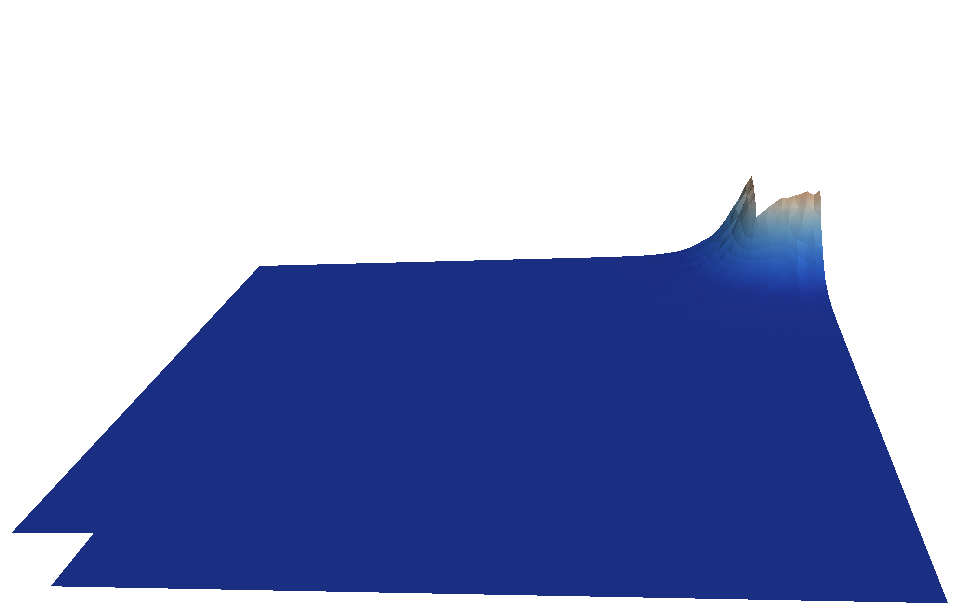
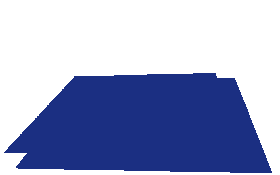
$\rho_{l}^{h}$ at $t=1200$ years	$p_{l}$ at $t=1200$ years	$S_{g}$ at $t=1200$ years
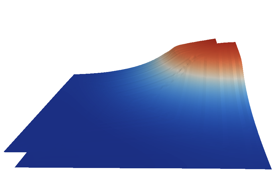
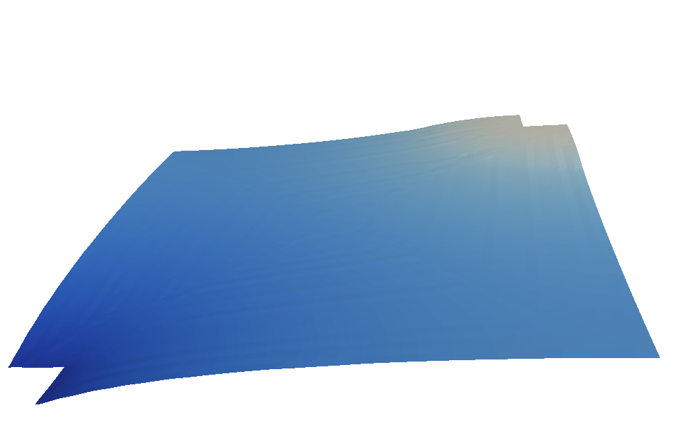
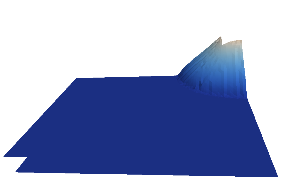
$\rho_{l}^{h}$ at $t=4\>10^{4}$ years	$p_{l}$ at $t=4\>10^{4}$ years	$S_{g}$ at $t=4\>10^{4}$ years
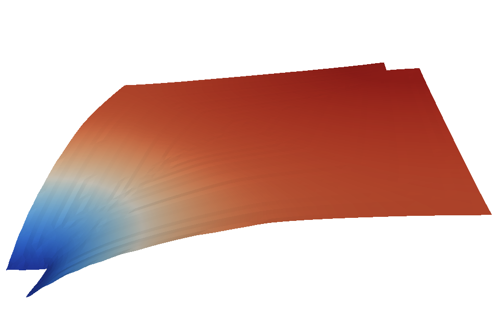
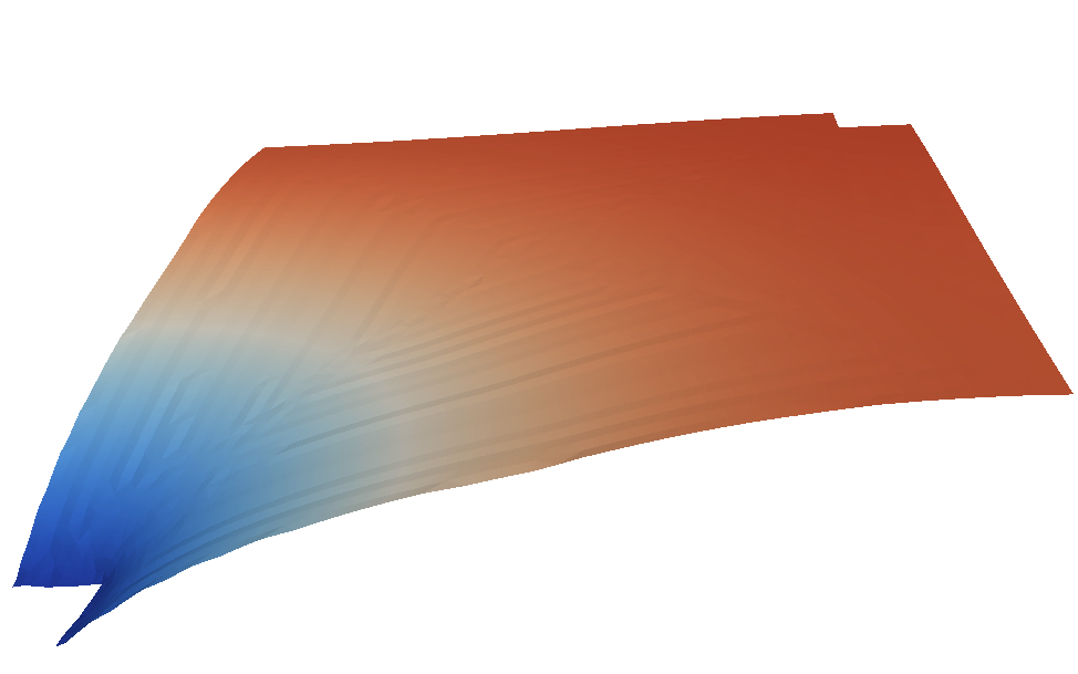
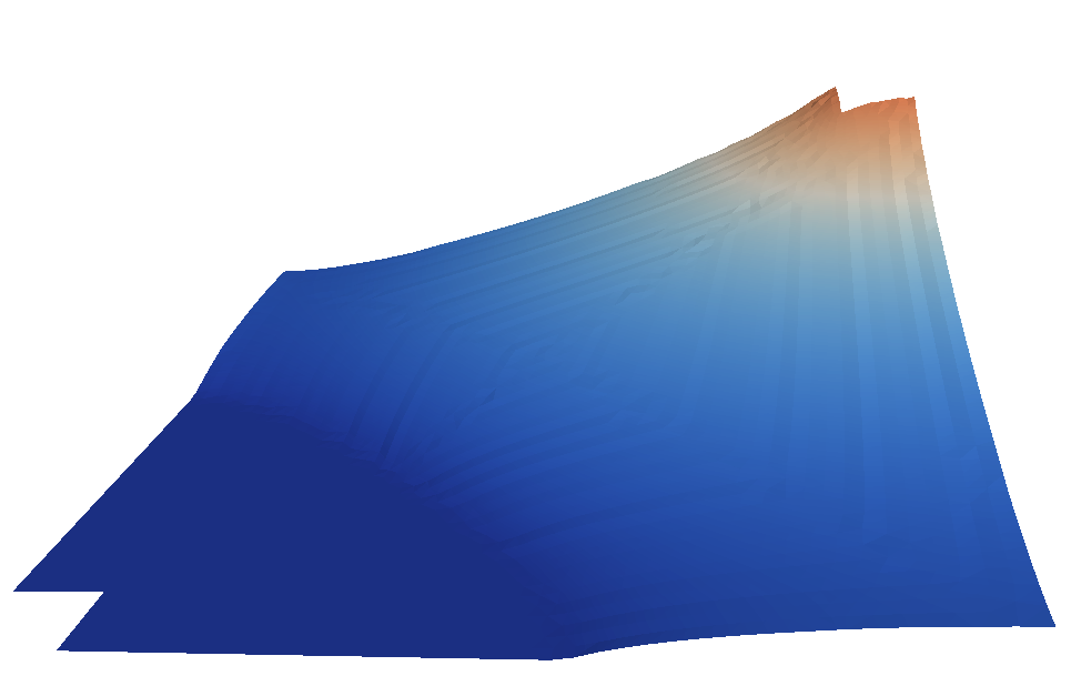
$\rho_{l}^{h}$ at $t=2\>10^{5}$ years	$p_{l}$ at $t=2\>10^{5}$ years	$S_{g}$ at $t=2\>10^{5}$ years
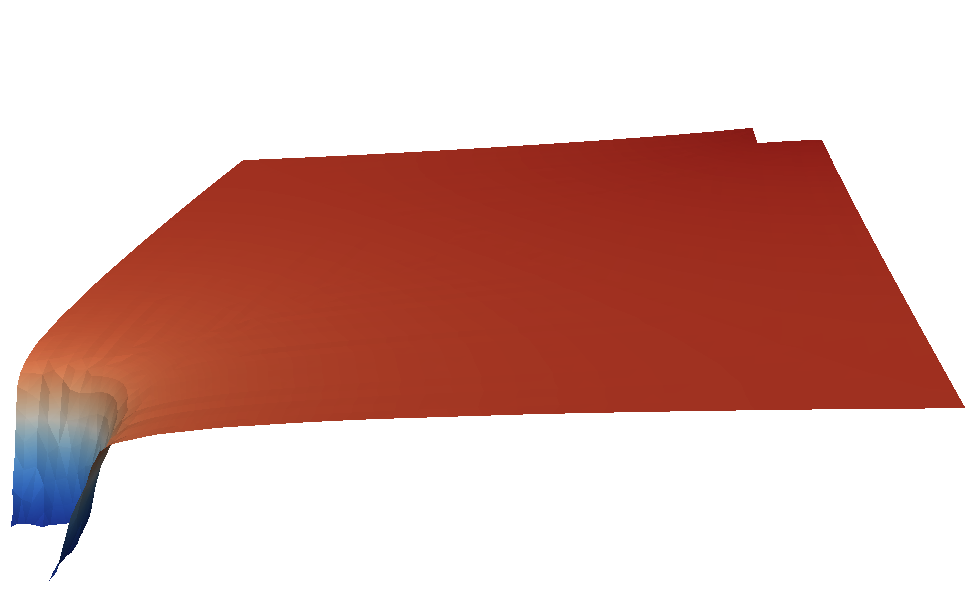
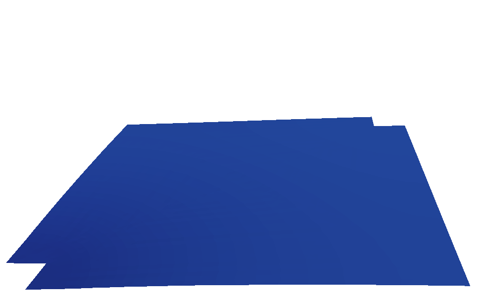
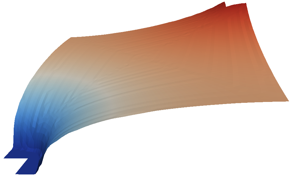
$\rho_{l}^{h}$ at $t=10^{6}$ years	$p_{l}$ at $t=10^{6}$ years	$S_{g}$ at $t=10^{6}$ years

Figure 5: Numerical Test case number 1: Evolution of $\rho_{l}^{h}$,the hydrogen concentration in the liquid phase; $p_{l}$ the liquid phase pressure; and $S_{g}$ the gas saturation ; at times $t=1200,4\>10^{4},2\>10^{5}$ and $10^{6}$ years (from the top to the bottom).

4.2 Numerical Test number 2

The geometry and the data of this numerical test are given in Figure 4 and Table 4. The porous medium is homogeneous and the initial conditions uniform; there is no need for defining two parts of the porous domain, $\Omega_{1}$ and $\Omega_{2}$; the parameter $L_{1}$ will be considered as null.

In this second test a constant flux of hydrogen is imposed on the input boundary $\Gamma_{in}$, while Dirichlet conditions $p_{l}=p_{l,out}$, $p_{g}=p_{g,out}$ are chosen, on $\Gamma_{out}$ , such that $\rho_{l}^{h}>C_{h}p_{l}$, in order to keep the gas phase ( according to the phase diagram in Figure 1) present on this part of the boundary. The initial conditions $p_{l}=p_{l,out}$ and $\rho_{l}^{h}=C_{h}p_{g,out}$ are uniform and imply the presence of the gas phase ( $S_{g}>0$) in the whole domain.

The main steps of the corresponding simulation are presented in Figures 6 and 7where are presented the liquid pressure $p_{l}$, the dissolved hydrogen molar density ( equal to $\rho_{l}^{h}/M^{h}$) and the gas saturation $S_{g}$ profiles at different times.

Boundary conditions	Porous medium			Others
Initial condition	Param.	Value		Param.	Value
$\phi^{w}\cdot\nu=0$ on $\Gamma_{imp}$	$k$	$5\;10^{-20}$	$m^{2}$	$L_{x}$	$200$	$m$
$\phi^{h}\cdot\nu=0$ on $\Gamma_{imp}$	$\Phi$	$0.15$	$(-)$	$L_{y}$	$20$	$m$
$\phi^{w}\cdot\nu=0$ on $\Gamma_{in}$	$P_{r}$	$2\;10^{6}$	$Pa$	$L_{1}$	$0$	$m$
$\phi^{h}\cdot\nu=\mathcal{Q}^{h}$ on $\Gamma_{in}$	$n$	$1.49$	$(-)$	$p_{l,out}$	$10^{6}$	$Pa$
$p_{l}=p_{l,out}$ on $\Gamma_{out}$	$S_{l,res}$	$0.4$	$(-)$	$p_{g,out}$	$1.1\;10^{6}$	$Pa$
$\rho_{l}^{h}=C_{h}p_{g,out}$ on $\Gamma_{out}$	$S_{g,res}$	$0$	$(-)$	$\mathcal{Q}^{h}$	$55.7$	$mg/m^{2}/year$
$p_{l}(t=0)=p_{l,out}$ in $\Omega$
$\rho_{l}^{h}(t=0)=C_{h}p_{g,out}$ in $\Omega$

Table 4: Numerical Test case number 2: Boundary and Initial Conditions; porous medium characteristics and domain geometry. $\phi^{w}$ and $\phi^{h}$ are denoting respectively the water and hydrogen flux.

At the beginning, up to $t<1400$ years, the two phases are present in the whole domain (see time $t=500$ years on Figure 6). The permanent injection of hydrogen increases both the two phase pressures and the gas saturation in the vicinity of $\Gamma_{in}$. The local gas saturation drop is due to the difference in mobilities between the two phases: the lower liquid mobility leads to a bigger liquid pressure increase, compared to the gas pressure increase; which is finally producing a capillary pressure drop (according to definition (3), see Figure 2), and creating a water saturated zone. At time $t=1400$ years, the gas phase starts to disappear in some region of the porous domain (see time $t=1500$ years, in Figure  7) .

Then, a saturated liquid region ($S_{g}=0$)will exist until time $t=17\;000$ years (see Figure  6); and during this period of time, the saturated region is pushed by the injected Hydrogen, from $\Gamma_{in}$ to $\Gamma_{out}$.

After the time $t=17\;000$ years, due to the Dirichlet conditions imposed on $\Gamma_{out}$, the liquid saturated region disappears and all together the phases pressure and the gas saturation are growing in the whole domain (see the time $t=20\;000$ years in Figure 7).

Finally the liquid pressure reaches its maximum at time $t=20\;000$ years and then decreases in the whole domain (see the Figure 7). This is caused, like in the numerical test case number 1, by the evolution of the system towards a stationary state which is characterized by a zero water component flow.

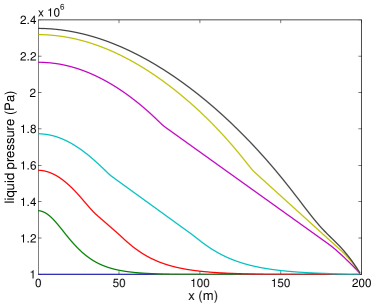
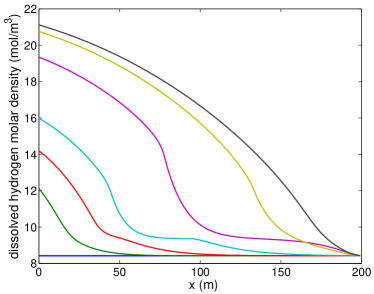
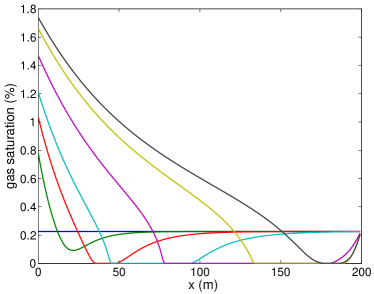
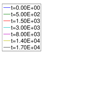
Figure 6: Test case number 2; $L_{x}=L_{2}=200$ m: Time evolution of $\rho_{l}^{h}$ (top right), the dissolved hydrogen molar density ($\rho_{l}^{h}/M^{h}$) (top left) and $S_{g}$ (bottom) profiles ; during the first time steps.

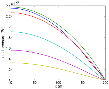
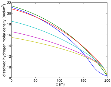
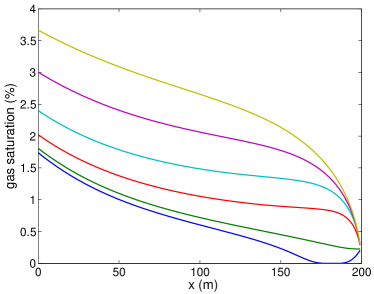
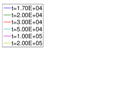
Figure 7: Test case number 2; $L_{x}=L_{2}=200$ m: Time evolution of the dissolved hydrogen molar density ($\rho_{l}^{h}/M^{h}$) (top right), $p_{l}$(top left) and $S_{g}$ (bottom) profiles ; during the six last time steps.

4.3 Numerical Test number 3

The geometry and the data of this numerical test are given in Figure 4 and Table 5 . Like in the Numerical Test number 2, a constant flux of hydrogen is imposed on the input boundary, $\Gamma_{in}$, while Dirichlet conditions $p_{l}=p_{l,out}$, $\rho_{l}^{h}=0$ are given on $\Gamma_{out}$, in order to have only the liquid phase on this part of the boundary. The initial conditions, $p_{l}=p_{l,out}$ and $\rho_{l}^{h}=0$, are uniform on all the domain, and correspond to a porous domain initially saturated with pure water. Contrary to the two first numerical tests, the porous domain is non homogeneous, there are two different porous subdomains $\Omega_{1}$ and $\Omega_{2}$; $L_{x}=200$ m, $L_{1}=20$ m and $L_{2}=180$ m.

Boundary conditions	Porous medium			Other
initial condition	Param.	Value on $\Omega_{1}$		Param.	Value
$\phi^{w}\cdot\nu=0$ on $\Gamma_{imp}$	$k$	$10^{-18}$	$m^{2}$	$L_{x}$	$200$	$m$
$\phi^{h}\cdot\nu=0$ on $\Gamma_{imp}$	$\Phi$	$0.3$	$(-)$	$L_{y}$	$20$	$m$
$\phi^{w}\cdot\nu=0$ on $\Gamma_{in}$	$P_{r}$	$2\;10^{6}$	$Pa$	$L_{1}$	$20$	$m$
$\phi^{h}\cdot\nu=\mathcal{Q}^{h}$ on $\Gamma_{in}$	$n$	$1.54$	$(-)$	$p_{l,out}$	$10^{6}$	$Pa$
$p_{l}=p_{l,out}$ on $\Gamma_{out}$	$S_{l,res}$	$0.01$	$(-)$	$\mathcal{Q}^{h}$	$5.57$	$mg/m^{2}/year$
$\rho_{l}^{h}=0$ on $\Gamma_{out}$	$S_{g,res}$	$0$	$(-)$
$p_{l}(t=0)=p_{l,out}$ on $\Omega$	Param.	Value on $\Omega_{2}$
$\rho_{l}^{h}(t=0)=0$ on $\Omega$	$k$	$5\;10^{-20}$	$m^{2}$
	$\Phi$	$0.15$	$(-)$
	$P_{r}$	$15\;10^{6}$	$Pa$
	$n$	$1.49$	$(-)$
	$S_{l,res}$	$0.4$	$(-)$
	$S_{g,res}$	$0$	$(-)$

Table 5: Numerical Test case number 3: Boundary and Initial Conditions; porous medium characteristics and domain geometry. $\phi^{w}$ and $\phi^{h}$ are denoting respectively the water and hydrogen flux.

Figure 8: Saturation discontinuity at the interface of two materials with different capillary pressure curves; test case number 3.

The simulation time of this test case is $T=10^{6}$ years;the discretization space mesh is 1 m; the time step is $10^{2}$ years at the beginning and grows up to $2\cdot 10^{4}$ years in the end of the simulation (see Table2).
Figures 9 and 10 represent the liquid pressure $p_{l}$, the dissolved hydrogen molar density ( equal to $\rho_{l}^{h}/M^{h}$) and the gas saturation $S_{g}$ profiles at different times.

The main difference from the previous simulations (which were in a homogeneous porous domain) is the gas saturation discontinuity, staying on the porous domain interface $x=20\;$m; and due to the height of this saturation jump , we had to use a logarithm scale for presenting the gas saturation $S_{g}$ profiles .

There are four main steps :

• From 0 to $3.8\cdot 10^{4}$ years both the gas saturation and the liquid pressure stay constant in the whole domain while the hydrogen injection on the left side $\Gamma_{in}$ of the domain increases the hydrogen density level .

• From $3.8\cdot 10^{4}$ to $5.4\cdot 10^{4}$ years both the liquid pressure and the hydrogen density are increasing in the whole domain. The gas start to expanding from the left side of the domain $\Gamma_{in}$. The saturation front is moved towards the porous media discontinuity, at $x=20\;m$, which is reached at $t=5.4\cdot 10^{4}$ years; see Figures 9.

• From $5.4\cdot 10^{4}$ years to $1.3\cdot 10^{5}$ years, see Figures 10, the saturation front has crossed the medium discontinuity at $x=20\;m$ and, from now, all the saturation profiles will have a discontinuity at $x=20\;m$.

• From $1.3\cdot 10^{5}$ years to $10^{6}$ years, see Figures 10, both the hydrogen density and the gas saturation keep growing while the liquid pressure decreases towards zero on the entire domain. The gas saturation front keeps moving to the right, pushed by the injected gas, up to $x\approx 150\;m$ at $10^{6}$ years.

Until the saturation front reaches the interface between the two porous media, for ($t=5.4\cdot 10^{4}$ years), appearance and evolution of both the gas phase and the unsaturated zone are identical to what was happening in the test case 1 (with a homogeneous porous domain) during the period of gas injection: the dissolved hydrogen is accumulating at the entrance until the liquid phase becomes saturated,at time ($t>3.8\>10^{4}$ years), letting the gas phase to appear.

When the saturation front crosses the interface between the two porous subdomains (at $x=20\;m$ and $t=5.4\cdot 10^{4}$ years), the gas saturation is strictly positive on both sides of this interface and the caplllary pressure curves being different on each side( see Table 5) forces the saturation to be discontinuous for preserving the capillary pressure continuity on the interface. The capillary pressure continuity at the interface imposes to $p_{c}^{(1)}$, the Capillary Pressure in $\Omega_{1}$, and to $p_{c}^{(2)}$, the Capillary Pressure in $\Omega_{2}$, to be equal on this interface. $p_{c}^{(1)}=p_{c}^{(2)}$ is satisfied only if there are two different saturations,on each interface side $S_{g}^{(1)}$, and $S_{g}^{(2)}$: $p_{c}^{(1)}(S_{g}^{(1)})=p_{c}^{(2)}(S_{g}^{(2)})$ ; see Figure 8.

In the same way as in the numerical test case number 1, the system tends to a stationary state

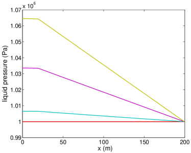
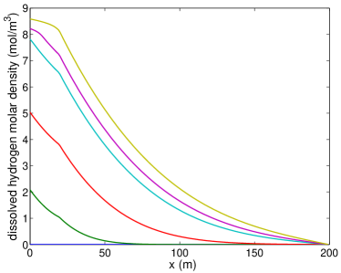
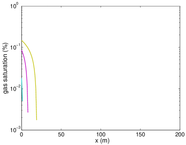
Figure 9: Test case number 3; $L_{x}=200$ m, $L_{1}=20$m: Time evolution of the dissolved hydrogen molar density ($\rho_{l}^{h}/M^{h}$) (top right), $p_{l}$ (top left) and $S_{g}$ (bottom) profiles ; during the first time steps. All the $S_{g}$ curves go to zero( although this cannot be seen using a logarithmic scale) .

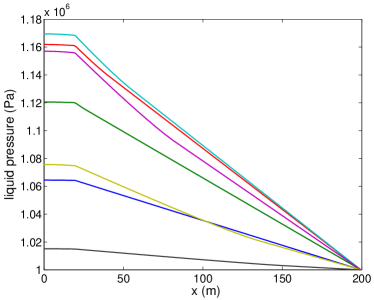
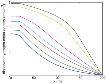
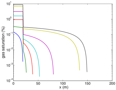
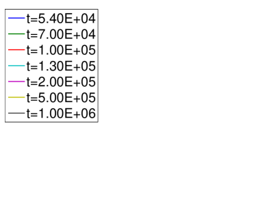
Figure 10: Test case number 3; $L_{x}=200$ m, $L_{1}=20$m: Time evolution of the dissolved hydrogen molar density ($\rho_{l}^{h}/M^{h}$)(top right), $p_{l}$ (top left) and $S_{g}$ (bottom) profiles ; during the last seven time steps. All the $S_{g}$ curves go to zero( although this cannot be seen using a logarithmic scale) .

4.4 Numerical Test number 4

This last numerical test is different from all the precedent ones; it intends to be a simplified representation of what happens when an unsaturated porous block is placed within a water saturated porous structure. The challenge is then: how the mechanical balance will be restored in a homogeneous porous domain , which was initially out of equilibrium, i.e. with a jump in the initial phase pressures?

The initial liquid pressure is the same in the entire porous domain; $\Omega$ ,$p_{l,1}=p_{l,2}$ , and in the subdomain $\Omega_{1}$ the initial condition, ($p_{l,1}=p_{g,1}$ in Table 6, corresponds to a liquid fully saturated state with a hydrogen concentration reaching the gas appearance concentration threshold ($p_{g}=p_{l}$ and $\rho_{l}^{h}=C_{h}p_{g}$, see Figure 1). In the subdomain $\Omega_{2}$ the initial condition($p_{l,2}\neq p_{g,2}$and $p_{g,2}\neq p_{g,1}$ )corresponds to a non saturated state (see Table 6).
The porous block initial state is said out of equilibrium, because:
if this initial state was in equilibrium , in the two subdomains $\Omega_{1}\;$ and $\Omega_{2}$, the local mechanical balance would have made the pressures, of both the liquid and the gas phase, continuous in the entire domain $\Omega\;$.

For simplicity, we assume the porous medium domain $\Omega$ is homogeneous and all the porous medium characteristics are the same in the two subdomains $\Omega_{1}$ and $\Omega_{2}$, and corresponding to concrete.

The system is then expected to evolve from this initial out of equilibrium state towards a stationary state.

We should notice that, in order to see appearing the final stationary state, in a reasonable period of time, we have shortened the domain $\Omega$ ( $L_{x}=1$m), taken the porous media characteristics , and set the final time of this simulation $T_{fin}$ at $T_{fin}=10^{6}\;s\approx 11.6\;$) days. The complete set of data of this test case is given in Table 6.

Boundary conditions	Porous medium			Other
initial condition	Param.	Value		Param.	Value
$\phi^{w}\cdot\nu=0$ on $\partial\Omega$	$k$	$10^{-18}$	$m^{2}$	$L_{x}$	$1$	$m$
$\phi^{h}\cdot\nu=0$ on $\partial\Omega$	$\Phi$	$0.3$	$(-)$	$L_{y}$	$0.1$	$m$
$p_{l}(t=0)=p_{l,1}$ on $\Omega_{1}$	$P_{r}$	$2\;10^{6}$	$Pa$	$L_{1}$	$0.5$	$m$
$\rho_{l}^{h}(t=0)=C_{h}p_{g,1}$ on $\Omega_{1}$	$n$	$1.54$	$(-)$	$p_{l,1}$	$10^{6}$	$Pa$
$p_{l}(t=0)=p_{l,2}$ on $\Omega_{2}$	$S_{l,res}$	$0.01$	$(-)$	$p_{g,1}$	$10^{6}$	$Pa$
$\rho_{l}^{h}(t=0)=C_{h}p_{g,2}$ on $\Omega_{2}$	$S_{g,res}$	$0$	$(-)$	$p_{l,2}$	$10^{6}$	$Pa$
				$p_{g,2}$	$2.5\;10^{6}$	$Pa$

Table 6: Data of the numerical test number 4 : boundary and initial conditions;domain geometry. The porous medium domain $\Omega$ is homogeneous, all the porous medium parameters are the same in the two subdomains $\Omega_{1}$ and $\Omega_{2}$; $\phi^{w}$ and $\phi^{h}$ are denoting respectively the water and hydrogen flux .

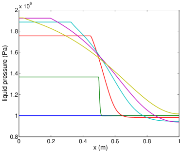
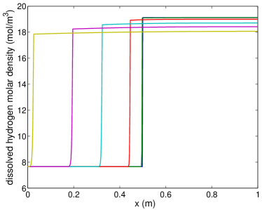
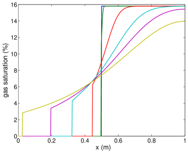
Figure 11: Numerical test case number 4, $L_{x}=1$ m, $L_{1}=0.5$ m: Time evolution of the dissolved hydrogen molar density ($\rho_{l}^{h}/M^{h}$) (top right), $p_{l}$ (top left) and $S_{g}$ (bottom) profiles; during the six first time steps.

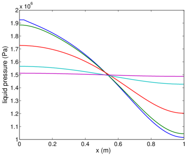
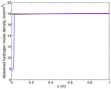
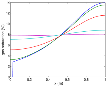
Figure 12: Numerical test case number 4, $L_{x}=1$ m, $L_{1}=0.5$ m: Time evolution of the the dissolved hydrogen molar density ($\rho_{l}^{h}/M^{h}$) (top right), $p_{l}$ (top left) and $S_{g}$ (bottom) profiles; during the five last time steps.

The space discretization step was taken constant equal to $2\cdot 10^{-3}$ m and the time step was variable, going from $0.33~{}s$ in the beginning of the simulation to $16.7\cdot 10^{3}\;s$ at the end of the simulation (see Table  2). Figures 11 and 12 represent the liquid pressure $p_{l}$, the dissolved hydrogen molar density ( equal to $\rho_{l}^{h}/M^{h}$) and the gas saturation $S_{g}$ profiles at different times.

There are essentially two steps:

• For $0<t<1.92\cdot 10^{5}\;s$ (see Figure 11), the initial gas saturation jump moves from $x=0.5~{}m$, at $t=0$ and reaches $\Gamma_{in}$, the left domain boundary, at $t=1.92\cdot 10^{5}~{}s$. During this movement, the saturation jump height (initially $\approx 0.16\;$) decreases, until approximately $0.03$, when it reaches the left boundary $\Gamma_{in}$. In front of this discontinuity there is a liquid saturated zone, $S_{g}=0$, and in this zone both the liquid pressure and the hydrogen density are spatially uniform (see Figure 11, top ). But, while the hydrogen density remains constant and equal to its initial value, the liquid pressure becomes immediately continuous and starts growing quickly (for instance, $p_{l}(t=10^{3}\;s)\approx 1.6\cdot 10^{6}\;$Pa), and then more slowly until $t=1.3\cdot 10^{5}\;s$, when it starts to slightly decrease.

  In Figure 11, located on the gas saturation discontinuity, there are both a high contrast in the dissolved hydrogen concentration (this concentration stays however continuous, but with a strong gradient, as seen in the top right of Figure 11), and a discontinuity in the liquid pressure gradient (see the top left of Figure 11).

• For $1.92\cdot 10^{5}\;s<t<10^{6}\;s=T_{fin}$ (see Figure  12), all the entire domain is now unsaturated ($S_{g}>$0). The liquid pressure, the hydrogen density and the gas saturation profiles are all strictly monotonous and continuous, going towards a spatially uniform distribution, corresponding to the stationary state(see Figure 12).

As expected, the system initially out of equilibrium (discontinuity of the gas pressure), becomes immediately again in equilibrium (the gas pressure is continuous)and evolves towards a uniform stationary state (due to the no mass inflow and outflow boundary conditions). Although the liquid pressure and the dissolved hydrogen density are immediately again continuous for $t>0\;$, the hydrogen density still have a locally very strong gradient until $t=1.92\cdot 10^{5}\;s$.

At first, and at the very begining($\approx~{}10^{2}\;s$), see top left of Figure 11, only the liquid pressure evolves in the liquid saturated zone. Due to a gas pressure in the unsaturated zone higher than in the liquid saturated zone ($S_{g}=0$; $p_{g}=2.5MPa>p_{l}=1MPa$, for the initial state in Table6), and due to the no flow condition imposed on $\Gamma_{in}$, the liquid in the saturated zone is compressed by the gas from the unsaturated zone. Then, a liquid gradient pressure appears around the saturation front and makes the liquid to flow from the liquid saturated zone towards the unsaturated one, and then the gas saturation front to move in the opposite direction.

The very strong hydrogen density gradient (until $t=1.92\cdot 10^{5}\;s$), located on the saturation front, is due to the competition between the diffusion and the convective flux of the dissolved hydrogen around the saturation front: the water flow convecting the dissolved hydrogen, from left to right, cancels the smoothing effect of the gas diffusion propagation in the opposite direction. On the one hand the diffusion is supposed to reduce the hydrogen concentration contrast, by creating a flux going from strong concentrations (in the unsaturated zone) towards the low concentrations (in the liquid saturated zone), and on the other hand the flow of the liquid phase goes in the opposite direction (left to right, from $S_{g}=0$ to $S_{g}>0$). Once the disequilibrium has disappeared, the system tends to reach a uniform stationary state determined by the mass conservation of each component present in the initial state (the system is isolated, with no flow on any of the boundaries).

5 Concluding remarks

From balance equations, constitutive relations and equations of state, assuming thermodynamical equilibrium, we have derived a model for describing underground gas migration in water saturated or unsaturated porous media, including diffusion of components in phases and capillary effects. In the second part, we have presented a group of numerical test cases synthesizing the main challenges concerning gas migration in a deep geological repository. These numerical simulations, are based on simplified but typical situations in underground nuclear waste management; they show evidence of the model ability to describe the gas (hydrogen) migration, and to treat the difficult problem of correctly following the saturated and unsaturated regions created by the gas generation.

Acknowledgements 1

This work was partially supported by the GNR MoMaS
(PACEN/CNRS, ANDRA, BRGM, CEA, EDF, IRSN). Most of the work on this paper was done when Mladen Jurak was visiting, at Université Lyon 1, the CNRS-UMR 5208 ICJ.

References

• [1] Abadpour A., Panfilov M.: Method of Negative Saturations for two-phase Compositional Flow with Oversaturated Zones, Transport in Porous Media 79; 197-214 (2009).
• [2] Bourgeat, A., Jurak, M. and Smaï, F.: Two partially miscible flow and transport modeling in porous media; application to gas migration in a nuclear waste repository, Computational Geosciences 13(1), 29-42 (2009).
• [3] CEA, Cast3m, http://www-cast3m.cea.fr/cast3m/index.jsp
• [4] Jaffré, J. and Sboui, A.: Henry’ Law and Gas Phase Disappearance, ”INRIA report 6891” (2009), to appear in Transport in Porous Media.