Credit Risk, Market Sentiment and Randomly-Timed Default

Abstract

We propose a model for the credit markets in which the random default times of bonds are assumed to be given as functions of one or more independent “market factors”. Market participants are assumed to have partial information about each of the market factors, represented by the values of a set of market factor information processes. The market filtration is taken to be generated jointly by the various information processes and by the default indicator processes of the various bonds. The value of a discount bond is obtained by taking the discounted expectation of the value of the default indicator function at the maturity of the bond, conditional on the information provided by the market filtration. Explicit expressions are derived for the bond price processes and the associated default hazard rates. The latter are not given a priori as part of the model but rather are deduced and shown to be functions of the values of the information processes. Thus the “perceived” hazard rates, based on the available information, determine bond prices, and as perceptions change so do the prices. In conclusion, explicit expressions are derived for options on discount bonds, the values of which also fluctuate in line with the vicissitudes of market sentiment.

I Credit-risk modelling

In this paper we consider a simple model for defaultable securities and, more generally, for a class of financial instruments for which the cash flows depend on the default times of a set of defaultable securities. For example, if $\tau$ is the time of default of a firm that has issued a simple credit-risky zero-coupon bond that matures at time $T$, then the bond delivers a single cash-flow $H_{T}$ at $T$, given by

$$H_{T}=N\,{\mathds{1}}\{\tau>T\},$$ (1)

where $N$ is the principal, and ${\mathds{1}}\{\tau>T\}=1$ if $\tau>T$ and ${\mathds{1}}\{\tau>T\}=0$ if $\tau\leq T$. By a “simple” credit-risky zero-coupon bond we mean the case of an idealised bond where there is no recovery of the principal if the firm defaults. If a fixed fraction $R$ of the principal is paid at time $T$ in the event of default then we have

$$H_{T}=N{\mathds{1}}\{\tau>T\}+RN{\mathds{1}}\{\tau\leq T\}.$$ (2)

More realistic models can be developed by introducing random factors that determine the amount and timing of recovery levels. See, e.g., Brody, Hughston & Macrina (2007, 2010), and Macrina & Parbhoo (2010).

As another example, let $\tau_{1},\tau_{2}\ldots,\tau_{n}$ denote the default times of a set of $n$ discount bonds, each with maturity after $T$. Write $\bar{\tau}_{1},\bar{\tau}_{2},\ldots,\bar{\tau}_{n}$ for the “order statistics” of the default times. Hence $\bar{\tau}_{1}$ is the time of the first default (among $\tau_{1},\tau_{2},\ldots,\tau_{n})$, $\bar{\tau}_{2}$ is the time of the second default, and so on. Then a structured product that pays

$$H_{T}=K\,{\mathds{1}}\{\bar{\tau}_{k}\leq T\}$$ (3)

is a kind of insurance policy that pays $K$ at time $T$ if there have been $k$ or more defaults by time $T$.

One of the outstanding problems associated with credit-risk modelling is the following. What counts in the valuation of credit-risky products is not necessarily the “actual” or “objective” probability of default (even if this can be meaningfully determined), but rather the “perceived” probability of default. This can change over time, depending on shifts in market sentiment and the flow of relevant market information. How do we go about modelling the dynamics of such products?

II Modelling the market filtration

We introduce a probability space with a measure ${\mathbb{Q}}$ which, for simplicity, we take to be the risk-neutral measure. Thus, the price process of any non-dividend-paying asset, when the price is expressed in units of a standard money-market account, is a $\mathbb{Q}$-martingale. We do not assume that the market is necessarily complete; rather, we merely assume that there is an established pricing kernel. We assume, again for simplicity, that the default-free interest-rate term structure is deterministic. Time $0$ denotes the present, and we write $P_{tT}$ for the price at $t$ of a default-free discount bond that matures at $T$. To ensure absence of arbitrage, we require that $P_{tT}=P_{0T}/P_{0t}$, where $\{P_{0t}\}_{0\leq t<\infty}$ is the initial term structure. No attempt will be made in the present investigation to examine the case of stochastic interest rates: to keep credit-related issues in the foreground, we suppress considerations relating to the default-free interest rate term structure. See Rutkowski & Yu (2007), Hughston & Macrina (2009), Brody & Friedman (2009), and Macrina & Parbhoo (2010) for discussions of the stochastic interest rate case in an information-based setting.

The probability space comes equipped with a filtration $\{{\mathcal{G}}_{t}\}$ which we take to be the market filtration. Our first objective is to define $\{{\mathcal{G}}_{t}\}$ in such a way that market sentiments concerning the default times can be modelled explicitly. We let $\tau_{1}$, $\tau_{2}$, …,$\tau_{n}$ be a collection of non-negative random times such that ${\mathbb{Q}}(\tau_{\alpha}=0)=0$ and ${\mathbb{Q}}(\tau_{\alpha}>t)>0$ for $t>0$ and $\alpha=1,2,\ldots,n$. We set

$$\tau_{\alpha}=f_{\alpha}(X_{1},X_{2},\ldots,X_{N}),\qquad(\alpha=1,2,\ldots,n).$$ (4)

Here $X_{1},X_{2},\ldots,X_{N}$ are $N$ independent, continuous, real-valued market factors that determine the default times, and $f_{\alpha}$ for each $\alpha$ is a smooth function of $N$ variables that determines the dependence of $\tau_{\alpha}$ on the market factors. We note that if two default times share an $X$-factor in common, then they will in general be correlated. With each $\tau_{\alpha}$ we associate a “survival” indicator process ${\mathds{1}}\{\tau_{\alpha}>t\}$, $t\geq 0$, which takes the value unity until default occurs, at which time it drops to zero. Additionally, we introduce a set of $N$ information processes $\{\xi^{k}_{t}\}_{t\geq 0}$ in association with the market factors, which in the present investigation we take to be of the form

$$\xi^{k}_{t}=\sigma_{k}tX_{k}+B^{k}_{t}.$$ (5)

Here, for each $k$, $\sigma_{k}$ is a parameter (“information flow rate”) and $\{B^{k}_{t}\}_{t\geq 0}$ is a Brownian motion (“market noise”). We assume that the $X$-factors and the market noise processes are all independent of one another.

We take the market filtration $\{{\mathcal{G}}_{t}\}_{t\geq 0}$ to be generated jointly by the information processes and the survival indicator processes. Therefore, we have:

$${\mathcal{G}}_{t}={\boldsymbol{\sigma}}\left[\{\xi_{s}^{k}\}_{0\leq s\leq t}^{k=1,\ldots,N},{\mathds{1}}\{\tau^{\alpha}>s\}^{\alpha=1,\ldots,n}_{0\leq s\leq t}\right].$$ (6)

It follows that at $t$ the market knows the information generated up to $t$ and the history of the indicator processes up to time $t$. For the purpose of calculations it is useful also to introduce the filtration $\{{\mathcal{F}}_{t}\}_{t\geq 0}$ generated by the information processes:

$${\mathcal{F}}_{t}={\boldsymbol{\sigma}}\left[\{\xi_{s}^{k}\}^{k=1,\ldots,N}_{0\leq s\leq t}\right].$$ (7)

Then clearly ${\mathcal{F}}_{t}\subset{\mathcal{G}}_{t}$. We do not require as such the notion of a “background” filtration for our theory. Indeed, we can think of the $\xi$’s and the ${\mathds{1}}$’s as providing two related but different types of information about the $X$’s.

III Credit-risky discount bond

As an example we study in more detail the case $n=1$, $N=1$. We have a single random market factor $X$ and an associated default time $\tau=f(X)$. We assume that $X$ is continuous and that $f(X)$ is monotonic. The market filtration $\{{\mathcal{G}}_{t}\}$ is generated jointly by an information process of the form

$$\xi_{t}=\sigma tX+B_{t},\qquad t\geq 0,$$ (8)

and the indicator process ${\mathds{1}}\{\tau>t\}$, $t\geq 0$. The Brownian motion $\{B_{t}\}_{t>0}$ is taken to be independent of $X$. The value of a defaultable $T$-maturity discount bond, when there is no recovery on default, is then given by

$$B_{tT}=P_{tT}\,{\mathbb{E}}\left[{\mathds{1}}\{\tau>T\}\,|\,{\mathcal{G}}_{t}\right]$$ (9)

for $0\leq t\leq T$. We shall write out an explicit expression for $B_{tT}$. First, we use the identity (see, e.g., Bielecki, Jeanblanc & Rutkowski 2009):

$${\mathbb{E}}\left[{\mathds{1}}\{\tau>T\}\,|\,{\mathcal{G}}_{t}\right]={\mathds{1}}\{\tau>t\}\frac{{\mathbb{E}}\left[{\mathds{1}}\{\tau>T\}|{\mathcal{F}}_{t}\right]}{{\mathbb{E}}\left[{\mathds{1}}\{\tau>t\}|{\mathcal{F}}_{t}\right]},$$ (10)

where ${\mathcal{F}}_{t}$ is as defined in (7). It follows that

$$B_{tT}=P_{tT}{\mathds{1}}\{\tau>t\}\frac{{\mathbb{E}}\left[{\mathds{1}}\{\tau>T\}|{\mathcal{F}}_{t}\right]}{{\mathbb{E}}\left[{\mathds{1}}\{\tau>t\}|{\mathcal{F}}_{t}\right]}.$$ (11)

We note that the information process $\{\xi_{t}\}$ has the Markov property with respect to its own filtration. To see this, it suffices to check that

$${\mathbb{Q}}\left(\xi_{t}\leq x|\xi_{s},\xi_{s_{1}},\xi_{s_{2}},\ldots,\xi_{s_{k}}\right)={\mathbb{Q}}\left(\xi_{t}\leq x|\xi_{s}\right)$$ (12)

for any collection of times $t\geq s\geq s_{1}\geq s_{2}\geq\cdots\geq s_{k}>0$. We observe that for $s>s_{1}>s_{2}>s_{3}>0$, the random variables $\{B_{s}/s-B_{s_{1}}/s_{1}\}$ and $\{B_{s_{2}}/s_{2}-B_{s_{3}}/s_{3}\}$ are independent. This follows directly from a calculation of their covariance. Hence from the relation

$$\frac{\xi_{s}}{s}-\frac{\xi_{s_{1}}}{s_{1}}=\frac{B_{s}}{s}-\frac{B_{s_{1}}}{s_{1}}$$ (13)

we conclude that

$${\mathbb{Q}}\left(\xi_{t}\leq x|\xi_{s},\xi_{s_{1}},\ldots,\xi_{s_{k}}\right) = {\mathbb{Q}}\left(\xi_{t}\leq x|\xi_{s},\frac{\xi_{s}}{s}-\frac{\xi_{s_{1}}}{s_{1}},\frac{\xi_{s_{1}}}{s_{1}}-\frac{\xi_{s_{2}}}{s_{2}},\ldots,\frac{\xi_{s_{k-1}}}{s_{k-1}}-\frac{\xi_{s_{k}}}{s_{k}}\right)$$ (14)

$$={\mathbb{Q}}\left(\xi_{t}\leq x|\xi_{s},\frac{B_{s}}{s}-\frac{B_{s_{1}}}{s_{1}},\frac{B_{s_{1}}}{s_{1}}-\frac{B_{s_{2}}}{s_{2}},\ldots,\frac{B_{s_{k-1}}}{s_{k-1}}-\frac{B_{s_{k}}}{s_{k}}\right).$$

However, since $\xi_{t}$ and $\xi_{s}$ are independent of $B_{s}/s-B_{s_{1}}/s_{1}$, $B_{s_{1}}/s_{1}-B_{s_{2}}/s_{2}$, $\ldots$, $B_{s_{k-1}}/s_{k-1}-B_{s_{k}}/s_{k}$, the result (12) follows.

As a consequence of the Markovian property of $\{\xi_{t}\}$ and the fact that $X$ is ${\mathcal{F}}_{\infty}$-measurable, we therefore obtain

$$B_{tT}=P_{tT}{\mathds{1}}\{\tau>t\}\,\frac{{\mathbb{E}}\left[{\mathds{1}}\{\tau>T\}\,|\,\xi_{t}\right]}{{\mathbb{E}}\left[{\mathds{1}}\{\tau>t\}\,|\,\xi_{t}\right]}$$ (15)

for the defaultable bond price. Thus we can write

$$B_{tT}=P_{tT}\,{\mathds{1}}\{\tau>t\}\,\frac{\int^{\infty}_{-\infty}{\mathds{1}}\{f(x)>T\}\rho_{t}(x)\mbox{$\rm d$}x}{\int^{\infty}_{-\infty}{\mathds{1}}\{f(x)>t\}\rho_{t}(x)\mbox{$\rm d$}x}.$$ (16)

Here

$$\rho_{t}(x)={\mathbb{E}}\left[\delta(X-x)\,|\,\xi_{t}\right]$$ (17)

is the conditional density for $X$ given $\xi_{t}$, and a calculation using the Bayes law shows that:

$$\rho_{t}(x)=\frac{\rho_{0}(x)\exp\left[\sigma x\xi_{t}-\frac{1}{2}\sigma^{2}x^{2}t\right]}{\int_{-\infty}^{\infty}\rho_{0}(x)\exp\left[\sigma x\xi_{t}-\frac{1}{2}\sigma^{2}x^{2}t\right]\mbox{$\rm d$}x},$$ (18)

where $\rho_{0}(x)$ is the a priori density of $X$. Thus for the bond price we obtain:

$$B_{tT}=P_{tT}{\mathds{1}}\{\tau>t\}\,\frac{\int^{\infty}_{-\infty}\rho_{0}(x){\mathds{1}}\{f(x)>T\}\exp\left[\sigma x\xi_{t}-\frac{1}{2}\sigma^{2}x^{2}t\right]\mbox{$\rm d$}x}{\int^{\infty}_{-\infty}\rho_{0}(x){\mathds{1}}\{f(x)>t\}\exp\left[\sigma x\xi_{t}-\frac{1}{2}\sigma^{2}x^{2}t\right]\mbox{$\rm d$}x}.$$ (19)

It should be apparent that the value of the bond fluctuates as $\xi_{t}$ changes. This reflects the effects of changes in market sentiment concerning the possibility of default. Indeed, if we regard $\tau$ as the default time of an obligor that has issued a number of different bonds (coupon bonds can be regarded as bundles of zero-coupon bonds), then similar formulae will apply for each of the various bond issues.

When the default times of two or more distinct obligors depend on a common market factor, the resulting bond price dynamics are correlated and so are the default times. The modelling framework presented here therefore provides a basis for a number of new constructions in credit-risk management, including explicit expressions for the volatilities and correlations of credit-risky bonds.

Our methodology is to consider models for which each independent $X$-factor has its own information process. Certainly, we can also consider the situation where there may be two or more distinct information processes available concerning the same $X$-factor. This situation is relevant to models with asymmetric information, where some traders may have access to “more” information about a given market factor than other traders; see Brody, Davis, Friedman & Hughston (2008), Brody, Brody, Meister & Parry (2010), and Brody, Hughston & Macrina (2010).

In principle, a variety of different types of information processes can be considered. We have in (5) used for simplicity what is perhaps the most elementary type of information process, a Brownian motion with a random drift. The linearity of the drift term in the time variable ensures on the one hand that the information process has the Markov property, and on the other hand, since the Brownian term grows in magnitude on average like the square-root of time, that the drift term eventually comes to dominate the noise term, thus allowing for the release of information concerning the likely time of default. Information processes based variously on the Brownian bridge (Brody, Hughston & Macrina 2007, 2008a), the gamma bridge (Brody, Hughston & Macrina 2008b), and the Lévy bridge (Hoyle, Hughston & Macrina 2009, 2010) have been applied to problems in finance and insurance.

Our work can be viewed in the context of the growing body of literature on the role of information in finance and its application to credit risk modelling in particular. No attempt will be made here at a systematic survey of material in this line. We refer the reader, for example, to Föllmer, Wu, & Yor (1999), Kusuoka (1999), Duffie & Lando (2001), Jarrow & Protter (2004), Çetin, Jarrow, Protter & Yildirim (2004), Giesecke (2006), Geman, Madan, & Yor (2007), Coculescu, Geman & Jeanblanc (2008), Frey & Schmidt (2009), Bielecki, Jeanblanc & Rutkowski (2009), and works cited therein.

IV Discount bond dynamics

Further insight into the nature of the model can be gained by working out the dynamics of the bond price. An application of Ito calculus gives the following dynamics over the time interval from $0$ to $T$:

$$\mbox{$\rm d$}B_{tT}=(r_{t}+h_{t})B_{tT}\mbox{$\rm d$}t+\sigma\Sigma_{tT}\,B_{tT}\mbox{$\rm d$}W_{t}+B_{t^{-}T}\mbox{$\rm d$}{\mathds{1}}\{\tau>t\}.$$ (20)

Here

$$r_{t}=-\partial_{t}\ln(P_{0t})$$ (21)

is the deterministic short rate of interest, and

$$h_{t}=\frac{{\mathbb{E}}\left[\delta(f(X)-t)\,|\,{\mathcal{F}}_{t}\right]}{{\mathbb{E}}\left[{\mathds{1}}\{f(X)>t\}\,|\,{\mathcal{F}}_{t}\right]}$$ (22)

is the so-called hazard rate. It should be evident that if $\tau\leq T$ then when the default time is reached the bond price drops to zero. The defaultable discount bond volatility $\Sigma_{tT}$ is given by

$$\Sigma_{tT}=\frac{{\mathbb{E}}\left[{\mathds{1}}\{f(X)>T\}X\,|\,{\mathcal{F}}_{t}\right]}{{\mathbb{E}}\left[{\mathds{1}}\{f(X)>T\}\,|\,{\mathcal{F}}_{t}\right]}-\frac{{\mathbb{E}}\left[{\mathds{1}}\{f(X)>t\}X\,|\,{\mathcal{F}}_{t}\right]}{{\mathbb{E}}\left[{\mathds{1}}\{f(X)>t\}\,|\,{\mathcal{F}}_{t}\right]}.$$ (23)

The process $\{W_{t}\}$ appearing in the dynamics of $\{B_{tT}\}$ is defined by the relation:

$$W_{t}=\int^{t}_{0}\!\!{\mathds{1}}\{f(X)>s\}\left(\mbox{$\rm d$}\xi_{s}-\sigma{\mathbb{E}}\left[X|{\mathcal{G}}_{s}\right]\mbox{$\rm d$}s\right).$$ (24)

To deduce the formulae above we define a one-parameter family of $\{\mathcal{F}_{t}\}$-adapted processes $\{F_{tu}\}$ by setting

$$F_{tu}=\int^{\infty}_{-\infty}\rho_{0}(x){\mathds{1}}\{f(x)>u\}\exp\left[\sigma x\xi_{t}-\mbox{$\textstyle\frac{1}{2}$}\sigma^{2}x^{2}t\right]\mbox{$\rm d$}x.$$ (25)

Then the bond price can be written in the form

$$B_{tT}=P_{tT}{\mathds{1}}\{\tau>t\}\frac{F_{tT}}{F_{tt}}.$$ (26)

An application of Ito’s lemma gives

$$\frac{\mbox{$\rm d$}F_{tT}}{F_{tT}}=\sigma\frac{{\mathbb{E}}\left[{\mathds{1}}\{f(X)>T\}X\,|\,{\mathcal{F}}_{t}\right]}{{\mathbb{E}}\left[{\mathds{1}}\{f(X)>T\}\,|\,{\mathcal{F}}_{t}\right]}\,\mbox{$\rm d$}\xi_{t}$$ (27)

and

$$\frac{\mbox{$\rm d$}F_{tt}}{F_{tt}}=-\frac{{\mathbb{E}}\left[\delta(f(X)-t)\,|\,{\mathcal{F}}_{t}\right]}{{\mathbb{E}}\left[{\mathds{1}}\{f(X)>t\}\,|\,{\mathcal{F}}_{t}\right]}\,\mbox{$\rm d$}t+\sigma\frac{{\mathbb{E}}\left[{\mathds{1}}\{f(X)>T\}X\,|\,{\mathcal{F}}_{t}\right]}{{\mathbb{E}}\left[{\mathds{1}}\{f(X)>T\}\,|\,{\mathcal{F}}_{t}\right]}\,\mbox{$\rm d$}\xi_{t}.$$ (28)

The desired results then follow at once by use of the relation

$$\mbox{$\rm d$}\left(\frac{F_{tT}}{F_{tt}}\right)=\frac{F_{tT}}{F_{tt}}\left[\frac{\mbox{$\rm d$}F_{tT}}{F_{tT}}-\frac{\mbox{$\rm d$}F_{tt}}{F_{tt}}+\left(\frac{\mbox{$\rm d$}F_{tt}}{F_{tt}}\right)^{2}-\frac{\mbox{$\rm d$}F_{tT}}{F_{tT}}\frac{\mbox{$\rm d$}F_{tt}}{F_{tt}}\right].$$ (29)

The process $\{W_{t}\}_{0\leq t<\tau}$ defined by (24) is a $\{{\mathcal{G}}_{t}\}$-Brownian motion. This can be seen by use of Lévy’s characterisation. Specifically, we have $\mbox{$\rm d$}W_{t}^{2}=\mbox{$\rm d$}t^{2}$ and ${\mathbb{E}}[W_{u}\,|\,\mathcal{G}_{t}]=W_{t}$. To see that $\{W_{t}\}_{0\leq t<\tau}$ is a $\{{\mathcal{G}}_{t}\}$-martingale we observe that

$$W_{u} = \int^{u}_{0}{\mathds{1}}\left\{\tau>s\right\}\left(\mbox{$\rm d$}\xi_{s}-\sigma\mathbb{E}\left[X\,|\,\mathcal{G}_{s}\right]\mbox{$\rm d$}s\right),$$ (30)

$$= W_{t}+\int^{u}_{t}{\mathds{1}}\{\tau>s\}\left(\mbox{$\rm d$}\xi_{s}-\sigma\mathbb{E}\left[X\,|\,\mathcal{G}_{s}\right]\mbox{$\rm d$}s\right),$$

and hence

$$\mathbb{E}\left[W_{u}\,|\,\mathcal{G}_{t}\right]=W_{t}+\mathbb{E}\left[\int^{u}_{t}{\mathds{1}}\left(\mbox{$\rm d$}\xi_{s}-\sigma\mathbb{E}[X\,|\,\mathcal{G}_{s}]\mbox{$\rm d$}s\right)\bigg{|}\,\mathcal{G}_{t}\right].$$ (31)

Then by inserting $\mbox{$\rm d$}\xi_{s}=\sigma X\mbox{$\rm d$}s+\mbox{$\rm d$}B_{s}$ and using the tower property we find that the terms involving $X$ cancel and we are left with

$$\mathbb{E}\left[W_{u}\,|\,\mathcal{G}_{t}\right] = W_{t}+\mathbb{E}\left[\int^{u}_{t}{\mathds{1}}\{\tau>s\}\mbox{$\rm d$}B_{s}\,\bigg{|}\,\mathcal{G}_{t}\right],$$ (32)

$$= W_{t}+\mathbb{E}\left[\mathbb{E}\left[\int^{u}_{t}{\mathds{1}}\{\tau>s\}\mbox{$\rm d$}B_{s}\,\bigg{|}\,\sigma\left\{X,\mathcal{G}_{t}\right\}\right]\,\bigg{|}\,\mathcal{G}_{t}\right],$$

$$= W_{t}.$$

The Brownian motion that “drives” the defaultable bond is not adapted to a pre-specified background filtration. Rather, it is directly associated with information about the factors determining default. In this respect, the information-based approach is closer in spirit to a structural model, even though it retains the economy of a reduced-form model.

V Hazard rates and forward hazard rates

Let us now examine more closely properties of the intensity process $\{h_{t}\}$ given by the expression (22). We remark first that the intensity at time $t$ is a function of $\xi_{t}$. This shows that in the present model the default intensity is determined by “market perceptions.” Our model can thus be characterised as follows:

The market does not know the “true” default intensity; rather, from the information available to the market a kind of “best estimate” for the default intensity is used for the pricing of bonds—but the market is “aware” of the fact that this estimate is based on perceptions, and hence as the perceptions change, so will the estimate, and so will the bond prices. Thus, in the present model (and unlike the majority of credit models hitherto proposed) there is no need for “fundamental changes” in the state of the obligor, or the underlying economic environment, as the basis for improvement or deterioration of credit quality: it suffices simply that the information about the credit quality should change—whether or not this information is actually representative of the true state of affairs.

In the present example we can obtain a more explicit expression for the intensity by transforming the variables as follows. Since $f$ is invertible, we can introduce the inverse function $\phi(\tau)=f^{-1}(\tau)=X$ and write

$$\xi_{t}=\sigma t\phi(\tau)+B_{t}$$ (33)

for the information process. As before, we assume that the Brownian motion $\{B_{t}\}_{t\geq 0}$ is independent of the default time $\tau$. Writing $p(u)$ for the a priori density of the random variable $\tau=f(X)$ we then deduce from (22) that the hazard process is given by have the expression

$$h_{t}=\frac{p(t)\,\mbox{$\rm e$}^{\sigma\phi(t)\xi_{t}-\frac{1}{2}\sigma^{2}\phi^{2}(t)t}}{\int_{t}^{\infty}p(u)\,\mbox{$\rm e$}^{\sigma\phi(u)\xi_{t}-\frac{1}{2}\sigma^{2}\phi^{2}(u)t}\mbox{$\rm d$}u}.$$ (34)

This expression manifestly reminds us the fact that $\{h_{t}\}$ is a function of the information $\xi_{t}$, and thus its value moves up and down according to the market perception of the timing of default.

In the present context it is also natural to consider the forward hazard rate defined by the expression

$$h_{tu}=\frac{{\mathbb{E}}\left[\delta(f(X)-u)\,|\,{\mathcal{F}}_{t}\right]}{{\mathbb{E}}\left[{\mathds{1}}\{f(X)>u\}\,|\,{\mathcal{F}}_{t}\right]}.$$ (35)

We observe that $h_{tu}\mbox{$\rm d$}u$ represents the a posteriori probability of default in the infinitesimal interval $[u,u+\mbox{$\rm d$}u]$, conditional on no default until time $u$. More explicitly, we have

$$h_{tu}=\frac{p(u)\,\mbox{$\rm e$}^{\sigma\phi(u)\xi_{t}-\frac{1}{2}\sigma^{2}\phi^{2}(u)t}}{\int_{u}^{\infty}p(v)\,\mbox{$\rm e$}^{\sigma\phi(v)\xi_{t}-\frac{1}{2}\sigma^{2}\phi^{2}(v)t}\mbox{$\rm d$}v}$$ (36)

for the forward hazard rate.

We remark that it is a straightforward matter to simulate the dynamics of the bond price and the associated hazard rates by Monte Carlo methods. First we simulate a value for $X$ by use of the a priori density $\rho_{0}(x)$. From this we deduce the corresponding value of $\tau$. Then we simulate an independent Brownian motion $\{B_{t}\}$, and thereby also the information process $\{\xi_{t}\}$. Putting these ingredients together we have a simulation for the bond price and the associated hazard rate. In figure 1 we sketch several sample paths resulting from such a simulation study.

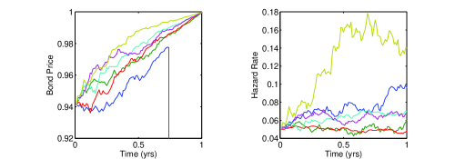
Figure 1: Sample paths of the defaultable discount bond and the associated hazard rate. We choose $\phi(t)=\mbox{$\rm e$}^{-0.025t}$, and the initial term structure is assumed to be flat so that $P_{0t}=\mbox{$\rm e$}^{-0.02t}$. The information flow rate parameter is set to be $\sigma=0.3$, and the bond maturity is one year.

VI Options on defaultable bonds

We consider the problem of pricing an option on a defaultable bond with bond maturity $T$. Let $K$ be the option strike price and let $t~{}(<T)$ be the option maturity. The payoff of the option is then $(B_{tT}-K)^{+}$. Let us write the bond price at in the form

$$B_{tT}={\mathds{1}}\{\tau>t\}B(t,\xi_{t}),$$ (37)

where the function $B(t,y)$ is defined by

$$B(t,y)=P_{tT}\,\frac{\int^{\infty}_{T}p(u)\exp\left[\sigma\phi(u)y-\frac{1}{2}\sigma^{2}\phi^{2}(u)t\right]\mbox{$\rm d$}u}{\int^{\infty}_{t}p(u)\exp\left[\sigma\phi(u)y-\frac{1}{2}\sigma^{2}\phi^{2}(u)t\right]\mbox{$\rm d$}u}.$$ (38)

We make note of the identity

$$\big{(}{\mathds{1}}\{\tau>t\}B(t,\xi_{t})-K\big{)}^{+}={\mathds{1}}\{\tau>t\}\big{(}B(t,\xi_{t})-K\big{)}^{+},$$ (39)

satisfied by the option payoff. The price of the option is thus given by

$$C_{0}=P_{0t}\,{\mathbb{E}}\Big{[}{\mathds{1}}\{\tau>t\}\big{(}B(t,\xi_{t})-K\big{)}^{+}\Big{]}.$$ (40)

We find, in particular, that the option payoff is a function of the random variables $\tau$ and $\xi_{t}$. To determine the expectation (40) we need therefore to work out the joint density of $\tau$ and $\xi_{t}$, defined by

$$\rho(u,y)={\mathbb{E}}\left[\delta(\tau-u)\delta(\xi_{t}-y)\right]=-\frac{\mbox{$\rm d$}}{\mbox{$\rm d$}u}\,{\mathbb{E}}\left[{\mathds{1}}\{\tau>u\}\delta(\xi_{t}-y)\right].$$ (41)

Note that the expression

$$A_{0}(u,y)=P_{0t}\,{\mathbb{E}}\left[{\mathds{1}}\{\tau>u\}\delta(\xi_{t}-y)\right]$$ (42)

appearing on the right side of (41), with an additional discounting factor, can be regarded as representing the price of a “defaultable Arrow-Debreu security” based on the value at time $t$ of the information process.

To work out the expectation appearing here we shall use the Fourier representation for the delta function:

$$\delta(\xi_{t}-y)=\frac{1}{2\pi}\int_{-\infty}^{\infty}\exp\left(-\mbox{$\rm i$}y\lambda+\mbox{$\rm i$}\xi_{t}\lambda\right)\mbox{$\rm d$}\lambda,$$ (43)

which of course has to be interpreted in an appropriate way with respect to integration against a class of test functions. We have

$$\mathbb{E}\left[{\mathds{1}}\{\tau>u\}\delta(\xi_{t}-y)\right]=\frac{1}{2\pi}\int_{-\infty}^{\infty}\mbox{$\rm e$}^{-{\rm i}y\lambda}\mathbb{E}\left[{\mathds{1}}\{\tau>u\}\mbox{$\rm e$}^{{\rm i}\xi_{t}\lambda}\right]\mbox{$\rm d$}\lambda.$$ (44)

The expectation appearing in the integrand is given by

$$\mathbb{E}\left[{\mathds{1}}\{\tau>u\}\mbox{$\rm e$}^{{\rm i}\xi_{t}\lambda}\right]=\int_{-\infty}^{\infty}{\mathds{1}}\{x>u\}\,p(x)\exp\left(\mbox{$\rm i$}\sigma\lambda t\phi(x)-\mbox{$\textstyle\frac{1}{2}$}\lambda^{2}t\right)\mbox{$\rm d$}x,$$ (45)

where we have made use of the fact that the random variables $\tau$ and $B_{t}$ appearing in the definition of the information process (33) are independent. We insert this intermediate result in (44) and rearrange terms to obtain

$$\mathbb{E}\left[{\mathds{1}}\{\tau>u\}\delta(\xi_{t}-y)\right]=\frac{1}{2\pi}\int_{-\infty}^{\infty}\!\!\!{\mathds{1}}\{x>u\}\,p(x)\!\int_{-\infty}^{\infty}\!\!\mbox{$\rm e$}^{-{\rm i}y\lambda+{\rm i}\sigma\lambda t\phi(x)-\frac{1}{2}\lambda^{2}t}\mbox{$\rm d$}\lambda\mbox{$\rm d$}x.$$ (46)

Performing the Gaussian integration associated with the $\lambda$ variable we deduce that the price of the defaultable Arrow-Debreu security is

$$A_{0}(u,y)=\frac{P_{0t}}{\sqrt{2\pi\,t}}\int_{-\infty}^{\infty}{\mathds{1}}\{x>u\}p(x)\exp\left[-\frac{(\sigma t\phi(x)-y)^{2}}{2t}\right]\mbox{$\rm d$}x.$$ (47)

For the calculation of the price of a call option written on a defaultable discount bond, it is convenient to rewrite (47) in the following form:

$$A_{0}(y)=\frac{P_{0t}}{\sqrt{2\pi\,t}}\exp\left(-\frac{y^{2}}{2t}\right)\int_{u}^{\infty}p(x)\exp\left(\sigma\phi(x)y-\mbox{$\textstyle\frac{1}{2}$}\,\sigma^{2}\phi^{2}(x)t\right)\mbox{$\rm d$}x.$$ (48)

It follows that for the joint density function we have

$$\rho(u,y)=\frac{1}{\sqrt{2\pi t}}\,p(u)\,\mbox{$\rm e$}^{-\frac{1}{2t}y^{2}}\,\mbox{$\rm e$}^{\sigma\phi(u)y-\frac{1}{2}\,\sigma^{2}\phi^{2}(u)t}.$$ (49)

The price of the call option can therefore be worked out as follows:

$$C_{0} = P_{0t}\int_{-\infty}^{\infty}\mbox{$\rm d$}u\int_{-\infty}^{\infty}\mbox{$\rm d$}y\,\rho(u,y){\mathds{1}}\{u>t\}(B(t,y)-K)^{+}$$ (50)

$$= \frac{P_{0t}}{\sqrt{2\pi t}}\int_{-\infty}^{\infty}\!\!\!\mbox{$\rm d$}y\,\mbox{$\rm e$}^{-\frac{1}{2t}y^{2}}(B(t,y)-K)^{+}\left[\int_{t}^{\infty}p(u)\mbox{$\rm e$}^{\sigma\phi(u)y-\frac{1}{2}\sigma^{2}\phi^{2}(u)t}\mbox{$\rm d$}u\right].\,\,\,\,$$

We notice that the term inside the square brackets is identical to the denominator of the expression for $B(t,y)$. Therefore, we have

$$C_{0} = \frac{P_{0t}}{\sqrt{2\pi t}}\int_{-\infty}^{\infty}\!\!\!\mbox{$\rm d$}y\,\mbox{$\rm e$}^{-\frac{1}{2t}y^{2}}\left(P_{tT}\int_{T}^{\infty}p(u)\mbox{$\rm e$}^{\sigma\phi(u)y-\frac{1}{2}\sigma^{2}\phi^{2}(u)t}\mbox{$\rm d$}u\right.$$ (51)

$$\qquad\qquad\qquad\qquad\qquad\left.-K\int_{t}^{\infty}p(u)\mbox{$\rm e$}^{\sigma\phi(u)y-\frac{1}{2}\sigma^{2}\phi^{2}(u)t}\mbox{$\rm d$}u\right)^{+}.$$

An analysis similar to the one carried out in Brody & Friedman (2009) shows the following result: Provided that $\phi(u)$ is a decreasing function there exists a unique critical value $y^{*}$ for $y$ such that

$$P_{tT}\int_{T}^{\infty}p(u)\mbox{$\rm e$}^{\sigma\phi(u)y-\frac{1}{2}\sigma^{2}\phi^{2}(u)t}\mbox{$\rm d$}u-K\int_{t}^{\infty}p(u)\mbox{$\rm e$}^{\sigma\phi(u)y-\frac{1}{2}\sigma^{2}\phi^{2}(u)t}\mbox{$\rm d$}u>0$$ (52)

if $y<y^{*}$. On the other hand, if $\phi(u)$ is increasing, then there is likewise a unique critical value $y^{\dagger}$ of $y$ such that for $y>y^{\dagger}$ we have

$$P_{tT}\int_{T}^{\infty}p(u)\mbox{$\rm e$}^{\sigma\phi(u)y-\frac{1}{2}\sigma^{2}\phi^{2}(u)t}\mbox{$\rm d$}u-K\int_{t}^{\infty}p(u)\mbox{$\rm e$}^{\sigma\phi(u)y-\frac{1}{2}\sigma^{2}\phi^{2}(u)t}\mbox{$\rm d$}u>0.$$ (53)

Therefore, we can perform the $y$-integration in (51) to obtain the value

$$C_{0} = P_{0T}\int_{T}^{\infty}p(u)\,N\left(\frac{y^{*}-\sigma\phi(u)t}{\sqrt{t}}\right)\mbox{$\rm d$}u$$ (54)

$$\qquad\qquad-P_{0t}K\int_{t}^{\infty}p(u)\,N\left(\frac{y^{*}-\sigma\phi(u)t}{\sqrt{t}}\right)\mbox{$\rm d$}u$$

when $\phi(u)$ is decreasing. If $\phi(u)$ is increasing, we have

$$C_{0} = P_{0T}\int_{T}^{\infty}p(u)\,N\left(\frac{\sigma\phi(u)t-y^{\dagger}}{\sqrt{t}}\right)\mbox{$\rm d$}u$$ (55)

$$\qquad\qquad-P_{0t}K\int_{t}^{\infty}p(u)\,N\left(\frac{\sigma\phi(u)t-y^{\dagger}}{\sqrt{t}}\right)\mbox{$\rm d$}u.$$

The critical values $y_{\phi}^{*}(t,T,K,\sigma)$ and $y_{\phi}^{\dagger}(t,T,K,\sigma)$ can be determined numerically to value the prices of call options. An example of the call price as a function of its strike and maturity, when $\phi(u)$ is decreasing, is shown in figure 2. If the function $\phi(u)$ is not monotonic, then there is in general more than one critical value of $y$ for which the argument of the max function in (51) is positive. Therefore, in this case there will be more terms in the option-valuation formula.

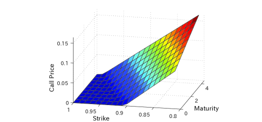
Figure 2: Price of a call option on a defaultable discount bond. The bond maturity is five years. The information-adjusting function is set to be $\phi(t)=\mbox{$\rm e$}^{-0.05t}$, and the initial term structure is assumed to be flat so that $P_{0t}=\mbox{$\rm e$}^{-0.02t}$. The information flow rate is set to be $\sigma=0.25$.

The case represented by a simple discount bond is merely an example and as such cannot be taken too seriously as a realistic model. Nevertheless it is interesting that modelling the information available about the default time leads to a dynamical model for the bond price, in which the Brownian fluctuations driving the price process arise in a natural way as the innovations associated with the flow of information to the market concerning the default time. Thus no “background filtration” is required for the analysis of default in models here proposed. The information flow-rate parameter $\sigma$ is not directly observable, but rather can be backed out from option-price data on an “implied” basis. The extension of the present investigation, which can be regarded as a synthesis of the “density” approach to interest-rate modelling proposed in Brody & Hughston (2001, 2002) and the information-based asset pricing framework developed in Brody, Hughston & Macrina (2007, 2008a, 2008b) and Macrina (2006), to multiple asset situations with portfolio credit risk will be pursued elsewhere.

References

- (1) Bielecki, T. R., Jeanblanc, M. & Rutkowski, M. (2009) Credit Risk Modelling (Osaka University Press).
- (2) Brody, D. C., Brody, J., Meister, B. K. & Parry, M. F. (2010) Outsider trading. arXiv:1003.0764.
- (3) Brody, D. C., Davis, M., H., A., Friedman, R. L. & Hughston, L. P. (2008) Informed traders. Proceedings of the Royal Society London A465, 1103 1122.
- (4) Brody, D. C. & Friedman, R. L. (2009) Information of Interest. Risk Magazine, December 2009 issue, 101-106.
- (5) Brody, D. C. & Hughston, L. P. (2001) Interest rates and information geometry. Proceedings of the Royal Society London A457, 1343-1364.
- (6) Brody, D. C. & Hughston, L. P. (2002) Entropy and information in the interest rate term structure. Quantitative Finance 2, 70-80.
- (7) Brody, D. C., Hughston, L. P. & Macrina, A. (2007) Beyond hazard rates: a new framework for credit-risk modelling. In Advances in Mathematical Finance: Festschrift Volume in Honour of Dilip Madan (Basel: Birkhäuser).
- (8) Brody, D. C., Hughston, L. P. & Macrina, A. (2008a) Information-based asset pricing. International Journal of Theoretical and Applied Finance 11, 107-142.
- (9) Brody, D. C., Hughston, L. P. & Macrina, A. (2008b) Dam rain and cumulative gain. Proceedings of the Royal Society London A464, 1801-1822.
- (10) Brody, D. C., Hughston, L. P. & Macrina, A. (2010) Modelling information flows in financial markets. In Advanced Mathematical Methods for Finance, G. Di Nunno & B. Øksendal, eds. (Berlin: Springer-Verlag).
- (11) Çetin, U., Jarrow, R., Protter, P. & Yildirim, Y. (2004) Modeling credit risk with partial information. Annals of Applied Probability 14, 11-67-1178.
- (12) Coculescu, D., Geman, H. & Jeanblanc, M. (2008) Valuation of default sensitive claims under inperfect information. Finance and Stochastics 12, 195-218.
- (13) Duffie, D. & Lando, D. (2001) Term structures of credit spreads with incomplete accounting information. Econometrica 69, 633-664.
- (14) Föllmer, H., Wu, C.-T. & Yor, M. (1999) Canonical decomposition of linear transformations of two independent Brownian motions motivated by models of insider trading. Stochastic Processes and their Applications 84, 137-164.
- (15) Frey, R. & Schmidt, T. (2009) Pricing corporate securities under noisy asset information. Mathematical Finance 19, 403-421.
- (16) Geman, H., Madan, D. B. & Yor, M. (2007) Probing option prices for information. Methodology and Computing in Applied Probability 9, 115-131.
- (17) Giesecke, K. (2006) Default and information. Journal of Economic Dynamics and Control 30, 2281-2303.
- (18) Hoyle, E., Hughston, L. P. & Macrina, A. (2009) Levy random bridges and the modelling of financial information. arXiv:0912.3652.
- (19) Hoyle, E., Hughston, L. P. & Macrina, A. (2010) Stable-1/2 bridges and insurance: a Bayesian approach to non-life reserving. arXiv:1005.0496.
- (20) Hughston, L. P. & Macrina, A. (2009) Pricing fixed-income securities in an information-based framework. arXiv:0911.1610.
- (21) Jarrow, R. & Protter, P. (2004) Structural versus reduced-form models: a new information based perspective. Journal of Investment and Management 2, 1-10.
- (22) Kusuoka, S. (1999) A remark on default risk models. Advances in Mathematical Economics 1, 69-82.
- (23) Macrina, A. (2006) An information-based framework for asset pricing: -factor theory and its applications. PhD thesis, King’s College London.
- (24) Macrina, A. & Parbhoo, P. A. (2010) Security pricing with information-sensitive discounting. In Recent Advances in Financial Engineering 2009: Proceedings of the KIER-TMU International Workshop on Financial Engineering 2009 (Singapore: World Scientific).
- (25) Rutkowski, M. & Yu, N. (2007) On the Brody-Hughston-Macrina approach to modelling of defaultable term structure. International Journal of Theoretical and Applied Finance 10, 557-589.