TU-868
Tau polarization measurements at the LHC in supersymmetric models with a long-lived stau
Ryuichiro Kitano and Mitsutoshi Nakamura
Department of Physics, Tohoku University, Sendai 980-8578, Japan
Supersymmetry (SUSY) with a long-lived stau is an attractive scenario in the LHC experiments because one can directly observe stau tracks in each SUSY event, and thus precise measurements of SUSY particle masses are possible. In this scenario, we discuss the possibility to observe/measure parity violation in interactions among SUSY particles. Such a measurement will be important in determining spins and chiralities of SUSY particles. We use the last step of the cascade-decay chain: , where the polarization of the tau lepton can be determined statistically by looking at the energy distribution of the final state lepton. Comparing with the theoretical formula of the neutralino differential decay width, one can extract the size of parity violation in the interaction vertices among the stau, the tau lepton and the neutralino. We perform a Monte Carlo simulation to see if the effect is visible at the LHC experiments.
1 Introduction
If supersymmetry (SUSY) is the solution to the hierarchy problem, the superpartners should weigh around a few hundred GeV to TeV energy range, which is accessible at the LHC experiments. The way to discover SUSY or to measure the properties of SUSY particles are quite different depending on the pattern of the superparticle spectrum. In particular, the property of the lightest SUSY particle (LSP) is important for the search strategies.
Motivated by an explanation of dark matter of the Universe, many collider studies of SUSY models have assumed the case with the LSP being the neutralino (admixture of the Higgsinos and the gauginos). In the neutralino LSP case, the final states of the SUSY events always contain invisible neutralinos, and one needs various measurements to be combined in order to determine sparticle masses. The situation drastically changes if one assumes that one of the charged sleptons is lighter than the lightest neutralino. Such a scenario is possible if the slepton is not absolutely stable. For example, the slepton can decay into a lepton and gravitino if kinematically allowed. In particular, the scalar tau lepton (stau) can easily be lighter than the neutralino in many SUSY models due to the quantum correction through the large Yukawa interaction.
If the life-time of the stau is longer than the time scale of the collider experiments (a few nsec), we will see charged tracks left by staus in each SUSY events, instead of the missing momentum in the neutralino LSP scenario. Methods to search for a long-lived charged particle in hadron colliders have been studied in Refs. [1, 2, 3, 4, 5]. Also, various advantages in studying SUSY models at the LHC have been reported. The stau momenta and velocities can be measured by analyzing the stau tracks, from which the stau mass can be extracted with a good accuracy [6, 7, 8]. The measurements of other sparticle masses [9, 10, 11, 12, 13, 14] and the spin measurement of the stau [15] have also been discussed. Methods to measure the stau life-time have been proposed in various contexts [16, 17, 18, 19, 20]. The chargino-neutralino production and subsequent decay processes at the LHC have been studied in Ref. [21] and the possibilities to observe parity/CP violations have been discussed.
In this paper, we discuss the possibility to measure the tau polarization in the neutralino decay, , where the neutralinos are mainly produced by the cascade decays of colored SUSY particles. The tau polarization carries information on whether the lightest stau is the partner of the right- or left-handed tau lepton, and also whether the decaying neutralino is mainly composed of the gauginos or the Higgsinos. The polarization can be determined by looking at the energy distribution of the -decay product [22] due to the fact that the weak interaction maximally violates parity. We use the leptonic decay mode of the tau lepton, , in this work. We first show the formula for the lepton-energy distribution in the neutralino decay, and by using it we fit the data from the Monte Carlo simulation. We find that the size of parity violation (the tau polarization) can be measured in a simple model where only one of the neutralinos contributes to the final state. In a more complicated case, where there are two neutralinos contribute to the same final state, we can correctly reproduce the signs of parity violation in each decay vertex.
2 Neutralino decay
In this section, we present the differential decay width of as a function of the lepton-energy fraction. The parity asymmetry of this decay process carries information on the chirality of the stau and the composition of the neutralino, i.e., whether it is gaugino-like or Higgsino-like.
The measurement of the tau polarization has also been studied in the neutralino LSP case. The effects of the tau polarization in the di-tau invariant mass distribution in cascade decays were studied in Refs. [23, 24, 25]. Ref. [26] studied the distribution of the softest -jets to extract the tau polarization in the co-annihilation region in the mSUGRA model. The tau polarization measurements at colliders were studied in the stau-pair productions in Refs. [27, 28, 29]. The measurements of CP violation at colliders were also studied in Refs. [30, 31, 32].
2.1 Decay width
The polarization information of the tau lepton is imprinted to the energy distribution of the lepton in the leptonic tau decay. We show in this subsection the formula for the distribution of the lepton-energy fraction in the neutralino decays.
The relevant interaction Lagrangian for the neutralino decay is
| (1) |
where and are the chirality projection operators, and and are coupling constants. We will discuss the relation to the underlying model parameters in the next subsection. The tau lepton is polarized if there is parity violation, i.e., . The explicit calculation shows that the differential decay width of the process, , is
| (2) |
where is the partial decay width of the leptonic mode [22]. The variable is the lepton-energy fraction:
| (3) |
where the energy of the lepton and ( and ) are those in the rest frame of . The formula (2) is independent of the tau charge or the flavor of the final state lepton, i.e., electron or muon. The parameter represents the tau polarization and it is expressed in terms of the Lagrangian parameters:
| (4) |
The distributions in Eq. (2) for are shown in the left panel of Fig. 1. The value corresponds to the decay into right (left) handed . The lepton tends to be emitted to the same direction of if (left-handed ).


2.2 Coupling constants and the model parameters
The coupling constants in Eq. (1) are expressed in terms of the neutralino- and the stau-mixing parameters as follows:
| (5) | ||||
| (6) |
where is the coupling constant of the gauge interaction, is that of , is the ratio of the two vacuum expectation values (VEV) of the Higgs fields and is the VEV of the Higgs field:
| (7) | |||
| (8) |
The matrix elements are those of a unitary matrix which diagonalizes the neutralino mass matrix,
| (9) |
such that
| (10) |
The mixing angle of the stau is defined by
| (11) |
For example, let us consider the case in which the lightest neutralino () and the lightest stau () are mainly the Bino and , respectively, i.e., and . In this case, the largest contribution to the decay is the second term in Eq. (6). Therefore, the parity violation parameter in Eq. (2) is .
In the case where the decaying neutralino is mainly the Wino and the lightest stau is , the situation is different. Since the pure Wino does not couple to the right-handed stau, the decay occurs either through the neutralino mixing or the stau mixing. In both cases, the parity violation is in contrast to the previous example.
3 Monte Carlo simulation
In this section, we demonstrate by using a Monte Carlo simulation that the distribution obtained in the previous section is observable at the LHC experiments.
3.1 Basic set up
We generated events of SUSY particle productions at a collider at TeV (LHC) by using the HERWIG package [33]. We use CTEQ5L [34] for the parton distribution function. The TAUOLA package [35] is used for the decays and the events are passed through the AcerDET detector simulator [36] where the lepton momentum are smeared to simulate the detector effects.
The final state contains two stau tracks. The identification of those staus can be used to eliminate the background from the Standard Model processes. In order to distinguish staus from muons, we impose following selection cuts on the candidate stau tracks:
-
•
,
-
•
GeV ,
-
•
.
Here and hereafter, we do not take into account the momentum and the velocity resolutions of the staus, i.e., the parton level information is used. We assume in the following that the stau and neutralino masses are known. It has been reported in Refs. [7, 8, 9, 10, 11, 14] that those quantities are measurable with a good accuracy.
3.2 Lepton cut and the deformation of the distribution
We also require for the lepton momentum. This cut affects the shape of the distribution in Eq. (2). We model the effect of the cut in the distribution by multiplying the following weight:
| (12) |
where is 15 GeV, and and are parameters to be determined by fitting the data. We plot in the right panel of Fig. 1 the distribution after multiplying this factor with and .
3.3 Model I
We use the MSSM without flavor mixing and ignore the Yukawa interactions of the first and second generations. As the first example, we take a simple model in which only one of the neutralinos () and one of the staus are significantly lighter than others, and the lightest neutralino and the lightest stau are almost the Bino and right-handed, respectively. The value of the parity violation parameter is
| (13) |
in this case.
The MSSM parameters we take are listed in Tab. 1. We follow the convention of SUSY Les Houches Accord [37]. The and masses are calculated to be
| (14) |
We used the ISAJET package [38] for the calculation of the mass spectrum and the branching ratios. We generate 10,000 SUSY events with the parameter set given in Tab. 1. The number of events corresponds to the integrated luminosity of 14.5 .
| Parameter | Value |
|---|---|
| [GeV] | |
| [GeV] | |
| [GeV] | |
| [GeV] | |
| [GeV] | |
| [GeV] | |
| [GeV] | |
| [GeV] | |
| [GeV] | |
| [GeV] | |
| [GeV] | |
| [GeV] | |
| [GeV] | |
| [GeV] | |
| [GeV] | |
| [GeV] | |
| [GeV] | |
| [GeV] | |
| [GeV] | |
| [GeV] | |
| [GeV] |
The neutralinos are mainly produced by the cascade decays of the squarks and gluinos. The value of (the lepton-energy fraction) in each candidate event can be calculated from the measured invariant mass of the lepton and the stau,
| (15) |
where is
| (16) |

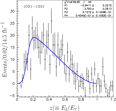
We show in Fig. 2 the histograms of the invariant mass (left) and the parameter (right). In these plots, we select all possible combinations of a stau and a lepton with the opposite charges in each candidate event. In order to eliminate the contributions from wrong combinations and from background events such as leptons from -boson decays, we subtract the same distributions calculated by using the combinations with the same signs [14]. After the selection cuts and the charge subtraction explained above, 978 events remained.
3.4 Model II
As the second example, we take a model where the Wino-like neutralino is not so heavy compared to the Bino-like one as is so in the models motivated by the GUT relation of the gaugino masses. The model parameters are listed in Tab. 2. The neutralino and stau masses are
| (18) |
The parity asymmetries and are calculated to be
| (19) |
Unlike the case of Model I, we cannot reconstruct in the event-by-event basis since we do not know whether the decaying neutralino is or . Therefore, we need to directly fit the invariant mass distribution which contains events of both neutralinos.
| Parameter | Value |
|---|---|
| [GeV] | |
| [GeV] | |
| [GeV] | |
| [GeV] | |
| [GeV] | |
| [GeV] | |
| [GeV] | |
| [GeV] | |
| [GeV] | |
| [GeV] | |
| [GeV] | |
| [GeV] | |
| [GeV] | |
| [GeV] | |
| [GeV] | |
| [GeV] | |
| [GeV] | |
| [GeV] | |
| [GeV] | |
| [GeV] | |
| [GeV] |
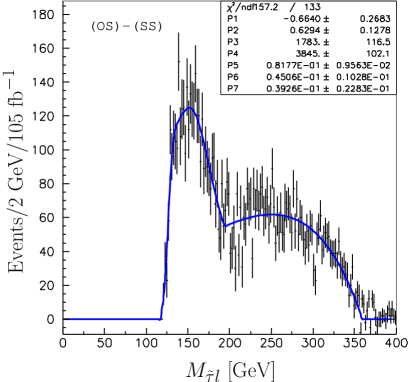
We generated 90,000 SUSY events with this parameter set. The number of events corresponds to the integrated luminosity of 104.6 . We show the invariant mass distributions (Fig. 3) using the same technique as we used for the Model I. After the cuts and the subtraction explained before, 7,677 events remained. We can see contributions from decays of two kinds of neutralinos.
Before fitting the distribution in Fig. 3, we checked the validity of Eq. (2) combined with Eq. (12) for the Model II. We did it by separating the and the events by using information from the event generator and performed the fitting for each event set. Reasonable values for and are obtained:
| (20) |
For the fitting of the histogram in Fig. 3, we use the sum of two fitting functions corresponding to each neutralino:
| (21) |
where , and is the function in Eq. (2). The energy fraction is related to the - invariant mass, , as
| (22) |
There are eight fitting parameters , , and for in the function.
Since it is difficult to find the best fit for such many parameters, we here make a (semi) theoretic assumption on a relationship between two parameters and in order to reduce the number of parameters. In Eq. (21), the combinations of represent the average values of from the decay in the laboratory frame. Since the neutralinos are produced mainly from heavy colored particles, it is likely to be highly boosted and thus the tau lepton from the neutralino decay is pointing to the similar direction to the one of the neutralino in the laboratory frame. Therefore, there is an approximate relation:
| (23) |
where is
| (24) |
The average transverse momentum of the neutralino, , is independent of the neutralino mass if it is highly boosted. Therefore, the ratio of is estimated to be
| (25) |
By imposing the above relation, we could fit with the function in Eq. (21):
| (26) |
We obtain the correct signs for each parity violation although the magnitude of the parity violation is obtained to be smaller than the theoretical input values ( and , respectively) due to our simple ansatz on the fitting function.
4 Summary
We studied the polarization measurement of the tau lepton at the LHC in the long-lived stau scenario. The polarization of the tau lepton from the neutralino decays carries information on whether the neutralino is Higgsino-like or gaugino-like and the chirality of the partner of the stau.
We have shown that the polarization can be measured by fitting the distribution of the lepton-energy fraction () in the leptonic decays. We performed Monte Carlo simulations for two parameter sets of the MSSM. The first example we took is a simple case where the Bino-like neutralino is significantly lighter than others. In this case, we can directly fit the energy fraction by the theoretical function and the parity violation can be measured successfully.
In the second case where the Wino-like neutralino also contributes to the same final state, we fit the - invariant mass distribution with the two contributions summed. Although the fitting gives a milder asymmetry compared to the theoretical inputs, we can obtain qualitatively correct features of parity violation in each neutralino decay.
Acknowledgements
We would like to thank T. Moroi and T. Ito for useful discussions. RK is supported in part by the Grant-in-Aid for Scientific Research 21840006 of JSPS.
References
- [1] M. Drees and X. Tata, Phys. Lett. B 252, 695 (1990).
- [2] J. L. Feng and T. Moroi, Phys. Rev. D 58, 035001 (1998) [arXiv:hep-ph/9712499].
- [3] S. P. Martin and J. D. Wells, Phys. Rev. D 59, 035008 (1999) [arXiv:hep-ph/9805289].
- [4] S. Dimopoulos, S. D. Thomas and J. D. Wells, Nucl. Phys. B 488, 39 (1997) [arXiv:hep-ph/9609434].
- [5] A. Nisati, S. Petrarca, and G. Salvini, Mod. Phys. Lett. A12, 2213 (1997), arXiv:hep-ph/9707376.
- [6] G. Polesello and A. Rimoldi, ATLAS Internal Note ATL-MUON-99-006.
- [7] S. Ambrosanio, B. Mele, S. Petrarca, G. Polesello, and A. Rimoldi, JHEP 01, 014 (2001), arXiv:hep-ph/0010081.
- [8] J. Ellis, A. R. Raklev and O. K. Oye, ATLAS Note ATL-PHYS-PUB-2007-016; ATLCOM- PHYS-2006-093.
- [9] I. Hinchliffe and F. E. Paige, Phys. Rev. D60, 095002 (1999), arXiv:hep-ph/9812233.
- [10] J. R. Ellis, A. R. Raklev, and O. K. Oye, JHEP 10, 061 (2006), arXiv:hep-ph/0607261.
- [11] M. Ibe and R. Kitano, JHEP 08, 016 (2007), arXiv:0705.3686 [hep-ph].
- [12] J. L. Feng, S. T. French, C. G. Lester, Y. Nir and Y. Shadmi, Phys. Rev. D 80, 114004 (2009) [arXiv:0906.4215 [hep-ph]].
- [13] J. L. Feng et al., arXiv:0910.1618 [hep-ph].
- [14] T. Ito, R. Kitano, and T. Moroi, (2009), arXiv:0910.5853 [hep-ph].
- [15] A. Rajaraman and B. T. Smith, Phys. Rev. D76, 115004 (2007), arXiv:0708.3100 [hep-ph].
- [16] W. Buchmuller, K. Hamaguchi, M. Ratz and T. Yanagida, Phys. Lett. B 588, 90 (2004), arXiv:hep-ph/0402179.
- [17] K. Hamaguchi, Y. Kuno, T. Nakaya and M. M. Nojiri, Phys. Rev. D 70, 115007 (2004), arXiv:hep-ph/0409248.
- [18] J. L. Feng and B. T. Smith, Phys. Rev. D 71, 015004 (2005) [Erratum-ibid. D 71, 019904 (2005)] arXiv:hep-ph/0409278.
- [19] K. Ishiwata, T. Ito and T. Moroi, Phys. Lett. B 669, 28 (2008), arXiv:0807.0975 [hep-ph].
- [20] S. Asai, K. Hamaguchi and S. Shirai, Phys. Rev. Lett. 103, 141803 (2009) [arXiv:0902.3754 [hep-ph]].
- [21] R. Kitano, JHEP 0811, 045 (2008) [arXiv:0806.1057 [hep-ph]].
- [22] B. K. Bullock, K. Hagiwara, and A. D. Martin, Nucl. Phys. B395, 499 (1993).
- [23] S. Y. Choi, K. Hagiwara, Y. G. Kim, K. Mawatari, and P. M. Zerwas, Phys. Lett. B648, 207 (2007), arXiv:hep-ph/0612237; K. Mawatari, (2007), arXiv:0710.4994 [hep-ph].
- [24] M. Graesser and J. Shelton, JHEP 0906, 039 (2009) [arXiv:0811.4445 [hep-ph]].
- [25] T. Nattermann, K. Desch, P. Wienemann, and C. Zendler, JHEP 04, 057 (2009), arXiv:0903.0714 [hep-ph].
- [26] R. M. Godbole, M. Guchait and D. P. Roy, Phys. Rev. D 79, 095015 (2009) [arXiv:0807.2390 [hep-ph]].
- [27] M. M. Nojiri, Phys. Rev. D51, 6281 (1995), arXiv:hep-ph/9412374.
- [28] A. Bartl, H. Eberl, S. Kraml, W. Majerotto and W. Porod, Z. Phys. C 73, 469 (1997) [arXiv:hep-ph/9603410].
- [29] R. M. Godbole, M. Guchait and D. P. Roy, Phys. Lett. B 618, 193 (2005) [arXiv:hep-ph/0411306].
- [30] A. Bartl, T. Kernreiter and O. Kittel, Phys. Lett. B 578, 341 (2004), arXiv:hep-ph/0309340.
- [31] S. Y. Choi, M. Drees, B. Gaissmaier and J. Song, Phys. Rev. D 69, 035008 (2004) arXiv:hep-ph/0310284.
- [32] H. K. Dreiner, O. Kittel and A. Marold, arXiv:1001.4714 [hep-ph].
- [33] S. Moretti, K. Odagiri, P. Richardson, M. H. Seymour, and B. R. Webber, JHEP 04, 028 (2002), arXiv:hep-ph/0204123.
- [34] H. L. Lai et al. [CTEQ Collaboration], Eur. Phys. J. C 12, 375 (2000) [arXiv:hep-ph/9903282].
- [35] S. Jadach, Z. Was, R. Decker, and J. H. Kuhn, Comput. Phys. Commun. 76, 361 (1993).
- [36] E. Richter-Was, (2002), arXiv:hep-ph/0207355.
- [37] P. Z. Skands et al., JHEP 0407, 036 (2004) [arXiv:hep-ph/0311123].
- [38] F. E. Paige, S. D. Protopopescu, H. Baer and X. Tata, arXiv:hep-ph/0312045.