Interpreting the 4-index Notation for Hexagonal Systems

Abstract

A four index notation (e.g. $(10\bar{1}1)$) is often used to denote reciprocal lattice vectors or crystal faces of hexagonal crystals. The purposes of this notation have never been fully explained. This note clarifies the underlying mathematics of a symmetric overcomplete basis. This simplifies and improves the usefulness of the notation.

I Introduction

A reciprocal lattice vector (RLV) has the form $\vec{G}=n_{A}\vec{A}+n_{B}\vec{B}+n_{C}\vec{C}$, where $\vec{A},\vec{B},\vec{C}$ are primitive translations of the reciprocal lattice. The integer “indices” $(n_{A},n_{B},n_{C})$ were originally introduced as the Miller indices, which are reciprocals of the intersection points (in units of $a=|\vec{a}|$, etc.), of a crystal lattice plane with the axes along the primitive translation vectors $\vec{a},\vec{b},\vec{c}$ of the direct lattice. The “4-index” notation $(10\bar{1}1)$ in a hexagonal crystal denotes an RLV with $(n_{A},n_{B},n_{C})=(1,0,1)$. The extra, or third, index $(\bar{1}=-1)$ in $(10\bar{1}1)$ is redundant. This index must equal the negative sum of the first two indices. The notation restores symmetry between equivalent directions which is lost if the third index is omitted. This notation has long been used by crystallographers, dating back at least to Fedorov in 1890Fedorov1890 . An extra Miller index is natural in hexagonal symmetry, because, rather than two $ab$-plane axes $\vec{a},\vec{b}$ at 120^∘, the three symmetrical axes $\vec{a}_{1},\vec{a}_{2},\vec{a}_{3}$, shown in Fig. 1, are natural. The plane of atoms intersects all three axes. The reciprocal intersection points $(hki)$ are forced by trigonometry to obey the rule $h+k+i=0$. The proofDonnay1947 is hinted in Fig. 1.

Even before Bragg scattering was observed and explained (1912-13), the mathematical concept of a dual or reciprocal lattice was usedGibbs1901 . After 1912, physicists recognized the RLV as an x-ray momentum transfer. The “indices” which label planes seem secondary unless we are specifically studying an atomic plane. The redundant index may seem only a nuisance. Since the advantages of the 4-index notation are not always understood, it is common to omit the third index, as would be done in crystal systems which lack $120^{\circ}$ rotations. This note is written in the belief that, once the underlying idea is clearly understood, the four index notation is natural. It can be used to some advantage to label RLV’s $(hkil)$ and also to label directions $[stru]$ (called “zones” when the direction perceived as the common axis of a family of planes) in the direct lattice. However, the 4-index labeling of directions $[stru$ that emerges in my analysis makes a subtle improvement over the one in use in electron microscopyEdington1976 . Otte and CrockerOtte1965 discuss notation carefully, but with a different aim.

Here is the main idea. In an hexagonal crystal, define four unit vectors, with the fourth ($\hat{e}_{4}$) pointing along the $c$-axis. The other three lie in the $ab$-plane, at $120^{\circ}$ to each other, as shown in Fig.1. It is conventional to have them point in the directions of primitive translations of the lattice. Then an arbitrary 3-vector $\vec{v}$ is written with four components, as

$$\vec{v}\rightarrow|v\rangle=\left(\begin{array}[]{l}\vec{v}\cdot\hat{e}_{1}\\ \vec{v}\cdot\hat{e}_{2}\\ \vec{v}\cdot\hat{e}_{3}\\ \vec{v}\cdot\hat{e}_{4}\end{array}\right)=\left(\begin{array}[]{l}v_{1}\\ v_{2}\\ v_{3}\\ v_{4}\end{array}\right).$$ (1)

If $\vec{v}$ is a position vector $\vec{R}$ in “real” space, then it can be written as

$$\vec{R}=\left(\begin{array}[]{l}n_{1}a\\ n_{2}a\\ n_{3}a\\ n_{4}c\end{array}\right)\rightarrow[n_{1}n_{2}n_{3}n_{4}],$$ (2)

where the indices $n_{i}$ are dimensionless, and squared brackets conform to the crystallographic convention for directions in coordinate space. If $\vec{R}$ is a translation vector of the lattice, then the indices are integers. If $\vec{v}$ is a vector of the reciprocal lattice $\vec{Q}$, then it can be written

$$\vec{Q}=2\pi\left(\begin{array}[]{l}n_{1}/a\\ n_{2}/a\\ n_{3}/a\\ n_{4}/c\end{array}\right)\rightarrow(n_{1}n_{2}n_{3}n_{4}),$$ (3)

where again the indices are dimensionless, and rounded brackets conform to convention. If $\vec{Q}$ is a translation vector $\vec{G}$ of the reciprocal lattice, then the dimensionless indices are integers, and the shorthand $\vec{G}=(n_{1}n_{2}n_{3}n_{4})$ is common. In this paper, I will stick to a convention that vectors written in column form as in Eqs.(2,3), or in row form with components separated by commas, contain the full dimensioned components, $\vec{v}\cdot\hat{e}_{i}$. Dimensionless abbreviations are never implied except in the index notations $[n_{1}n_{2}n_{3}n_{4}]$ and $(n_{1}n_{2}n_{3}n_{4})$ without commas. The term “index” will always refer to a dimensionless version of a component of a vector.

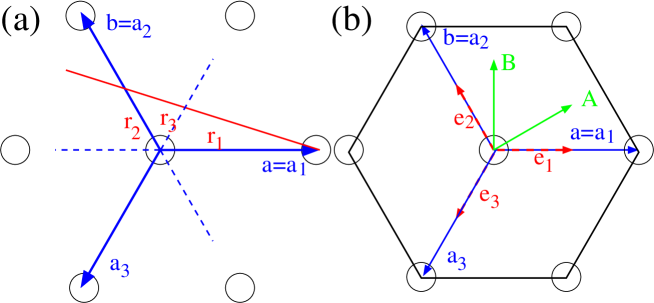
Figure 1: (a) $ab$-plane of a hexagonal crystal, showing $a=a_{1}$ and $b=a_{2}$ axes, the third axis ($a_{3}$). In red is shown the line of intersection of a plane of atoms with the $ab$ plane. This red plane intersects the $a_{1}$ axis at $r_{1}$, the $a_{2}$ axis at $r_{2}$, and the $a_{3}$ axis at $-r_{3}$. It is always possible to choose the origin such that the intersection is at $r_{1}=1$. Then the $120^{\circ}$ geometry guarantees that $1/r_{3}=1/r_{2}+1$. (b) Plaquette of 2-d hexagonal crystal, showing primitive translations $\vec{a},\vec{b}$ of the direct lattice and $\vec{A},\vec{B}$ of the reciprocal lattice.

In Dirac notation, $|v\rangle$ indicates a column vector, while $\langle v|$ indicates a row vector. However, in this paper notation switches between two and three dimensions and between 2-vector, 3-vector and 4-vector systems. The Dirac notation is mostly avoided to reduce ambiguity. When a vector is written alone, it can be assumed a column vector. When written with another vector in a dot product $\vec{u}\cdot\vec{v}$, the left vector is a row vector and the right vector a column vector. When written as a dyad $\vec{v}\vec{v}$, the left vector is a column vector and the right vector a row vector. When written in a line of text with commas, the vector $(a,b,c,d)$ is probably a column vector written sideways to save space.

The 4-vector “basis” is overcomplete. It has both conventional and unconventional features. The basis vectors are, in 4-component notation

$$\hat{e}_{1}\rightarrow\frac{1}{2}\left(\begin{array}[]{r}2\\ -1\\ -1\\ 0\end{array}\right),\ \ \hat{e}_{2}\rightarrow\frac{1}{2}\left(\begin{array}[]{r}-1\\ 2\\ -1\\ 0\end{array}\right),\ \ \hat{e}_{3}\rightarrow\frac{1}{2}\left(\begin{array}[]{r}-1\\ -1\\ 2\\ 0\end{array}\right),\ \ \hat{e}_{4}\rightarrow\left(\begin{array}[]{l}0\\ 0\\ 0\\ 1\end{array}\right).$$ (4)

Note that the sum of the first three indices is always zero, which follows from the fact that the first three unit vectors add to zero, $\hat{e}_{1}+\hat{e}_{2}+\hat{e}_{3}=0$. It is perhaps disconcerting that the unit vectors $\hat{e}_{1},\hat{e}_{2},\hat{e}_{3}$ do not “look like” unit vectors in the 4-vector notation, but this is a consequence of overcompleteness. For example, the second component of the 4-vector that represents $\hat{e}_{1}$, is, according to Eq.(1), $\hat{e}_{1}\cdot\hat{e}_{2}=\cos 120^{\circ}=-1/2$.

The notation makes symmetry explicit. The six translations have their first three indices chosen by the rule, organize three integers chosen from $\pm 1$ and $\pm 2$, in all ways such that they add to zero. Because of the symmetrical mathematics, the scalar product (e.g. $\vec{u}\cdot\vec{v}=u_{x}v_{x}+u_{y}v_{y}+u_{z}v_{z}$) in 4-vector form is simple but unconventional:

$$\vec{u}\cdot\vec{v}=\frac{2}{3}(u_{1}v_{1}+u_{2}v_{2}+u_{3}v_{3})+u_{4}v_{4}.$$ (5)

This can easily be verified, and will be explained in Sec. III.

II Conventional (“bi-orthogonal”) Basis

When one drops the redundant third index from the 4-index notation, the remaining indices express vectors in a non-orthogonal basis. There is perfectly good mathematics behind this, but it hides symmetry and simplicity. In a hexagonal system, these disadvantages are removed by the 4-index system. In systems of lower symmetry, where translation vectors are not at $90^{\circ}$ and $120^{\circ}$ to each other, such simplification is not available. In this section, the mathematics of non-orthogonal basis sets is reviewed.

To simplify, the $c$-direction is now omitted. The discussion thus refers to crystallography of hexagonal crystals in two dimensions. The third dimension returns in Sec. IV. In the 2-d space of the $ab$ plane, any two vectors that are not parallel or antiparallel can be chosen for a basis. The most obvious choices are the primitive translations $\vec{a}$ and $\vec{b}$, or alternately, the primitive translations $\vec{A}$ and $\vec{B}$ of the reciprocal lattice, defined as $\vec{A}=(2\pi/V)\vec{b}\times\vec{c}$, and similarly for $\vec{B}$. $V$ is the volume of the three-dimensional unit cell, $V=(\sqrt{3}/2)a^{2}c$. Then we have the usual vector relations $\vec{A}\cdot\vec{a}=2\pi=\vec{B}\cdot\vec{b}$ and $\vec{A}\cdot\vec{b}=0=\vec{B}\cdot\vec{a}$. These relations indicate that the basis sets $(\vec{a},\vec{b})$ and $(\vec{A},\vec{B})$ are bi-othogonal.

It not always mentioned in texts that the primitive direct lattice vectors and the primitive RLV’s are examples of the mathematical notion of bi-orthogonal basis vectors. The important property is completeness: any vector can be expressed as a unique linear combination $\vec{v}=v_{a}\vec{a}+v_{b}\vec{b}$. Note that $\vec{v}\cdot\vec{a}=v_{a}a^{2}+v_{b}\vec{a}\cdot\vec{b}$, where $\vec{a}\cdot\vec{b}$ equals $-a^{2}/2$ in hexagonal systems. The coefficients $v_{a}$ and $v_{b}$ are found by solving a $2\times 2$ linear system in $\vec{v}\cdot\vec{a}$ and $\vec{v}\cdot\vec{b}$. A nice aspect of bi-orthogonality is that it diagonalizes the $2\times 2$ system and gives simple formulas for the coefficients, namely $v_{a}=\vec{A}\cdot\vec{v}/2\pi$, $v_{b}=\vec{B}\cdot\vec{v}/2\pi$.

It is arbitrary which basis (direct space or reciprocal) is taken to be primary and which to be dual. Thus, an arbitrary vector $\vec{v}$ has an alternate representation, $\vec{v}=v_{A}\vec{A}+v_{B}\vec{B}.$ The coefficients are $v_{A}=\vec{a}\cdot\vec{v}/2\pi$, $v_{B}=\vec{b}\cdot\vec{v}/2\pi$. The inner product $\vec{u}\cdot\vec{v}$ of two vectors is not given simply by $v_{a}^{2}+v_{b}^{2}$, but involves also the cross term $v_{a}v_{b}$. The simple formula is $\vec{u}\cdot\vec{v}=2\pi(u_{A}v_{a}+u_{B}v_{b})$, where the row vector is expressed in the basis dual to the one chosen for the column vector. An equivalent formula is $\vec{u}\cdot\vec{v}=2\pi(u_{a}v_{A}+u_{b}v_{B})$. A compact mathematical representation of these relations is given by the equation $|A\rangle\langle a|+|B\rangle\langle b|=2\pi{\bf{\mathsf{1}}}$, or by the alternate equation $|a\rangle\langle A|+|b\rangle\langle B|=2\pi{\bf{\mathsf{1}}}$. Here the notation $|v\rangle$ means a 2-vector, and ${\bf{\mathsf{1}}}$ is the $2\times 2$ unit matrix. If written as a 2-component column vector, the basis should either be orthonormal, or if non-orthonormal, one has to be careful to use the direct and dual basis for the column vector $|v\rangle$ and the row vector $\langle v|$. In dyad notation, the relations are

$$\vec{A}\vec{a}+\vec{B}\vec{b}=\vec{a}\vec{A}+\vec{b}\vec{B}=2\pi{\bf{\mathsf{1}}}.$$ (6)

This formula is called “the completeness relation” or, equivalently, “the decomposition of unity.” Although this gives elegant formulas for inner products in non-orthogonal basis sets, these formulas are not likely to be used unless the vectors $\vec{u}$ and $\vec{v}$ belong separately, one to direct, and the other to reciprocal space. Then the formulas are obvious. One has no trouble realizing that $\vec{Q}\cdot\vec{r}=(Q_{A}\vec{A}+Q_{B}\vec{B})\cdot(r_{a}\vec{a}+r_{b}\vec{b})$ is equal to $2\pi(Q_{A}r_{a}+Q_{B}r_{b})$.

III Overcomplete symmetrical basis

For two dimensional vectors, or the $ab$-plane components of 3-d vectors of an hexagonal crystal, the overcomplete symmetrical basis is the three vectors $\hat{e}_{1},\hat{e}_{2},\hat{e}_{3}$ which lie at $120^{\circ}$ to each other, as shown in Fig.1. The key relationship is the dyad formula

$$\frac{2}{3}(\hat{e}_{1}\hat{e}_{1}+\hat{e}_{2}\hat{e}_{2}+\hat{e}_{3}\hat{e}_{3})={\bf\mathsf{1}}.$$ (7)

This decomposition of unity is a very nice alternative to Eq.(6). It is no longer necessary to have dual sets of direct and reciprocal lattice vectors. The three vectors $\hat{e}_{i}$ are self-dual. The scalar product of any two 2-vectors can be written as

$$\vec{u}\cdot\vec{v}=\vec{u}\cdot\mathsf{1}\cdot\vec{v}=\frac{2}{3}(\vec{u}\cdot\hat{e}_{1}\hat{e}_{1}\cdot\vec{v}+\vec{u}\cdot\hat{e}_{2}\hat{e}_{2}\cdot\vec{v}+\vec{u}\cdot\hat{e}_{3}\hat{e}_{3}\cdot\vec{v}).$$ (8)

This formula can be written in an overcomplete 3-vector notation as

$$\vec{u}\cdot\vec{v}=\frac{2}{3}(u_{1}v_{1}+u_{2}v_{2}+u_{3}v_{3})=\frac{2}{3}\left(\begin{array}[]{lll}u_{1}&u_{2}&u_{3}\end{array}\right)\left(\begin{array}[]{r}v_{1}\\ v_{2}\\ v_{3}\end{array}\right),$$ (9)

where the usual array multiplication rule is obeyed. Unlike the case of the biorthogonal basis, here there is no need for care about whether $\vec{u}$ or $\vec{v}$ is in direct or reciprocal space, or whether the primary or the dual basis is implied. The formula works for any two vectors.

It is worth emphasizing one subtlety. In the bi-orthogonal basis, when a column vector has indices $[v_{a}v_{b}]$, this means that $\vec{v}=v_{a}\vec{a}+v_{b}\vec{b}$, even though $v_{a}\neq\vec{v}\cdot\vec{a}$. Similarly, if the indices are written $(v_{A}v_{B})$, this indicates a vector $\vec{v}=v_{A}\vec{A}+v_{B}\vec{B}$. Very different relations hold true in the symmetric overcomplete basis. If the vector has components $v_{1},v_{2},v_{3}$, this means that $v_{1}=\vec{v}\cdot\hat{e}_{1}$, etc., even though $\vec{v}\neq v_{1}\hat{e}_{1}+v_{2}\hat{e}_{2}+v_{3}\hat{e}_{3}$. The actual answer is $\vec{v}=(2/3)(v_{1}\hat{e}_{1}+v_{2}\hat{e}_{2}+v_{3}\hat{e}_{3})$. This follows immediately from Eq.(7). It does not matter whether the vector $\vec{v}$ is in direct space and indexed as $[v_{1}v_{2}v_{3}]$ or in reciprocal space and indexed as $(v_{1}v_{2}v_{3})$.

Now let us express the reciprocal lattice vectors in the overcomplete symmetric notation. First, recall that since $\vec{A}\cdot\vec{a}=(\sqrt{3}/2)|\vec{A}|a=2\pi$, we have $|\vec{A}|=(2/\sqrt{3})(2\pi/a)$. Then we find $\vec{A}\cdot\hat{e}_{1}=(\sqrt{3}/2)|\vec{A}|=2\pi/a$, $\vec{A}\cdot\hat{e}_{2}=0$, and $\vec{A}\cdot\hat{e}_{3}=-2\pi/a$. Therefore we have

$$\vec{A}_{1}=\vec{A}=\frac{2\pi}{a}\left(\begin{array}[]{r}1\\ 0\\ -1\end{array}\right),\ \ \vec{A}_{2}=\vec{B}=\frac{2\pi}{a}\left(\begin{array}[]{r}0\\ 1\\ -1\end{array}\right),\ \ \vec{A}_{3}=\vec{B}-\vec{A}=\frac{2\pi}{a}\left(\begin{array}[]{r}-1\\ 1\\ 0\end{array}\right).$$ (10)

The set of six symmetry-related smallest RLV’s $(hki)$ are simply all permutations of the three indices $1,0,-1$. The general reciprocal lattice vector is written in various ways, as

$$\vec{G}=n_{A}\vec{A}+n_{B}\vec{B}\rightarrow(n_{A}n_{B}),$$ (11)

$$\vec{G}\rightarrow\frac{2\pi}{a}\left[n_{A}\left(\begin{array}[]{r}1\\ 0\\ \bar{1}\end{array}\right)+n_{B}\left(\begin{array}[]{r}0\\ 1\\ \bar{1}\end{array}\right)\right]=\frac{2\pi}{a}\left(\begin{array}[]{c}n_{A}\\ n_{B}\\ -n_{A}-n_{B}\end{array}\right)\rightarrow(n_{A}n_{B}\ \overline{n_{A}+n_{B}}).$$ (12)

It is amazing how similar the bi-orthogonal representation (Eq.11) is to the overcomplete symmetric representation (Eq.12) for RLV’s. They involve different coordinate systems and rules, yet the former derives from the latter by just dropping the extra third index, and the latter from the former by adding an index which is the negative sum of the first two indices.

The additional advantages of the extra index representation are that it is completely explicit (if $2\pi/a$ is included, the vector is completely specified), and there is no ambiguity about the direct versus dual parts of the bi-orthogonal representation.

IV Conclusions

It is best to think of Eq.(1) as a way of representing the vector $\vec{v}$ but not to think of the components of the 4-vector as if they had meaning similar to the ordinary 3-component notation. In ordinary vector notation, if the vector $\vec{v}$ is denoted $[v_{a}v_{b}v_{c}]$, then it has the formula $v_{a}\vec{a}+v_{b}\vec{b}+v_{c}\vec{c}$. Or, if it is denoted by $(v_{A}v_{B}v_{C})$, then it has the formula $v_{A}\vec{A}+v_{B}\vec{B}+v_{C}\vec{C}$. In 4-index notation, vectors indexed as $(n_{1}n_{2}n_{3}n_{4})$ or $[n_{1}n_{2}n_{3}n_{4}]$ have the formulas

$$\vec{u}=(n_{1}n_{2}n_{3}n_{4})=2\pi\left(\begin{array}[]{r}n_{1}/a\\ n_{2}/a\\ n_{3}/a\\ n_{4}/c\end{array}\right)\rightarrow 2\pi\left(\frac{2}{3a}[n_{1}\hat{e}_{1}+n_{2}\hat{e}_{2}+n_{3}\hat{e}_{3}]+\frac{1}{c}n_{4}\hat{e}_{4}\right).$$ (13)

$$\vec{v}=[n_{1}n_{2}n_{3}n_{4}]=\left(\begin{array}[]{r}n_{1}a\\ n_{2}a\\ n_{3}a\\ n_{4}c\end{array}\right)\rightarrow\left(\frac{2a}{3}[n_{1}\hat{e}_{1}+n_{2}\hat{e}_{2}+n_{3}\hat{e}_{3}]+cn_{4}\hat{e}_{4}\right).$$ (14)

Note the unconventional factor 2/3. When written as an additive sum of primitive vectors proportional to $\hat{e}_{i}$, an arbitrary additive constant can be added to $u_{1},u_{2},u_{3}$ or $v_{1},v_{2},v_{3}$ with no algebraic or notational error. For example,

$$\vec{v}=\frac{2a}{3}[(v_{1}+C)\hat{e}_{1}+(v_{2}+C)\hat{e}_{2}+(v_{3}+C)\hat{e}_{3}]+v_{4}c\hat{e}_{4}\neq\left(\begin{array}[]{c}(v_{1}+C)a\\ (v_{2}+C)a\\ (v_{3}+C)a\\ v_{4}c\end{array}\right)$$ (15)

When written in overcomplete 4-vector notation, $v_{1},v_{2},v_{3}$ are fixed numbers, necessarily adding to zero, and therefore with no arbitrariness. The constant $C$ cannot be added, even though the vector relation $C(\hat{e}_{1}+\hat{e}_{2}+\hat{e}_{3})=0$ is true.

The inner product of two vectors, in 4-vector notation, is

$$\vec{u}\cdot\vec{v}=\left(\begin{array}[]{llll}u_{1},&u_{2},&u_{3},&u_{4}\end{array}\right)\left(\begin{array}[]{rrrr}2/3&0&0&0\\ 0&2/3&0&0\\ 0&0&2/3&0\\ 0&0&0&1\end{array}\right)\left(\begin{array}[]{r}v_{1}\\ v_{2}\\ v_{3}\\ v_{4}\end{array}\right),$$ (16)

This is just an alternative way of writing Eq.(5), that emphasizes the unconventional metric. A factor $2/3$ occurs in the first three diagonal entries. The metric is positive, so the inner product is safely defined. Eq.(16) holds for all vectors provided the indices $u_{i}$ and $v_{i}$ are written in full rather than abbreviated index form. For the special case where one of $\vec{u},\vec{v}$ is in direct and the other in reciprocal space, the inner product, modulo $2\pi$, also has this form, i.e. $(hkil)\cdot[stru]=2\pi[(2/3)(hs+kt+ir)+lu]$, in the index form. If both are direct or reciprocal space vectors, an extra factor $(c/a)^{2}$ or $(a/c)^{2}$ appears in the fourth term.

The unconventional metric with the factor $2/3$ does not appear in previous literature. If the 4-index notation is confined to indexes of planes and reciprocal lattice vectors, then the current definition Eq.(1) agrees with the one in the literature. It is less common for a 4-index notation to be used for coordinate space directions. Inner products are seldom discussed, and the factor $2/3$ doesn’t arise.

For real space directions directions, the current definition Eq.(1) differs from used in the literatureEdington1976 ; Otte1965 . Consider for example the lattice point $\vec{R}=n_{a}\vec{a}+n_{b}\vec{b}+n_{c}\vec{c}$. Using Eqs.(1,2), this is indexed as $[(n_{a}+\bar{n}_{b}/2)\ (n_{b}+\bar{n}_{a}/2)\ (\overline{n_{a}+n_{b}}/2)\ n_{c}]$. The literature definition is different. It requires first writing $\vec{R}=n_{a}\vec{a}_{1}+n_{b}\vec{a}_{2}+n_{c}\vec{c}-(1/3)(n_{a}+n_{b})(\vec{a}_{1}+\vec{a}_{2}+\vec{a}_{3}))$. The extra term is zero but is added to make the sums of the coefficients of $\vec{a}_{1}$, $\vec{a}_{2}$, and $\vec{a}_{3}$ add to zero. By the literature definition, this vector is indexed as $[stru]$ where the indices are the coefficients of $\vec{a_{1}}$, etc., and $s+t+r=0$. Thus we get $\vec{R}\rightarrow[2(n_{a}+\bar{n}_{b})/3\ (2n_{b}+\bar{n}_{a})/3\ (\overline{n_{a}+n_{b}}/3)\ n_{c}]$. The first three indices have been reduced by $2/3$. It never seems to be mentioned that the definition was changed between direct and reciprocal space. The factor $2/3$ is now incorporated into the definition of the first three indices $str$ of $[stru]$ of direct space vectors, but not into the first three indices $(khil)$ of reciprocal space vectors. Then the inner product of a direct space vector $[stru]$ and a reciprocal space vector $(hkil)$ is $2\pi(sh+tk+ri+ul)$, without the extra $2/3$. The penalty is that inner products of two direct space vectors or two reciprocal space vectors must be computed with awkwardly different rules, whereas the unified definition offered here gives a simple unified (but unconventional) rule. In order to retain the usual definitions, one could accept as a compromise the ad hoc rule that whenever dimensionless real space indices $[stru]$ are written, they incorporate an extra factor $2/3$ beyond Eq.(1), in the first three indices. However, when written out in full column vector notation, there is no need for index notation, and such a compromise would be unwise. Eq.(1) should be used, and the inner product rule Eq.(5) applies.

Overcomplete basis sets are not abnormal in physics. They are used frequently for infinite-dimensional problems. A quantum harmonic oscillator, for example, has an infinite complete orthonormal basis of eigenstates $|n\rangle$, but the “coherent state” representation, which is overcomplete, is often preferableNegele1988 . In finite-dimensional vector problems, hexagonal crystallography is not unique; symmetry and orthonormality may compete and suggest an overcomplete symmetric representation. An example is electronic $d$-states, where cubic symmetry lifts 5-fold degeneracy into a 3-fold degenerate T_2g manifold (spanned by orthonormal functions $yz$, $zx$, and $xy$) and the 2-fold degenerate E_g manifold (spanned by orthogonal functions $x^{2}-y^{2}$ and $3z^{2}-r^{2}$.) The T_2g orthogonal basis is nicely adapted to the 4-fold rotations of cubic symmetry, whereas these same rotations mix the orthogonal E_g functions in an ugly way. A curePerebeinos2000 is an overcomplete non-orthogonal basis such as $3x^{2}-r^{2}$, $3y^{2}-r^{2}$, and $3z^{2}-r^{2}$. The mathematics of this representation is exactly the same as the symmetric overcomplete representation described here for hexagonal crystals.

- (1) E. Fedorov, Zeits. Kristall. 17, 615 (1890).
- (2) J. D. H. Donnay, Am. Mineralogist 32, 52 (1947).
- (3) J. W. Gibbs and E. B. Wilson, Vector Analysis, Yale University Press, New Haven, 1901).
- (4) J. W. Edington, Practical Electron Microscopy in Materials Science, (Van Nostrand Reinhold, New York, 1976).
- (5) H. M. Otte and A. G. Crocker, Phys. Stat. Sol. 9, 441 (1965).
- (6) J. W. Negele and H. Orland, Quantum Many-Particle Systems (Addison-Wesley, Redwood City, 1988) pp. 20-25.
- (7) V. Perebeinos and P. B. Allen, Phys. Rev. Lett. 85, 5178 (2000).