Tail approximations of integrals of Gaussian random fields

Abstract

This paper develops asymptotic approximations of $P(\int_{T}e^{f(t)}\,dt>b)$ as $b\rightarrow\infty$ for a homogeneous smooth Gaussian random field, $f$, living on a compact $d$-dimensional Jordan measurable set $T$. The integral of an exponent of a Gaussian random field is an important random variable for many generic models in spatial point processes, portfolio risk analysis, asset pricing and so forth.

The analysis technique consists of two steps: 1. evaluate the tail probability $P(\int_{\Xi}e^{f(t)}\,dt>b)$ over a small domain $\Xi$ depending on $b$, where $\operatorname{mes}(\Xi)\rightarrow 0$ as $b\rightarrow\infty$ and $\operatorname{mes}(\cdot)$ is the Lebesgue measure; 2. with $\Xi$ appropriately chosen, we show that $P(\int_{T}e^{f(t)}\,dt>b)=(1+o(1))\operatorname{mes}(T)\times\operatorname{mes}^{-1}(\Xi)P(\int_{\Xi}e^{f(t)}\,dt>b)$.

t1Supported in part by the Institute of Education Sciences, U.S. Department of Education, through Grant R305D100017 and by NSF CMMI-1069064.

1 Introduction

We consider a Gaussian random field living on a $d$-di-mensional domain $T\subset R^{d}$, $\{f(t)\dvtx t\in T\}$. For every finite subset $\{t_{1},\ldots,\allowbreak t_{n}\}\subset T$, $(f(t_{1}),\ldots,f(t_{n}))$ is a multivariate Gaussian random vector. The quantity of interest is

$$P\biggl{(}\int_{T}e^{f(t)}\,dt>b\biggr{)}$$

as $b\rightarrow\infty$.

The motivations of the study of $\int_{T}e^{f(t)}\,dt$ are from multiple sources. We will present a few of them. Consider a point process on $R^{d}$ associated with a Poisson random measure $\{N_{A}\}_{A\in\mathcal{B}}$ with intensity $\lambda(t)$, where $\mathcal{B}$ represents the Borel sets of $R^{d}$. One important task in spatial modeling is to build in dependence structures. A popular strategy is to let $f(t)=\log\lambda(t)$, which can take all values in $R$, and model $f(t)$ as a Gaussian random field. Then, $\int_{A}e^{f(t)}\,dt=E(N(A)|\lambda(\cdot))$ for all $A\in\mathcal{B}$. With the multivariate Gaussian structure, it is easy to include linear predictors in the intensity process. For instance, ChLe95 models $f(t)=U(t)+W(t)$, where $U(t)$ is the observed (deterministic) covariate process and $W(t)$ is a stationary AR(1) process. Similar models can be found in DDW00 , Camp94 , Zeger88 which are special cases of the Cox process COX55 , COIS80 . Such a modeling approach has been applied to many disciplines, a short list of which is as follows: astronomy, epidemiology, geography, ecology, material science and so forth.

In portfolio risk analysis, consider a portfolio consisting of equally weighted assets $(S_{1},\ldots,S_{n})$. One stylized model is that $(\log S_{1},\ldots,\log S_{n})$ is a multivariate normal random vector (cf. DufPan97 , Ahs78 , BasSha01 , GHS00 , Due04 ). The value of the portfolio $S=\sum_{i=1}^{n}S_{i}$ is then the sum of correlated log-normal random variables. If one can represent each asset price by the value of a Gaussian random field at one location in $T$, that is, $\log S_{i}=f(t_{i})$. As the portfolio size tends to infinity and the asset prices become more correlated, the limit of the unit share price of the portfolio is $\lim_{n\rightarrow\infty}S/n=\int_{T}e^{f(t)}\,dt$. For more general cases, such as unequally weighted portfolios, the integral is possibly with respect to some other measures instead of the Lebesgue measure.

In option pricing, if we let $S(t)$ be a geometric Brownian motion (cf. BlaSch73 , Chapter 5 of Duf01 , Chapter 3.2 of fGLA04a ), the payoff function of an Asian option (with expiration time $T$) is a function of $\int_{0}^{T}S(t)\,dt$. For instance, the payoff of an Asian call option with strike price $K$ is $\max(\int_{0}^{T}S(t)\,dt-K,0)$; the payoff of a digital Asian call option is $I(\int_{0}^{T}S(t)\,dt>K)$.

We want to emphasize that the extreme behavior of $\int_{T}e^{f(t)}\,dt$ connects closely to that of $\sup_{T}f(t)$. As we will show in Theorem 1, with the threshold $u$ appropriately chosen according to $b$, the probabilities of events$\{\int_{T}e^{f(t)}\,dt>b\}$ and $\{\sup_{T}f(t)\,dt>u\}$ have asymptotically the same decaying rate. It suggests that these two events have substantial overlap with each other. Therefore, we will borrow the intuitions and existing results on the high excursion of the supremum of random fields for the analysis of $\int_{T}e^{f(t)}\,dt$.

There is a vast literature on the extremes of Gaussian random fields mostly focusing on the tail probabilities of $\sup_{T}f(t)$ and its associated geometry. The results contain general bounds on $P(\sup_{T}f(t)>b)$ as well as sharp asymptotic approximations as $b\rightarrow\infty$. A partial literature contains LS70 , MS70 , ST74 , Bor75 , Bor03 , LT91 , TA96 , Berman85 . Several methods have been introduced to obtain asymptotic approximations, each of which imposes different regularity conditions on the random fields. A few examples are given as follows. The double sum method Pit95 requires expansions of the covariance function and locally stationary structure. The Euler–Poincaré Characteristic of the excursion set [$\chi(A_{b})$] approximation uses the fact that $P(M>b)\approx E(\chi(A_{b}))$, which requires the random field to be at least twice differentiable Adl81 , TTA05 , AdlTay07 . The tube method Sun93 uses the Karhunen–Loève expansion and imposes differentiability assumptions on the covariance function (fast decaying eigenvalues). The Rice method AW05 , AW08 , AW09 represents the distribution of $M$ (density function) in an implicit form. Recently, the efficient simulation algorithms are explored by ABL08 , ABL09 . These two papers provided computation schemes that run in polynomial time to compute the tail probabilities for all Hölder continuous Gaussian random fields and in constant time for twice differentiable and homogeneous fields. In addition, AST09 studied the geometric properties of a high level excursion set for infinitely divisible non-Gaussian fields as well as the conditional distributions of such properties given the high excursion.

The distribution of $\int e^{f(t)}\,dt$ for the special case that $f(t)$ is a Wiener process has been studied by Yor92 , Duf01 . For other general functionals of Gaussian processes and multivariate Gaussian random vectors, the tail approximation of the finite sum of correlated log-normal random variables has been studied by AR08 . The corresponding simulation is studied in BJR10 . The gap between the finite sums of log-normal r.v.’s and the integral of continuous fields is substantial in the aspects of both generality and techniques.

The basic strategy of the analysis consists of two steps. The first step is to partition the domain $T$ into $n$ small squares of equal size denoted by $A_{i}$, $i=1,\ldots,n$, and develop asymptotic approximations for each $p_{i}=P(\int_{A_{i}}e^{f(t)}\,dt>b)$. The size of $A_{i}$ will be chosen carefully such that it is valid to use Taylor’s expansion on $f(t)$ to develop the asymptotic approximations of $p_{i}$. The second step is to show that $P(\int_{T}e^{f(t)}\,dt>b)=(1+o(1))\sum_{i=1}^{n}p_{i}$. This implies that when computing $P(\int_{T}e^{f(t)}\,dt>b)$, we can pretend that all the $\int_{A_{i}}e^{f(t)}\,dt$’s are independent, though they are truly highly dependent. The sizes of the $A_{i}$’s need to be chosen carefully. If $A_{i}$ is too large, Taylor’s expansion may not be accurate; if $A_{i}$ is too small, the dependence of the fields in different $A_{i}$’s will be high and the second step approximation may not be true. Since the first step of the analysis requires Taylor’s expansion of the field, we will need to impose certain conditions on the field, which will be given in Section 2.

This paper is organized as follows. In Section 2 we provide necessary background and the technical conditions on the Gaussian random field in context. The main theorem and its connection to asymptotic approximation of $P(\sup_{T}f(t)>b)$ are presented in Section 3. In addition, two important steps of the proof are given in the same section, which lay out the proof strategy. Sections 4 and 5 give the proofs of the two steps presented in Section 3. Detailed lemmas and their proofs are given in the Appendix.

2 Some useful existing results

2.1 Preliminaries and technical conditions for Gaussian random field

Consider a homogeneous Gaussian random field, $f(t)$, living on a domain $T$. Denote the covariance function by

$$C(t-s)=\operatorname{Cov}(f(s),f(t)).$$

Throughout this paper, we assume that the random field satisfies the following conditions: [(C2)]

$f$ is homogeneous with $Ef(t)=0$ and $Ef^{2}(t)=1$.

$f$ is almost surely at least three times continuously differentiable with respect to $t$.

$T$ is a $d$-dimension Jordan measurable compact subset of $R^{d}$.

The Hessian matrix of $C(t)$ at the origin is $-I$, where $I$ is a $d\times d$ identity matrix. Condition (C1) imposes unit variance. We will later study $\int_{T}e^{\sigma f(t)}\,dt$ and treat $\sigma$ as an extra parameter. Condition (C2) implies that $C(t)$ is at least 6 times differentiable. In addition, the first, third and fifth derivatives of $C(t)$ evaluated at the origin are zero. For any $\tilde{f}(t)$ such that $\Delta\tilde{C}(0)=\Sigma$ and $|\Sigma|>0$, (C4) can always be achieved by an affine transformation on the domain $T$ by letting $\tilde{f}(t)=f(\Sigma^{1/2}t)$ and

$$\int_{T}e^{\sigma\tilde{f}(t)}\,dt=\int_{T}e^{\sigma f(\Sigma^{1/2}t)}\,dt=|\Sigma|^{-1/2}\int_{\{s\dvtx\Sigma^{-1/2}s\in T\}}e^{\sigma f(s)}\,ds,$$

where for a symmetric matrix $\Sigma$ we let $\Sigma^{1/2}$ be a symmetric matrix such that $\Sigma^{1/2}\Sigma^{1/2}=\Sigma$.

For $\sigma>0$, let

$$I_{\sigma}(A)=\int_{A}e^{\sigma f(t)}\,dt$$ (1)

for the Jordan measurable set $A\subset T$. Of interest is

$$P\bigl{(}I_{\sigma}(T)>b\bigr{)}$$

as $b\rightarrow\infty$. Equivalently, we may consider that the variance of $f$ is $\sigma^{2}$. However, it is notionally simpler to focus on a unit variance field and treat $\sigma$ as a scale parameter.

We adopt the following notation. Let “$\partial$” and “$\Delta$” denote the gradient and Hessian matrix with respect to $t$, and “$\partial^{2}$” denote the vector of second derivatives with respect to $t$. The difference between “$\Delta$” and “$\partial^{2}$” is that, for a specific $t$, $\Delta f(t)$ is a $d\times d$ symmetric matrix whose upper triangle entries are the elements of $\partial^{2}f(t)$ which is a $(d(d+1)/2)$-dimensional vector. Let $\partial_{j}$ denote the partial derivative with respect to the $j$th component of $t=(t_{1},\ldots,t_{d})$. We use similar notation for higher order derivatives. For $b$ large enough, let $u$ be the unique solution to

$$(2\pi/\sigma)^{d/2}u^{-d/2}e^{\sigma u}=b.$$

The uniqueness of $u$ is immediate by noting that the left-hand side is monotone increasing with $u$ for all $u>d/(2\sigma)$. In addition, we use the following notation and changes of variables:

$$\mu_{1}(t) = -(\partial_{1}C(t),\ldots,\partial_{d}C(t)),$$

$$\mu_{2}(t) = \bigl{(}\partial^{2}_{ii}C(t),i=1,\ldots,d;\partial^{2}_{ij}C(t),i=1,\ldots,d,j=i+1,\ldots,d\bigr{)},$$

$$\mu_{02}^{\top} = \mu_{20}=\mu_{2}(0),\qquad f(0)=u-w,\qquad\partial f(0)=y,$$

$$\partial^{2}f(0) = u\mu_{02}+z,\qquad\Delta f(0)=-uI+\mathbf{z}.$$

The vector $\mu_{20}$ contains the spectral moments of order two. Similar to $\Delta f(0)$ and $\partial^{2}f(0)$, $\mathbf{z}$ is a symmetric matrix whose entries consist of elements in $z$. We create different notation because we will treat the second derivative of $f$ as a matrix when doing Taylor’s expansion and as a vector when doing integration. As stated in condition (C4), we have $\Delta C(0)=-I$. Equivalently, $\partial f(0)$ is a vector of independent unit variance Gaussian r.v.’s. We plan to show that in order to have $\int_{T}e^{f(t)}\,dt>b$, $\sup_{T}f(t)$ needs to reach a level around $u$. The distance between $f(0)$ and $u$ is denoted by $w$. In addition, since $(f(0),\partial^{2}f(0))$ is jointly independent of $\partial f(0)$, the distribution of $\partial f(0)$ is unaffected even if $f(0)$ reaches a high level. Further, the covariance between $f(0)$ and $\partial^{2}f(0)$ is $\mu_{20}$. Given $f(0)=u$, the conditional expectation of $\partial^{2}f(0)$ is $u\mu_{02}$. The distance between $\partial^{2}f(0)$ and this conditional expectation is denoted by vector $z$.

A well-known result (see, e.g., Chapter 5.5 in AdlTay07 ) is that the joint distribution of $(f(0),\partial^{2}f(0),\partial f(0),f(t))$ is multivariate normal with mean zero and variance

$$\pmatrix{1&\mu_{20}&0&C(t)\vspace*{2pt}\cr\mu_{02}&\mu_{22}&0&\mu_{2}^{\top}(t)\vspace*{2pt}\cr 0&0&I&\mu_{1}^{\top}(t)\vspace*{2pt}\cr C(t)&\mu_{2}(t)&\mu_{1}(t)&1},$$

where $\mu_{1}(t)$, $\mu_{2}(t)$ and $\mu_{20}=\mu_{02}^{\top}$ is defined previously. The matrix $\mu_{22}$ is a $d(d+1)/2$ by $d(d+1)/2$ positive definite matrix and contains the 4th-order spectral moments arranged in an appropriate order. Conditional on $f(0)=u-w$, $\partial f(0)=y$ and $\Delta f(0)=-uI+\mathbf{z}$, $f(t)$ is a continuous Gaussian random field with conditional expectation

$$E(t)=(u-w,u\mu_{20}+z^{\top},y^{\top})\pmatrix{\Gamma^{-1}&0\cr 0&I}\pmatrix{C(t)\cr\mu_{2}(t)\cr\mu_{1}(t)},$$ (2)

where

$$\Gamma=\pmatrix{1&\mu_{20}\cr\mu_{02}&\mu_{22}}.$$ (3)

Note that $u\mu_{20}+z$ is the vector version of $-uI+\mathbf{z}$. Therefore, conditional on $(f(0),\partial f(0)^{\top},\partial^{2}f(0)^{\top})=(u-w,y^{\top},u\mu_{20}+z^{\top})$, we have representation

$$f(t)=E(t)+g(t),$$

where $g(t)$ is a Gaussian random field with mean zero and

$$E(t)=E\bigl{(}f(t)|f(0)=u-w,\partial f(0)=y,\partial^{2}f(0)=u\mu_{02}+z\bigr{)},$$

whose form is given in (2). Since $C(t)$ is six times differentiable, $E(t)$ is at least four times differentiable. Using the form of $E(t)$ in (2) and $\Gamma$ in (3), after some tedious calculations, we have

$$E(0) = u-w,\qquad\partial E(0)=y,$$

$$\Delta E(0) = -uI+\mathbf{z},\qquad\partial_{ijk}^{3}E(0)=y^{\top}\,\partial_{ijk}\mu_{1}(0),$$ (4)

$$\partial_{ijkl}^{4}E(0) = (u-w,u\mu_{20}+z^{\top})\Gamma^{-1}\pmatrix{\partial_{ijkl}C(0)\cr\partial_{ijkl}\mu_{2}(0)}.$$

In order to obtain the above identities, we need the following facts. The first, third and fifth derivatives of $C(t)$ evaluated at $0$ are all zero. The first and second derivatives of $C(t)$ are contained in $\mu_{1}(t)$ and $\mu_{2}(t)$. We also need to use the fact that

$$\Gamma^{-1}=\pmatrix{\displaystyle\frac{1}{1-\mu_{20}\mu_{22}^{-1}\mu_{02}}&\displaystyle-\frac{\mu_{20}\mu_{22}^{-1}}{1-\mu_{20}\mu_{22}^{-1}\mu_{02}}\vspace*{3pt}\cr\displaystyle-\frac{\mu_{22}^{-1}\mu_{02}}{1-\mu_{20}\mu_{22}^{-1}\mu_{02}}&\displaystyle\mu_{22}^{-1}+\frac{\mu_{22}^{-1}\mu_{02}\mu_{20}\mu_{22}^{-1}}{1-\mu_{20}\mu_{22}^{-1}\mu_{02}}}.$$

With the derivatives of $E(t)$, we can write

$$E(t)=u-w+y^{\top}t+\tfrac{1}{2}t^{\top}(-uI+\mathbf{z})t+g_{3}(t)+g_{4}(t)+R(t).$$ (5)

If we let $t=(t_{1},\ldots,t_{d})$, then

$$g_{3}(t)=\frac{1}{6}\sum_{i,j,k}\partial^{3}_{ijk}E(0)t_{i}t_{j}t_{k},\qquad g_{4}(t)=\frac{1}{24}\sum_{i,j,k,l}\partial^{4}_{ijkl}E(0)t_{i}t_{j}t_{k}t_{l},$$ (6)

and $R(t)$ is the remainder term of the Taylor expansion. The Taylor expansion of $E(t)$ is the same as $f(t)$ for the first two terms because $g(t)$ is of order $O(|t|^{3})$. It is not hard to check that $\operatorname{Var}(g(t))\leq c|t|^{6}$ for some $c>0$ and $|t|$ small enough.

2.2 Some related existing results

For the comparison with the high excursion of $\sup_{T}f(t)$, we cite one result for homogeneous random fields, which has been proved in more general settings in many different ways. See, for instance, Pit95 , AW05 , AdlTay07 . This result is also useful for the proof of Theorem 1. For comparison purpose, we only present the result for the random fields discussed in this paper.

Proposition 1

Suppose Gaussian random field $f$ satisfies condi-tion (C1)–(C4). There exists a constant $G$ such that

$$P\Bigl{(}\sup_{t\in T}f(t)>u\Bigr{)}=\bigl{(}1+o(1)\bigr{)}G\operatorname{mes}(T)u^{d}P\bigl{(}f(0)>u\bigr{)}$$

as $u\rightarrow\infty$.

We also present one existing result on the tail probability approximation of the sum of correlated log-normal random variables which provides intuitions on the analysis of $\int_{T}e^{f(t)}\,dt$.

Proposition 2

Let $X=(X_{1},\ldots,X_{n})$ be a multivariate Gaussian random variable with mean $\mu$ and covariance matrix $\Sigma$, with $\det(\Sigma)>0$. Then,

$$P\Biggl{(}\sum_{i=1}^{n}e^{X_{i}}>b\Biggr{)}=\bigl{(}1+o(1)\bigr{)}\sum_{i=1}^{n}P(e^{X_{i}}>b)$$ (7)

as $b\rightarrow\infty$.

The proof of this proposition can be found in AR08 , FA09 . This result implies that the large value of $\sum_{i=1}^{n}e^{X_{i}}$ is largely caused by one of the $X_{i}$’s being large. In the case that $X_{i}$’s are independent, Proposition 2 is a simple corollary of the subexponentiality of log-normal distribution. Though the $X_{i}$’s are correlated, asymptotically they are tail-independent. The result presented in the next section can be viewed as a natural generalization of Proposition 2. Nevertheless, the techniques are quite different from the following aspects. First, Proposition 2 requires $\Sigma$ to be nondegenerated. For the continuous random fields, this is usually not true. As shown in the analysis, we indeed need to study the sum of random variables whose correlation converges to $1$ when $b$ tends to infinity. Second, the approximation in (7) is for a sum of a fixed number of random variables. The analysis of the continuous field usually needs to handle the situation that the number of random variables in a sum grows to infinity as $b\rightarrow\infty$. Last but not least, to obtain approximations for $P(\int_{T}e^{f(t)}\,dt>b)$, one usually needs to first obtain approximations for $P(\int_{\Xi_{\varepsilon}}e^{f(t)}\,dt>b)$ for some small domain $\Xi_{\varepsilon}\subset T$. We will address all these issues in later sections.

For notation convenience, we write $a_{u}=O(b_{u})$ if there exists a constant $c>0$ independent of everything such that $a_{u}\leq cb_{u}$ for all $u>1$, and $a_{u}=o(b_{u})$ if $a_{u}/b_{u}\rightarrow 0$ as $u\rightarrow\infty$ and the convergence is uniform in other quantities. We write $a_{u}=\Theta(b_{u})$ if $a_{u}=O(b_{u})$ and $b_{u}=O(a_{u})$. In addition, we write $X_{u}=o_{p}(1)$ if $X_{u}\stackrel{{\scriptstyle p}}{{\rightarrow}}0$ as $u\rightarrow\infty$.

3 Main result

The main theorem of this paper is stated as follows.

Theorem 1

Let $f$ be a Gaussian random field living on $T\subset R^{d}$ satisfying (C1)–(C4). Given $\sigma>0$, for $b$ large enough, $u$ is the unique solution to equation

$$\biggl{(}\frac{2\pi}{\sigma}\biggr{)}^{d/2}u^{-d/2}e^{\sigma u}=b.$$ (8)

Then,

$$P\biggl{(}\int_{T}e^{\sigma f(t)}\,dt>b\biggr{)}=\bigl{(}1+o(1)\bigr{)}H\operatorname{mes}(T)u^{d-1}\exp(-u^{2}/2)$$

as $b\rightarrow\infty$, where $\operatorname{mes}(T)$ is the Lebesgue measure of $T$,

$$H = \frac{|\Gamma|^{-1/2}\det(\mu_{22})^{1/2}e^{({(1/8)\mathbf{1}^{\top}\mu_{22}\mathbf{1}+(1/8)\sum_{i}\partial^{4}_{iiii}C(0)})/{\sigma^{2}}}}{(2\pi)^{(d+1)(d+2)/4}}$$

$${}\times\int_{R^{d(d+1)/2}}\exp\biggl{\{}-\frac{1}{2}\biggl{[}B^{\top}B+\frac{(\mu_{20}\mu_{22}^{-1/2}B+{\mu_{20}\mathbf{1}}/({2\sigma}))^{2}}{1-\mu_{20}\mu_{22}^{-1}\mu_{02}}\biggr{]}\biggr{\}}\,dB,$$

$\Gamma$ is defined in (3), $\mu_{20}$, $\mu_{02}$, $\mu_{22}$ are defined in the previous section and

$$\mathbf{1}=(\underbrace{1,\ldots,1}_{d},\underbrace{0,\ldots,0}_{d(d-1)/2})^{\top}.$$

Remark 1.

The integral in (1) is clearly in an analytic form. We write it as an integral because it arises naturally from the derivation.

Corollary 1

Let $f$ be a Gaussian random field living on $T\subset R^{d}$ satisfying (C1)–(C4). Adopting all the notation in Theorem 1, let $\tilde{b}=b(2\pi/\sigma)^{-d/2}$ and

$$\tilde{u}=\frac{\log\tilde{b}}{\sigma}+\frac{d}{2\sigma}\log\biggl{(}\frac{\log\tilde{b}}{\sigma}\biggr{)}+\biggl{(}\frac{d}{2}\biggr{)}^{2}\frac{\log(({\log\tilde{b}})/{\sigma})}{\sigma\log\tilde{b}}.$$ (10)

Then,

$$P\bigl{(}I_{\sigma}(T)>b\bigr{)}=\bigl{(}1+o(1)\bigr{)}H\operatorname{mes}(T)\tilde{u}^{d-1}\exp(-\tilde{u}^{2}/2).$$

The result is immediate by the Taylor expansion on the left-hand side of equation (8) and note that $u-\tilde{u}=o(u^{-1})$.

As we see, the asymptotic tail decaying rates of $\sup_{T}f(t)$ and $\int_{T}e^{\sigma f(t)}\,dt$ take a very similar form. More precisely,

$$P\biggl{(}\int_{T}e^{\sigma f(t)}\,dt>b\biggr{)}=\Theta(1)P\Bigl{(}\sup_{T}f(t)>u\Bigr{)}$$

with $u$ and $b$ connected via (8). This fact suggests the following intuition on the tail probability of $I_{\sigma}(T)$. First, the event $\{I_{\sigma}(T)>b\}$ has substantial overlap with event $\{\sup_{T}f(t)>u\}$. It has been shown by many studies mentioned before that given $u$ sufficiently large $\{\sup_{T}f(t)>u\}$ is mostly caused by just a single $f(t^{*})$ being large for some $t^{*}\in T$. Put these two facts together, $\{I_{\sigma}(T)>b\}$ is mostly caused by $\{f(t^{*})>u\}$, for some $t^{*}\in T$ not too close to the boundary of $T$. Therefore, conditional on $\{I_{\sigma}(T)>b\}$, the distribution of $f(t)$ is very similar to the distribution conditional on $\{\sup_{T}f(t)>u\}$. Of course, these two conditional distributions are not completely identical. The difference will be discussed momentarily. Now we perform some informal calculation to illustrate the shape of $f(t)$ given $f(t^{*})=u$. Thanks to homogeneity, it is sufficient to study $t^{*}=0$. Given $f(0)=u$,

$$E\bigl{(}f(t)|f(0)=u\bigr{)}=uC(t).$$

Since $C(t)$ is 6 times differentiable, $\partial C(0)=0$ and $\Delta C(0)=-I$, we obtain $E(f(t)|f(0)=u)\approx u-u\cdot t^{\top}t/2$. For the exact Slepian model of the random field given that $f$ achieves a local maximum at $t^{*}$ of level $u$, see ATW09 . Note that for $b$ large,

$$\int_{T}e^{\sigma u-(1/2)\sigma ut^{\top}t}\,dt>b$$

is approximately equivalent to

$$(2\pi/\sigma)^{d/2}u^{-d/2}e^{\sigma u}>b.$$

In Theorem 1, this is exactly how $u$ is defined. As shown in Figure 1, the three curves are $\exp\{E(f(t)|f(t^{*})=u)\}$ for different $t^{*}$’s. Given that $\{\sup_{T}f(t)>u\}$, these three curves are equally likely to occur.

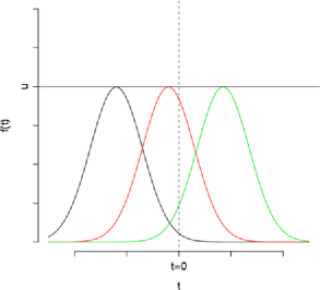
Figure 1: One-dimensional example.

Second, as mentioned before, the conditional distributions of $f(t)$ are different given $\{I_{\sigma}(T)>b\}$ or $\{\sup_{T}f(t)>u\}$. This is why the two constants in Theorem 1 ($H$) and Proposition 1 ($G$) are different. The difference is due to the fact that the symmetric difference between $\{\sup_{T}f(t)>u\}$ and $\{\int_{T}e^{f(t)}\,dt>b\}$ is substantial though their overlap is significant too. Consider the following situation that contributes to the difference. $\sup_{T}f(t)$ is slightly less than $u$ [e.g., by a magnitude of $O(u^{-1})$]. For this case, $I_{\sigma}(T)$ still has a large chance to be greater than $b$. For this sake we will need to consider the contribution of $\Delta f(0)$. As is shown in the technical proof, if $t^{*}=\arg\sup f(t)=0$ and $\partial f(0)=0$, then a sufficient and necessary condition for $I_{\sigma}(T)>b$ is that

$$f(0)+\frac{1}{2\sigma}\operatorname{Tr}\bigl{(}u^{-1}\Delta f(0)+I\bigr{)}>u+o(u^{-1}),$$

where $\mathrm{Tr}$ denotes the trace of a squared matrix. Note that conditional on $f(0)=u$, $E(\Delta f(0)|f(0)=u)=-uI$. Therefore, $\Delta f(0)+uI$ is of size $O(1)$. One well-known result is that the trace of a symmetric matrix is the sum of its eigenvalues. Let $\lambda_{i}$ be the eigenvalues of $u^{-1}\Delta f(0)+I=\mathbf{z}/u$. Then, the sufficient and necessary condition is translated to $f(0)+\frac{1}{2\sigma}\sum_{i=1}^{d}\lambda_{i}>u$. This also suggests that, conditional on $I_{\sigma}(T)>b$, $w=f(0)-u$ is of size $O(u^{-1})$. This forms the intuition behind the proof of Theorem 2.

The proof of Theorem 1 consists of two steps presented in Sections 3.1 and 3.2, respectively. Each of the two steps is summarized as one theorem.

3.1 Step 1

Construct a cover of $T$, $\{A_{1},\ldots,A_{n}\}$, such that $T\subset\bigcup_{i=1}^{n}A_{i}$. Each $A_{i}$ is a closed square, $\operatorname{mes}(A_{i}\cap A_{j})=0$ for $i\neq j$. Because $T$ is Jordan measurable, as $\sup_{i}\operatorname{mes}(A_{i})\rightarrow 0$, $\operatorname{mes}(\bigcup_{i=1}^{n}A_{i})-\operatorname{mes}(T)\rightarrow 0$. To simplify the analysis, we make each $A_{i}$ of identical shape and let $A_{i}=\{t_{i}+s\dvtx\allowbreak s\in[0,a_{b}]^{d}\}$. The size of the partition $n$ and choice of $a_{b}$ depend on the threshold $b$. The first step analysis involves computing the integral $p_{i}\triangleq P(\int_{A_{i}}e^{\sigma f(t)}\,dt>b)$. Because $f$ is homogeneous, it is sufficient to study $p_{1}$.

The basic strategy to approximate $p_{1}$ is as follows. Because $f$ is at least three times differentiable, the first and second derivatives are almost surely well defined. Without loss of generality, we assume that $0\in A_{1}$. Conditional on $(f(0),\partial f(0),\Delta f(0))$, $f(t)=f(0)+\partial f(0)^{\top}t+\frac{1}{2}t^{\top}\Delta f(0)t+g_{3}(t)+g_{4}(t)+R(t)+g(t)$, where $g(t)$ is a Gaussian field with mean zero and variance of order $O(|t|^{6})$. Then,

$$\qquad p_{1} = P\biggl{(}\int_{A_{1}}e^{\sigma f(t)}\,dt>b\biggr{)}$$

$$= \int h(w,y,z)$$

$$\hphantom{\int}{}\times P\biggl{(}\int_{A_{1}}e^{\sigma[u-w+y^{\top}t+(1/2)t^{\top}(-uI+\mathbf{z})t+g_{3}(t)+g_{4}(t)+R(t)+g(t)]}\,dt$$

$$\hphantom{\int{}\times P\biggl{(}}{}>b\biggr{)}\,dw\,dy\,dz,$$

where $h(w,y,z)$ is the density function of $(f(0),\partial f(0),\Delta f(0))$ evaluated at $(u-w,y,u\mu_{20}+z)$, which is a multivariate Gaussian random vector. Let $u$ be defined in (8). There exists a $\delta>0$ (small enough) such that if we let $A_{i}$’s be squares of size $\varepsilon=O(1)u^{-1/2+\delta}$ and, hence, $n=O(1)\operatorname{mes}(T)u^{d/2-d\delta}$, the asymptotics of $p_{i}$ can be derived by repeatedly using Taylor’s expansion and evaluating the integral on the right-hand side of (3.1). The main result of this step is presented as follows. It establishes a similar result to that of Theorem 1 but within a much smaller domain.

Theorem 2

Let $f$ be a Gaussian random field living in $T$ satisfying conditions (C1)–(C4). Let $A_{1}=\Xi_{\varepsilon}=\{t\dvtx|t|_{\infty}<\varepsilon\}$, where $|t|_{\infty}={\max_{i}}|t_{i}|$. Let $u$ and $H$ be defined in Theorem 1. Without loss of generality, assume $\Xi_{\varepsilon}\subset T$ with $\varepsilon=\kappa u^{\delta-1/2}$ for some $\delta$ small enough and $u$ large enough. Then, for any $\kappa>0$

$$p_{1}=p(\Xi_{\varepsilon})=P\biggl{(}\int_{\Xi_{\varepsilon}}e^{\sigma f(t)}\,dt>b\biggr{)}=\bigl{(}1+o(1)\bigr{)}H\operatorname{mes}(\Xi_{\varepsilon})u^{d-1}e^{-u^{2}/2}$$

as $b\rightarrow\infty$.

The proof of this theorem is in Section 4. We will then choose each $A_{i}$ to be of the same shape as $\Xi_{\varepsilon}$. Then, all the $p_{i}$’s are identical.

3.2 Step 2

The second step is to show that with the particular choice of $A_{i}$ in the first step, $P(\int_{T}e^{\sigma f(t)}\,dt>b)=(1+o(1))\sum_{i=1}^{n}p_{i}$. We first present the main result of the second step.

Theorem 3

Let $f$ be a Gaussian random field satisfying conditions (C1)–(C4) and $\varepsilon$ be chosen in Theorem 2. Let $\mathbf{k}\in\mathbb{Z}^{d}$ and $\Xi_{\varepsilon,\mathbf{k}}=2\mathbf{k}\varepsilon+\Xi_{\varepsilon}$. Further, let $\mathcal{C}^{-}=\{\mathbf{k}\dvtx\Xi_{\varepsilon,\mathbf{k}}\subset T\}$ and $\mathcal{C}^{+}=\{\mathbf{k}\dvtx\Xi_{\varepsilon,\mathbf{k}}\cap T\neq\varnothing\}$, then

$$P\biggl{(}I_{\sigma}\biggl{(}\bigcup_{\mathbf{k}\in\mathcal{C}^{+}}\Xi_{\varepsilon,\mathbf{k}}\biggr{)}>b\biggr{)}=\bigl{(}1+o(1)\bigr{)}\sum_{\mathbf{k}\in\mathcal{C}^{+}}P\bigl{(}I_{\sigma}(\Xi_{\varepsilon,\mathbf{k}})>b\bigr{)}$$

and

$$P\biggl{(}I_{\sigma}\biggl{(}\bigcup_{\mathbf{k}\in\mathcal{C}^{-}}\Xi_{\varepsilon,\mathbf{k}}\biggr{)}>b\biggr{)}=\bigl{(}1+o(1)\bigr{)}\sum_{\mathbf{k}\in\mathcal{C}^{-}}P\bigl{(}I_{\sigma}(\Xi_{\varepsilon,\mathbf{k}})>b\bigr{)}.$$

We consider

$$I_{\sigma}\biggl{(}\bigcup_{\mathbf{k}\in\mathcal{C}^{+}}\Xi_{\varepsilon,\mathbf{k}}\biggr{)}=\sum_{\mathbf{k}\in\mathcal{C}^{+}}I_{\sigma}(\Xi_{\varepsilon,\mathbf{k}})$$

as a sum of finitely many dependently and identically distributed random variables. The conclusion of the above theorem implies that the tail distribution of the sum of these dependent variables exhibits the so-called “one big jump” feature—the high excursion of the sum is mainly caused by just one component being large. This result is similar to that of the sum of correlated log-normal r.v.’s. Nevertheless, the gap between the analyses of finite sum and integral is substantial because the correlation between fields in adjacent squares tends to $1$. For finite sums, the correlation is always bounded away from $1$. The key step in the proof of Theorem 3 is that the $\varepsilon$ defined in Theorem 2, though tends to zero as $b\rightarrow\infty$, is large enough such that the one-big-jump principle still applies. We will connect the event of high excursion of $I_{\sigma}(\bigcup_{\mathbf{k}\in\mathcal{C}^{+}}\Xi_{\varepsilon,\mathbf{k}})$ to the high excursion of $\sup_{\bigcup_{\mathbf{k}\in\mathcal{C}^{+}}\Xi_{\varepsilon,\mathbf{k}}}f(t)$ and apply existing results on the bound on the supremum of Gaussian random fields. A short list of recent related literature on the “one-big-jump” principle and multivariate Gaussian random variables is FA09 , DDS08 , AR08 .

With the preparation of the two steps, we are ready to present the proof for Theorem 1. Proof of Theorem 1 From Theorem 2,

$$\sum_{\mathbf{k}\in\mathcal{C}^{+}}P\bigl{(}I_{\sigma}(\Xi_{\varepsilon,\mathbf{k}})>b\bigr{)} = \bigl{(}1+o(1)\bigr{)}H\operatorname{mes}\biggl{(}\bigcup_{\mathbf{k}\in\mathcal{C}^{+}}\Xi_{\varepsilon,\mathbf{k}}\biggr{)}u^{d-1}e^{-u^{2}/2},$$

$$\sum_{\mathbf{k}\in\mathcal{C}^{-}}P\bigl{(}I_{\sigma}(\Xi_{\varepsilon,\mathbf{k}})>b\bigr{)} = \bigl{(}1+o(1)\bigr{)}H\operatorname{mes}\biggl{(}\bigcup_{\mathbf{k}\in\mathcal{C}^{-}}\Xi_{\varepsilon,\mathbf{k}}\biggr{)}u^{d-1}e^{-u^{2}/2}.$$

Therefore, thanks to Theorem 3,

$$P\bigl{(}I_{\sigma}(T)>b\bigr{)} \geq P\biggl{(}I_{\sigma}\biggl{(}\bigcup_{\mathbf{k}\in\mathcal{C}^{-}}\Xi_{\varepsilon,\mathbf{k}}\biggr{)}>b\biggr{)}$$

$$\geq \bigl{(}1+o(1)\bigr{)}H\operatorname{mes}\biggl{(}\bigcup_{\mathbf{k}\in\mathcal{C}^{-}}\Xi_{\varepsilon,\mathbf{k}}\biggr{)}u^{d-1}e^{-u^{2}/2};$$

similarly,

$$P\bigl{(}I_{\sigma}(T)>b\bigr{)} \leq P\biggl{(}I_{\sigma}\biggl{(}\bigcup_{\mathbf{k}\in\mathcal{C}^{+}}\Xi_{\varepsilon,\mathbf{k}}\biggr{)}>b\biggr{)}$$

$$\leq \bigl{(}1+o(1)\bigr{)}H\operatorname{mes}\biggl{(}\bigcup_{\mathbf{k}\in\mathcal{C}^{+}}\Xi_{\varepsilon,\mathbf{k}}\biggr{)}u^{d-1}e^{-u^{2}/2}.$$

Jordan measurability of $T$ implies that

$$\operatorname{mes}\biggl{(}\bigcup_{\mathbf{k}\in\mathcal{C}^{+}}\Xi_{\varepsilon,\mathbf{k}}\biggr{)}-\operatorname{mes}\biggl{(}\bigcup_{\mathbf{k}\in\mathcal{C}^{-}}\Xi_{\varepsilon,\mathbf{k}}\biggr{)}\rightarrow 0{+}.$$

Therefore,

$$P\bigl{(}I_{\sigma}(T)>b\bigr{)}=\bigl{(}1+o(1)\bigr{)}H\operatorname{mes}(T)u^{d-1}e^{-u^{2}/2}.$$

4 Proof for Theorem 2

In this section we present the proof of Theorem 2. We arrange all the lemmas and their proofs in the Appendix. Proof of Theorem 2 We evaluate the probability by conditioning on $(f(0),\partial f(0),\partial^{2}f(0))$,

$$p(\Xi_{\varepsilon}) = P\biggl{(}\int_{\Xi_{\varepsilon}}e^{\sigma f(t)}\,dt>b\biggr{)}$$

$$= \int_{\mathcal{R}}h(w,y,z)$$

$$\hskip 11.0pt{}\times P\biggl{(}\int_{\Xi_{\varepsilon}}e^{\sigma f(t)}\,dt>b\Big{|}f(0)=u-w,\partial f(0)=y,$$

$$\hskip 146.6pt\partial^{2}f(0)=u\mu_{02}+z\biggr{)}\,dw\,dy\,dz$$

$$= \int_{\mathcal{R}}h(w,y,z)P\biggl{(}\int_{\Xi_{\varepsilon}}e^{\sigma E(t)+\sigma g(t)}\,dt>b\biggr{)}\,dw\,dy\,dz,$$

where $\mathcal{R}=R^{(d+1)(d+2)/2}$ and $h(w,y,z)$ is the density function of $(f(0),\partial f(0)$, $\partial^{2}f(0))$ evaluated at $(u-w,y,u\mu_{02}+z)$. Now we take a closer look at the integrand inside the above integral. Conditional on $f(0)=u-w,\partial f(0)=y$, $\partial^{2}f(0)=u\mu_{02}+z$,

$$I_{\sigma}(\Xi_{\varepsilon}) = \int_{|t|_{\infty}<\varepsilon}e^{\sigma E(t)+\sigma g(t)}\,dt$$

$$= \int_{|t|_{\infty}<\varepsilon}\exp\biggl{\{}\sigma\biggl{[}u-w+y^{\top}t+\frac{1}{2}t^{\top}(-uI+\mathbf{z})t$$

$$\hphantom{\int_{|t|_{\infty}<\varepsilon}\exp\biggl{\{}}\hskip 17.0pt{}+g_{3}(t)+g_{4}(t)+R(t)+g(t)\biggr{]}\biggr{\}}\,dt$$

$$= \det(uI-\mathbf{z})^{-1/2}$$

$${}\times\int_{|(uI-\mathbf{z})^{-1/2}t|_{\infty}<\varepsilon}e^{\sigma\{u-w+({1/2})y^{\top}(uI-\mathbf{z})^{-1}y\}}$$

$${}\times\exp\biggl{\{}\sigma\biggl{[}-\frac{1}{2}\bigl{(}t-(uI-\mathbf{z})^{-1/2}y\bigr{)}^{\top}\bigl{(}t-(uI-\mathbf{z})^{-1/2}y\bigr{)}$$

$$\hskip 45.2pt{}+g_{3}\bigl{(}(uI-\mathbf{z})^{-1/2}t\bigr{)}+g_{4}\bigl{(}(uI-\mathbf{z})^{-1/2}t\bigr{)}$$

$$\hskip 69.6pt{}+R\bigl{(}(uI-\mathbf{z})^{-1/2}t\bigr{)}+g\bigl{(}(uI-\mathbf{z})^{-1/2}t\bigr{)}\biggr{]}\biggr{\}}\,dt.$$

For the second equality, we plugged in (5). For the last step, we first change the variable from $t$ to $(uI-\mathbf{z})^{1/2}t$ and then write the exponent in a quadratic form of $t$. We write the term inside the exponent without the factor $\sigma$ as

$$\qquad J(t) = -\tfrac{1}{2}\bigl{(}t-(uI-\mathbf{z})^{-1/2}y\bigr{)}^{\top}\bigl{(}t-(uI-\mathbf{z})^{-1/2}y\bigr{)}+g_{3}\bigl{(}(uI-\mathbf{z})^{-1/2}t\bigr{)}$$

$${}+g_{4}\bigl{(}(uI-\mathbf{z})^{-1/2}t\bigr{)}+R\bigl{(}(uI-\mathbf{z})^{-1/2}t\bigr{)},$$

which is asymptotically a quadratic form. But, as is shown later, $g_{3}$ and $g_{4}$ terms do play a role in the calculation. Also, it is useful to keep in mind that $J(t)$ depends on $y$ and $z$. Hence, we can write

$$I_{\sigma}(\Xi_{\varepsilon}) = \int_{|t|_{\infty}<\varepsilon}e^{\sigma f(t)}\,dt$$

$$= \det(uI-\mathbf{z})^{-1/2}e^{\sigma\{u-w+({1/2})y^{\top}(uI-\mathbf{z})^{-1}y\}}$$

$${}\times\int_{|(uI-\mathbf{z})^{-1/2}t|_{\infty}<\varepsilon}e^{\sigma J(t)+\sigma g((uI-\mathbf{z})^{-1/2}t)}\,dt.$$

Let

$$e^{H_{0}}=\int_{R^{d}}e^{-({\sigma/2})t^{\top}t}\,dt=(2\pi/\sigma)^{d/2}.$$ (14)

Let $u$ solve

$$u^{-d/2}e^{\sigma u+H_{0}}=b.$$ (15)

Then,

$$\int_{\Xi_{\varepsilon}}e^{\sigma f(t)}\,dt>b,$$

if and only if

$$\det(uI-{\mathbf{z}})^{-1/2}e^{\sigma\{u-w+({1/2})y^{\top}(uI-{\mathbf{z}})^{-1}y\}}\int_{|(uI-{\mathbf{z}})^{-1/2}t|_{\infty}<\varepsilon}e^{\sigma J(t)+\sigma g((uI-{\mathbf{z}})^{-1/2}t)}\,dt$$

$$\qquad>u^{-d/2}e^{\sigma u+H_{0}}.$$

We take the logarithm on both sides and rewrite the above inequality and have

$$0 < \frac{\sigma}{2}y^{\top}(uI-\mathbf{z})^{-1}y-\sigma w-\frac{1}{2}\log\det(I-u^{-1}\mathbf{z})$$

$${}+\log\int_{|(uI-\mathbf{z})^{-1/2}t|_{\infty}<\varepsilon}e^{\sigma J(t)}\,dt-H_{0}$$

$${}+\log E\exp\bigl{(}\sigma g\bigl{(}(uI-\mathbf{z})^{-1/2}S\bigr{)}\bigr{)}$$

$$= A(w,y,z)+\log E\exp\bigl{(}\sigma g\bigl{(}(uI-\mathbf{z})^{-1/2}S\bigr{)}\bigr{)},$$ (17)

where $S$ is a random variable on the region that $|(uI-\mathbf{z})^{-1/2}S|_{\infty}\leq\varepsilon$ with density proportional to $e^{\sigma J(s)}$ and

$$A(w,y,z) = \frac{\sigma}{2}y^{\top}(uI-\mathbf{z})^{-1}y-\sigma w-\frac{1}{2}\log\det(I-u^{-1}\mathbf{z})$$

$${}+\log\int_{|(uI-\mathbf{z})^{-1/2}t|<\varepsilon}e^{\sigma J(t)}\,dt-H_{0}.$$

Thanks to Lemma 1, we only need to consider the set that

$$\mathcal{L} = \{|f(0)-u|\leq u^{2\delta+\varepsilon_{0}},$$

$$\hphantom{\{}|\partial f(0)|\leq u^{{1}/{2}+\delta+\varepsilon_{0}},|\partial^{2}f(0)-u\mu_{20}|\leq u^{{1/2}+\varepsilon_{0}}\}.$$

Also, by abusing notation, we write

$$\mathcal{L}=\{|w|\leq u^{2\delta+\varepsilon_{0}},|y|\leq u^{{1}/{2}+\delta+\varepsilon_{0}},|z|\leq u^{{1}/{2}+\varepsilon_{0}}\}.$$ (20)

Lemma 2 gives the form of $h(w,y,z)$. We plug in the results in Lemmas 1 and 2,

$$p(\Xi_{\varepsilon}) = \int_{\mathcal{R}}h(w,y,z)$$

$$\hphantom{\int_{\mathcal{R}}}{}\times P\bigl{(}A(w,y,z)+\log E\exp\bigl{(}\sigma g\bigl{(}(uI-\mathbf{z})^{-1/2}S\bigr{)}\bigr{)}>0\bigr{)}\,dw\,dy\,dz$$

$$= o(1)u^{-\alpha}e^{-u^{2}/2}$$

$${}+\int_{\mathcal{L}}h(w,y,z)$$

$$\hphantom{{}+\int_{\mathcal{L}}}{}\times P\bigl{(}A(w,y,z)+\log E\exp\bigl{(}\sigma g\bigl{(}(uI-\mathbf{z})^{-1/2}S\bigr{)}\bigr{)}>0\bigr{)}\,dw\,dy\,dz$$

$$= o(1)u^{-\alpha}e^{-u^{2}/2}$$

$${}+\frac{1}{(2\pi)^{(d+1)(d+2)/4}}|\Gamma|^{-1/2}$$

$$\hskip 11.0pt{}\times\int_{\mathcal{L}}P\bigl{(}A(w,y,z)+\log E\exp\bigl{(}\sigma g\bigl{(}(uI-\mathbf{z})^{-1/2}S\bigr{)}\bigr{)}>0\bigr{)}$$

$$\hskip 34.2pt{}\times\exp\biggl{\{}-\biggl{[}\frac{1}{2}u^{2}+\frac{u}{\sigma}A(w,y,z)$$

$$\hskip 81.3pt{}+\frac{1}{2}y^{\top}\bigl{(}I-(I-{\mathbf{z}}/u)^{-1}\bigr{)}y$$

$$\hskip 81.3pt{}+\frac{1}{2}\frac{(w+\mu_{20}\mu_{22}^{-1}z)^{2}}{1-\mu_{20}\mu_{22}^{-1}\mu_{02}}+\frac{1}{2}z^{\top}\mu_{22}^{-1}z$$

$$\hskip 81.3pt{}+\frac{u}{2\sigma}\log\det(I-u^{-1}\mathbf{z})$$

$$\hskip 81.3pt{}-\frac{u}{\sigma}\log\int_{|(uI-\mathbf{z})^{-1/2}t|<\varepsilon}e^{\sigma J(t)}\,dt+\frac{u}{\sigma}H_{0}\biggr{]}\biggr{\}}\,dw\,dy\,dz.$$

We define

$$\mathcal{I} = \frac{1}{2}u^{2}+\frac{u}{\sigma}A(w,y,z)+\frac{1}{2}y^{\top}\bigl{(}I-(I-\mathbf{z}/u)^{-1}\bigr{)}y$$

$${}+\frac{1}{2}\frac{(w+\mu_{20}\mu_{22}^{-1}z)^{2}}{1-\mu_{20}\mu_{22}^{-1}\mu_{02}}+\frac{1}{2}z^{\top}\mu_{22}^{-1}z+\frac{u}{2\sigma}\log\det(I-u^{-1}\mathbf{z})$$

$${}-\frac{u}{\sigma}\log\int_{|(uI-\mathbf{z})^{-1/2}t|<\varepsilon}e^{\sigma J(t)}\,dt+\frac{u}{\sigma}H_{0},$$

and proceed with some tedious algebra to write $\mathcal{I}$ in a friendly form for integration. First notice that

$$(I-u^{-1}\mathbf{z})^{-1}=\sum_{k=0}^{\infty}u^{-n}\mathbf{z}^{n}.$$

Plug this into the third term of $\mathcal{I}$ and obtain

$$\mathcal{I} = \frac{1}{2}u^{2}+\frac{u}{\sigma}A(w,y,z)-\bigl{(}1+O(|z|/u)\bigr{)}\frac{u^{-1}}{2}y^{\top}\mathbf{z}y$$

$${}+\frac{1}{2}\frac{(w+\mu_{20}\mu_{22}^{-1}z)^{2}}{1-\mu_{20}\mu_{22}^{-1}\mu_{02}}+\frac{1}{2}z^{\top}\mu_{22}^{-1}z+\frac{u}{2\sigma}\log\det(I-u^{-1}{\mathbf{z}})$$

$${}-\frac{u}{\sigma}\log\int_{|(uI-\mathbf{z})^{-1/2}t|<\varepsilon}e^{\sigma J(t)}\,dt+\frac{u}{\sigma}H_{0}.$$

Situation 1 of Lemma 5

Adopt the notation in Lemmas 4 and 5. Note that according to the definition of $Y$ in Lemma 4 that

$$Y = (y_{i}^{2},i=1,\ldots,d,2y_{i}y_{j},1\leq i<j\leq d)^{\top},$$

$$\mathbf{1} = (\underbrace{1,\ldots,1}_{d},\underbrace{0,\ldots,0}_{d(d-1)/2})^{\top},$$

we obtain that

$$y^{\top}\mathbf{z}y=Y^{\top}z.$$

We plug in results of Lemmas 4 and 5. First, considering the first situation in Lemma 5, that is, $\mathcal{L}_{1}=\mathcal{L}\cap\{|(uI-\mathbf{z})^{-1/2}y|_{\infty}\leq\kappa u^{\delta}-u^{\delta/2}\}$, we have

$$\mathcal{I} = \frac{1}{2}u^{2}+\frac{u}{\sigma}A(w,y,z)-\bigl{(}1+O(|z|/u)\bigr{)}\frac{u^{-1}}{2}Y^{\top}z$$

$${}+\frac{1}{2}\frac{(w+\mu_{20}\mu_{22}^{-1}z)^{2}}{1-\mu_{20}\mu_{22}^{-1}\mu_{02}}+\frac{1}{2}z^{\top}\mu_{22}^{-1}z+\frac{u}{2\sigma}\log\det(I-u^{-1}\mathbf{z})$$

$${}+\frac{1}{8}(u^{-1}Y+\mathbf{1}/\sigma)^{\top}\mu_{22}(u^{-1}Y+\mathbf{1}/\sigma)-\frac{1}{8\sigma^{2}}\mathbf{1}^{\top}\mu_{22}\mathbf{1}$$

$${}+\frac{u}{\sigma}H_{0}-\frac{u}{\sigma}H\bigl{(}(uI-\mathbf{z})^{-1/2}y,(uI-\mathbf{z})^{1/2},\varepsilon\bigr{)}$$

$${}-\frac{1}{8\sigma^{2}}\sum_{i}\partial_{iiii}C(0)+o(1).$$

Also, it is useful to keep in mind that $\mathbf{1}$ is NOT a vector of $1$’s. The next step is to plug in the result of Lemma 3 and replace the $\log\det(I-u^{-1}\mathbf{z})$ term by

$$-u^{-1}\operatorname{Tr}(\mathbf{z})+\tfrac 12u^{-2}\mathcal{E}^{2}(\mathbf{z})+o(u^{-1})$$

$$\qquad=-u^{-1}\mathbf{1}^{\top}z+\tfrac 12u^{-2}\mathcal{E}^{2}(\mathbf{z})+o(u^{-1})$$

and obtain

$$\mathcal{I} = \frac{1}{2}u^{2}+\frac{u}{\sigma}A(w,y,z)-\bigl{(}1+O(|z|/u)\bigr{)}\frac{u^{-1}}{2}Y^{\top}z$$

$${}+\frac{1}{2}\frac{(w+\mu_{20}\mu_{22}^{-1}z)^{2}}{1-\mu_{20}\mu_{22}^{-1}\mu_{02}}+\frac{1}{2}z^{\top}\mu_{22}^{-1}z-\frac{1}{2\sigma}\mathbf{1}^{\top}z+\frac{1}{4\sigma u}\mathcal{E}^{2}(\mathbf{z})$$

$${}+\frac{1}{8}(u^{-1}Y+\mathbf{1}/\sigma)^{\top}\mu_{22}(u^{-1}Y+\mathbf{1}/\sigma)-\frac{1}{8\sigma^{2}}\mathbf{1}^{\top}\mu_{22}\mathbf{1}$$

$${}+\frac{u}{\sigma}H_{0}-\frac{u}{\sigma}H\bigl{(}(uI-\mathbf{z})^{-1/2}y,(uI-\mathbf{z})^{1/2},\varepsilon\bigr{)}$$

$${}-\frac{1}{8\sigma^{2}}\sum_{i}\partial_{iiii}C(0)+o(1).$$

Then, we group the terms $-(1+O(|z|/u))\frac{u^{-1}}{2}Y^{\top}z$ and $-\frac{1}{2\sigma}\mathbf{1}^{\top}z$ and leave the $O(|z|/u)$ to the end and have

$$\mathcal{I} = \frac{1}{2}u^{2}+\frac{u}{\sigma}A(w,y,z)+\frac{1}{2}\frac{(w+\mu_{20}\mu_{22}^{-1}z)^{2}}{1-\mu_{20}\mu_{22}^{-1}\mu_{02}}$$

$${}+\frac{1}{2}z^{\top}\mu_{22}^{-1}z-\frac{1}{2}(u^{-1}Y+\mathbf{1}/\sigma)^{\top}z$$

$${}+\frac{1}{8}(u^{-1}Y+\mathbf{1}/\sigma)^{\top}\mu_{22}(u^{-1}Y+\mathbf{1}/\sigma)$$

$${}+\frac{u}{\sigma}H_{0}-\frac{u}{\sigma}H\bigl{(}(uI-\mathbf{z})^{-1/2}y,(uI-\mathbf{z})^{1/2},\varepsilon\bigr{)}$$

$${}-\frac{1}{8\sigma^{2}}\mathbf{1}^{\top}\mu_{22}\mathbf{1}-\frac{1}{8\sigma^{2}}\sum_{i}\partial_{iiii}C(0)+o(1)$$

$${}+O(u^{-2}|z|^{2}|y|^{2})+O(u^{-1}\mathcal{E}^{2}(\mathbf{z})).$$

Note that second and third lines in the above display is in fact in a quadratic form. We then have

$$\mathcal{I} = \frac{1}{2}u^{2}+\frac{u}{\sigma}A(w,y,z)+\frac{1}{2}\frac{(w+\mu_{20}\mu_{22}^{-1}z)^{2}}{1-\mu_{20}\mu_{22}^{-1}\mu_{02}}$$

$${}+\frac{1}{2}\biggl{[}\mu_{22}^{-1/2}z-\frac{1}{2}\mu_{22}^{1/2}(u^{-1}Y+\mathbf{1}/\sigma)\biggr{]}^{\top}$$

$$\hskip 11.0pt{}\times\biggl{[}\mu_{22}^{-1/2}z-\frac{1}{2}\mu_{22}^{1/2}(u^{-1}Y+\mathbf{1}/\sigma)\biggr{]}$$

$${}+\frac{u}{\sigma}H_{0}-\frac{u}{\sigma}H\bigl{(}(uI-\mathbf{z})^{-1/2}y,(uI-\mathbf{z})^{1/2},\varepsilon\bigr{)}$$

$${}-\frac{1}{8\sigma^{2}}\mathbf{1}^{\top}\mu_{22}\mathbf{1}-\frac{1}{8\sigma^{2}}\sum_{i}\partial_{iiii}C(0)+o(1)$$

$${}+O(u^{-2}|z|^{2}|y|^{2})+O(u^{-1}\mathcal{E}^{2}(\mathbf{z})).$$

Now, consider another change of variable,

$$A = A(w,y,z),$$

$$B = \mu_{22}^{-1/2}z-\tfrac{1}{2}\mu_{22}^{1/2}(u^{-1}Y+\mathbf{1}/\sigma),\qquad y=y.$$

Then, by noting that $\mu_{20}$ is a row vector in which the first $d$ entries are $-1$’s and the rest are $0$’s, we have

$$w+\mu_{20}\mu_{22}^{-1}z=-\frac{A}{\sigma}+\mu_{20}\mu_{22}^{-{1/2}}B+\frac{1}{2\sigma}\mu_{20}\mathbf{1}+o(1).$$

Therefore, we have

$$\mathcal{I} = \frac{1}{2}u^{2}+\frac{u}{\sigma}A+\frac{1}{2}B^{\top}B$$

$${}+\frac{1}{2}\frac{(-{A}/{\sigma}+\mu_{20}\mu_{22}^{-{1/2}}B+({1}/({2\sigma}))\mu_{20}\mathbf{1}+o(1))^{2}}{1-\mu_{20}\mu_{22}^{-1}\mu_{02}}$$

$${}+\frac{u}{\sigma}H_{0}-\frac{u}{\sigma}H\bigl{(}(uI-\mathbf{z})^{-1/2}y,(uI-\mathbf{z})^{1/2},\varepsilon\bigr{)}$$

$${}-\frac{1}{8\sigma^{2}}\mathbf{1}^{\top}\mu_{22}\mathbf{1}-\frac{1}{8\sigma^{2}}\sum_{i}\partial_{iiii}C(0)+o(1)+O(u^{-2}|z|^{2}|y|^{2})+O(u^{-1}\mathcal{E}^{2}({\mathbf{z}})).$$

We write $X_{u}=o_{p}(1)$ if $X_{u}\rightarrow 0$ in probability as $u\rightarrow\infty$. We insert the above form back to the integral in (4) and apply Lemma 7,

$$p(\Xi_{\varepsilon}) = o(1)u^{-\alpha}e^{-u^{2}/2}$$

$${}+\frac{1}{(2\pi)^{(d+1)(d+2)/4}}|\Gamma|^{-1/2}$$

$$\hskip 10.0pt{}\times\int_{\mathcal{L}}P\bigl{(}u\cdot A>o_{p}(1)\bigr{)}$$

$$\hskip 34.3pt{}\times\exp\biggl{\{}-\biggl{[}\frac{1}{2}u^{2}+\frac{u}{\sigma}A+\frac{1}{2}B^{\top}B$$

$$\hskip 81.7pt{}+\frac{1}{2}\frac{(-{A}/{\sigma}+\mu_{20}\mu_{22}^{-{1/2}}B+{1}/({2\sigma})\mu_{20}\mathbf{1}+o(1))^{2}}{1-\mu_{20}\mu_{22}^{-1}\mu_{02}}$$

$$\hskip 81.7pt{}+\frac{u}{\sigma}H_{0}-\frac{u}{\sigma}H\bigl{(}(uI-\mathbf{z})^{-1/2}y,(uI-\mathbf{z})^{1/2},\varepsilon\bigr{)}$$

$$\hskip 81.7pt{}-\frac{1}{8\sigma^{2}}\mathbf{1}^{\top}\mu_{22}\mathbf{1}-\frac{1}{8\sigma^{2}}\sum_{i}\partial_{iiii}C(0)+o(1)$$

$$\hskip 81.7pt\hskip 51.4pt{}+O(u^{-2}|z|^{2}|y|^{2})+O(u^{-1}\mathcal{E}^{2}({\mathbf{z}}))\biggr{]}\biggr{\}}\,dw\,dy\,dz.$$

Note that Jacobian determinant is

$$\biggl{|}\det\biggl{(}\frac{\partial(w,z,y)}{\partial(A,B,y)}\biggr{)}\biggr{|}=\sigma^{-1}\det(\mu_{22})^{1/2}.$$

Note that when $|(uI-{\mathbf{z}})^{-1/2}y|\leq\kappa u^{\delta}-u^{\delta/2}$ (the first situation in Lemma 5),

$$uH_{0}-uH\bigl{(}(uI-\mathbf{z})^{-1/2}y,(uI-\mathbf{z})^{1/2},\varepsilon\bigr{)}=o(1).$$

Then, with another change of variable, $A^{\prime}=uA$, the integration on $\mathcal{L}_{1}$ is

$$\int_{\mathcal{L}_{1}}h(w,y,z)P\biggl{(}\int_{\Xi_{\varepsilon}}e^{\sigma E(t)+\sigma g(t)}\,dt>b\biggr{)}\,dw\,dy\,dz$$

$$\qquad=\frac{|\Gamma|^{-1/2}}{(2\pi)^{(d+1)(d+2)/4}}$$

$$\qquad\quad{}\times\int_{\mathcal{L}_{1}}P\bigl{(}u\cdot A>o_{p}(1)\bigr{)}$$

$$\qquad\quad{}\times\exp\biggl{\{}-\biggl{[}\frac{1}{2}u^{2}+\frac{u}{\sigma}A+\frac{1}{2}B^{\top}B$$

$$\qquad\quad\hskip 74.88pt{}+\frac{1}{2}\frac{(-{A}/{\sigma}+\mu_{20}\mu_{22}^{-{1/2}}B+{1}/({2\sigma})\mu_{20}\mathbf{1}+o(1))^{2}}{{1-\mu_{20}\mu_{22}^{-1}\mu_{02}}}$$ (24)

$$\qquad\quad\hskip 73.8pt{}+\frac{u}{\sigma}H_{0}-\frac{u}{\sigma}H\bigl{(}(uI-\mathbf{z})^{-1/2}y,(uI-\mathbf{z})^{1/2},\varepsilon\bigr{)}$$

$$\qquad\quad\hskip 73.8pt{}-\frac{1}{8\sigma^{2}}\mathbf{1}^{\top}\mu_{22}\mathbf{1}-\frac{1}{8\sigma^{2}}\sum_{i}\partial_{iiii}C(0)+o(1)$$

$$\qquad\quad\hskip 130.6pt{}+o(u^{-2}|z|^{2}|y|^{2})+O(u^{-1}\mathcal{E}^{2}({\mathbf{z}}))\biggr{]}\biggr{\}}\,dw\,dy\,dz$$

$$\qquad=\frac{\sigma^{-1}|\Gamma|^{-1/2}}{(2\pi)^{(d+1)(d+2)/4}}\det(\mu_{22})^{1/2}$$

$$\qquad\quad{}\times e^{-({1/2})u^{2}+({1}/({8\sigma^{2}}))\mathbf{1}^{\top}\mu_{22}\mathbf{1}+({1}/({8\sigma^{2}}))\sum_{i}\partial_{iiii}C(0)}$$

$$\qquad\quad{}\times\int_{\mathcal{L}_{1}}P\bigl{(}u\cdot A>o_{p}(1)\bigr{)}$$

$$\qquad\quad{}\times\exp\biggl{\{}-\biggl{[}\frac{u}{\sigma}\cdot A+\frac{B^{\top}B}{2}$$

$$\qquad\quad\hskip 46.7pt{}+\frac{(-{A}/{\sigma}+\mu_{20}\mu_{22}^{-{1/2}}B+{1}/({2\sigma})\mu_{20}\mathbf{1}+o(1))^{2}}{2(1-\mu_{20}\mu_{22}^{-1}\mu_{02})}$$

$$\qquad\quad\hskip 46.7pt\hskip 30.5pt{}+o(1)+O\bigl{(}u^{-2}|z|^{2}|y|^{2}+u^{-1}\mathcal{E}^{2}({\mathbf{z}})\bigr{)}\biggr{]}\biggr{\}}\,dA\,dB\,dy$$

$$\qquad=\frac{\sigma^{-1}|\Gamma|^{-1/2}}{(2\pi)^{(d+1)(d+2)/4}}\det(\mu_{22})^{1/2}u^{-1}$$

$$\qquad\quad{}\times e^{-({1/2})u^{2}+({1}/({8\sigma^{2}}))\mathbf{1}^{\top}\mu_{22}\mathbf{1}+({1}/({8\sigma^{2}}))\sum_{i}\partial_{iiii}C(0)}$$

$$\qquad\quad{}\times\int_{\mathcal{L}_{1}}P\bigl{(}A^{\prime}>o_{p}(1)\bigr{)}$$

$$\qquad\quad{}\times\exp\biggl{\{}-\biggl{[}\frac{A^{\prime}}{\sigma}+\frac{B^{\top}B}{2}$$

$$\qquad\quad\hskip 46.9pt{}+\frac{(-{A^{\prime}}/({\sigma u})+\mu_{20}\mu_{22}^{-{1/2}}B+{1}/({2\sigma})\mu_{20}\mathbf{1}+o(1))^{2}}{2(1-\mu_{20}\mu_{22}^{-1}\mu_{02})}$$

$$\qquad\quad\hskip 46.9pt\hskip 34.6pt{}+o(1)+O\bigl{(}u^{-2}|z|^{2}|y|^{2}+u^{-1}\mathcal{E}^{2}({\mathbf{z}})\bigr{)}\biggr{]}\biggr{\}}\,dA^{\prime}\,dB\,dy.$$

The second equality is a change of variable from $(w,y,z)$ to $(A,B,y)$. The third equality is a change of variable from $(A,B,y)$ to $(A^{\prime},B,y)$. Note that $P(A^{\prime}>o_{p}(1))\rightarrow I(A^{\prime}>0)$ as $u\rightarrow\infty$. In addition, on the set $\mathcal{L}$,

$$O\bigl{(}u^{-2}|z|^{2}|y|^{2}+u^{-1}\mathcal{E}^{2}({\mathbf{z}})\bigr{)}=O(u^{-1+2\delta+2\varepsilon_{0}}|z|^{2}).$$

By choosing $\delta$ and $\varepsilon_{0}$ small enough, when $|B|<u^{1/4}$, $u^{-1+2\delta+2\varepsilon_{0}}|z|^{2}=o(1)$; $|B|>u^{1/4}$, $|B|=\Theta(|z|)$, therefore,

$$\frac{B^{\top}B}{2}+O(u^{-1+2\delta+2\varepsilon_{0}}|z|^{2})=\bigl{(}1+o(1)\bigr{)}\frac{B^{\top}B}{2}.$$

The integrant in (4) has the following bound, for $A^{\prime}>0$

$$P\bigl{(}A^{\prime}>o_{p}(1)\bigr{)}$$

$$\quad{}\times\exp\biggl{\{}-\biggl{[}\frac{A^{\prime}}{\sigma}+\frac{B^{\top}B}{2}+\frac{(-{A^{\prime}}/({\sigma u})+\mu_{20}\mu_{22}^{-{1/2}}B+({1}/({2\sigma}))\mu_{20}\mathbf{1}+o(1))^{2}}{2(1-\mu_{20}\mu_{22}^{-1}\mu_{02})}$$

$$\qquad\quad\hskip 104.3pt{}+o(1)+O\bigl{(}u^{-2}|z|^{2}|y|^{2}+u^{-1}\mathcal{E}^{2}({\mathbf{z}})\bigr{)}\biggr{]}\biggr{\}}$$

$$\qquad\leq 2\exp\biggl{\{}\!-\frac{1}{\delta^{\prime}}\biggl{[}\frac{A^{\prime}}{\sigma}+\frac{B^{\top}B}{2}+\frac{(-{A^{\prime}}/({\sigma u})+\mu_{20}\mu_{22}^{-{1/2}}B+({1}/({2\sigma}))\mu_{20}\mathbf{1})^{2}}{2(1-\mu_{20}\mu_{22}^{-1}\mu_{02})}\biggr{]}\biggr{\}}$$

for $\delta^{\prime}$ small enough. Note that the $o_{p}(1)$ is in fact $-u\log E\exp(g((uI-\mathbf{z})^{-1/2}S))$. Thanks to the result of Lemma 7, the integral of the left-hand side of the above display in the region $A^{\prime}<0$ is $o(1)$. By dominated convergence theorem, (4) equals

$$\bigl{(}1+o(1)\bigr{)}\frac{\sigma^{-1}|\Gamma|^{-1/2}}{(2\pi)^{(d+1)(d+2)/4}}$$

$$\quad{}\times\det(\mu_{22})^{1/2}u^{-1}e^{-({1/2})u^{2}+({1}/({8\sigma^{2}}))\mathbf{1}^{\top}\mu_{22}\mathbf{1}+({1}/({8\sigma^{2}}))\sum_{i}\partial_{iiii}C(0)}$$

$$\quad{}\times\int_{A^{\prime}>0,|y|_{\infty}<\kappa u^{\delta+1/2}-u^{\delta/2+1/2}}\exp\biggl{\{}-\biggl{[}A^{\prime}/\sigma+\frac{B^{\top}B}{2}$$

$$\qquad\quad\hskip 97.0pt{}+\frac{(\mu_{20}\mu_{22}^{-{1/2}}B+({1}/({2\sigma}))\mu_{20}\mathbf{1})^{2}}{2(1-\mu_{20}\mu_{22}^{-1}\mu_{02})}\biggr{]}\biggr{\}}\,dA^{\prime}\,dB\,dy$$

$$\qquad=\bigl{(}1+o(1)\bigr{)}H\operatorname{mes}(u\Xi_{\varepsilon})u^{-1}e^{-({1/2})u^{2}},$$

where $H$ is defined in (1). The above display is obtained by the fact that $\operatorname{mes}(u\Xi_{\varepsilon})=u^{d}\operatorname{mes}(\Xi_{\varepsilon})=\kappa^{d}u^{d/2+d\delta}$.

Situations 2 and 3 of Lemma 5

For the second situation in Lemma 5, let $\mathcal{L}_{2}=\mathcal{L}\cap\{\kappa u^{\delta}-u^{\delta/2}<|(uI-{\mathbf{z}})^{-1/2}y|_{\infty}\leq(1+\varepsilon_{1})\kappa u^{\delta}\}$ and there exists $c_{1}>0$ such that

$$\int_{\mathcal{L}_{2}}P\bigl{(}u\cdot A>o_{p}(1)\bigr{)}$$

$$\quad{}\times\exp\biggl{\{}-\biggl{[}\frac{1}{2}u^{2}+\frac{u}{\sigma}A+\frac{1}{2}B^{\top}B$$

$$\quad\hskip 47.6pt{}+\frac{1}{2}\frac{(-{A/\sigma}+\mu_{20}\mu_{22}^{-{1/2}}B+({1}/({2\sigma}))\mu_{20}\mathbf{1}+o(1))^{2}}{1-\mu_{20}\mu_{22}^{-1}\mu_{02}}$$

$$\quad\hskip 47.6pt{}+\frac{u}{\sigma}H_{0}-\frac{u}{\sigma}H\bigl{(}(uI-\mathbf{z})^{-1/2}y,(uI-\mathbf{z})^{1/2},\varepsilon\bigr{)}$$ (26)

$$\quad\hskip 47.6pt{}-\frac{1}{8\sigma^{2}}\mathbf{1}^{\top}\mu_{22}\mathbf{1}-\frac{1}{8\sigma^{2}}\sum_{i}\partial_{iiii}C(0)+o(1)$$

$$\quad\hskip 134.7pt{}+o(u^{-2}|z|^{2}|y|^{2})+O(u^{-1}\mathcal{E}^{2}({\mathbf{z}}))\biggr{]}\biggr{\}}\,dw\,dy\,dz$$

$$\qquad\leq\bigl{(}c_{1}\varepsilon_{1}^{d}+o(1)\bigr{)}H\operatorname{mes}(u\Xi_{\varepsilon})u^{-1}e^{-({1/2})u^{2}}.$$

For the third situation, $\mathcal{L}_{3}=\mathcal{L}\cap\{(1+\varepsilon_{1})\kappa u^{\delta}<|(uI-{\mathbf{z}})^{-1/2}y|\leq u^{\delta+\varepsilon_{0}}\}$,

$$\int_{\mathcal{L}_{3}}P\bigl{(}u\cdot A>o_{p}(1)\bigr{)}$$

$$\quad{}\times\exp\biggl{\{}-\biggl{[}\frac{1}{2}u^{2}+\frac{u}{\sigma}A+\frac{1}{2}B^{\top}B$$

$$\quad\hskip 47.3pt{}+\frac{1}{2}\frac{(-{A/\sigma}+\mu_{20}\mu_{22}^{-{1/2}}B+({1}/({2\sigma}))\mu_{20}\mathbf{1}+o(1))^{2}}{1-\mu_{20}\mu_{22}^{-1}\mu_{02}}$$

$$\quad\hskip 47.3pt{}+\frac{u}{\sigma}H_{0}-\frac{u}{\sigma}H\bigl{(}(uI-\mathbf{z})^{-1/2}y,(uI-\mathbf{z})^{1/2},\varepsilon\bigr{)}$$

(27)

$$\quad\hskip 47.3pt{}-\frac{1}{8\sigma^{2}}\mathbf{1}^{\top}\mu_{22}\mathbf{1}-\frac{1}{8\sigma^{2}}\sum_{i}\partial_{iiii}C(0)+o(1)$$

$$\quad\hskip 135.0pt{}+o(u^{-2}|z|^{2}|y|^{2})+O(u^{-1}\mathcal{E}^{2}({\mathbf{z}}))\biggr{]}\biggr{\}}\,dw\,dy\,dz$$

$$\qquad\leq O(1)\biggl{(}\frac{1}{2}\biggr{)}^{u/\sigma}u^{-1}u^{({1/2}+\delta+\varepsilon_{0})d}e^{-({1/2})u^{2}}$$

$$\qquad=o(1)\operatorname{mes}(u\Xi_{\varepsilon})u^{-1}e^{-(1/2)u^{2}}.$$

We put (4), (4) and (4) together and conclude the proof.

5 Proof for Theorem 3

Similar to Section 4, we arrange all the lemmas and their proofs in the Appendix. Proof of Theorem 3 Since the proofs for $\mathcal{C}^{+}$ and $\mathcal{C}^{-}$ are complete analogue, we only provide the proof for $\mathcal{C}^{+}$. We prove for the asymptotics by providing bounds from both sides. We first discuss the easy case: the lower bound. Note that

$$P\biggl{(}I_{\sigma}\biggl{(}\bigcup_{\mathbf{k}\in\mathcal{C}^{+}}\Xi_{\varepsilon,\mathbf{k}}\biggr{)}>b\biggr{)}$$

$$\qquad\geq P\Bigl{(}\max_{\mathbf{k}\in\mathcal{C}^{+}}I_{\sigma}(\Xi_{\varepsilon,\mathbf{k}})>b\Bigr{)}$$

$$\qquad\geq\sum_{\mathbf{k}\in\mathcal{C}^{+}}P\bigl{(}I_{\sigma}(\Xi_{\varepsilon,\mathbf{k}})>b\bigr{)}-\sum_{\mathbf{k}\neq\mathbf{k}^{\prime}}P\bigl{(}I_{\sigma}(\Xi_{\varepsilon,\mathbf{k}})>b,I_{\sigma}(\Xi_{\varepsilon,\mathbf{k}^{\prime}})>b\bigr{)}.$$

Thanks to Lemma 8,

$$P\biggl{(}I_{\sigma}\biggl{(}\bigcup_{\mathbf{k}\in\mathcal{C}^{+}}\Xi_{\varepsilon,\mathbf{k}}\biggr{)}>b\biggr{)}\geq\bigl{(}1+o(1)\bigr{)}\sum_{\mathbf{k}\in\mathcal{C}^{+}}P\bigl{(}I_{\sigma}(\Xi_{\varepsilon,\mathbf{k}})>b\bigr{)}.$$

The rest of the proof is to establish the asymptotic upper bound. To simplify our writing, we let

$$\mathcal{A}=I_{\sigma}(\Xi_{\varepsilon}),\qquad\mathcal{B}=I_{\sigma}\Bigl{(}\sup_{\mathbf{k}\in\mathcal{N}}\Xi_{\varepsilon,\mathbf{k}}\Bigr{)},\qquad\mathcal{D}=I_{\sigma}\biggl{(}\bigcup_{\mathbf{k}^{\prime}\in\mathcal{C}^{+}\setminus[\{\mathbf{0}\}\cup\mathcal{N}]}\Xi_{\varepsilon,\mathbf{k}^{\prime}}\biggr{)},$$ (28)

where $\mathcal{N}$ is the set of neighbors of $\Xi_{\varepsilon}$, that is, $\mathbf{k}\in\mathcal{N}$ if and only if

$${\inf_{s\in\Xi_{\varepsilon},t\in\Xi_{\varepsilon,\mathbf{k}}}}|s-t|=0.$$

An illustration of $\mathcal{A}$, $\mathcal{B}$ and $\mathcal{D}$ is given in Figure 2.

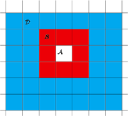
Figure 2: Illustration of $\mathcal{A}$, $\mathcal{B}$ and $\mathcal{D}$.

Further, let

$$b_{0}=u^{-1-d/2}b,\qquad b-b_{0}=(1-u^{-1-d/2})b=e^{-(1+o(1))u^{-1-d/2}}b,$$ (29)

and $u_{0}$ solves

$$u_{0}^{-d/2}e^{\sigma u_{0}+H_{0}}=b_{0},$$

and there exists $c_{0}>0$ such that $u_{0}>u-c_{0}\log u$. The first step in developing the upper bound is to use the following inequality

$$P(\mathcal{A}+\mathcal{B}+\mathcal{D}>b)$$

$$\qquad\leq P(\mathcal{A}>b-b_{0})+P(\mathcal{A}\leq b_{0},\mathcal{A}+\mathcal{B}+\mathcal{D}>b)$$

$$\qquad\quad{}+P(b_{0}<\mathcal{A}\leq b-b_{0},\mathcal{A}+\mathcal{B}+\mathcal{D}>b)$$ (30)

$$\qquad\leq P(\mathcal{A}>b-b_{0})+P(\mathcal{B}+\mathcal{D}>b-b_{0})$$

$$\qquad\quad{}+P(\mathcal{A}>b_{0},\mathcal{B}+\mathcal{D}>b_{0},\mathcal{A}+\mathcal{B}+\mathcal{D}>b).$$

From Theorem 2,

$$P(\mathcal{A}>b-b_{0})=\bigl{(}1+o(1)\bigr{)}P(\mathcal{A}>b).$$

The next step is to show that the last term in (5) is ignorable. Note that

$$P(\mathcal{A}>b_{0},\mathcal{B}+\mathcal{D}>b_{0},\mathcal{A}+\mathcal{B}+\mathcal{D}>b)$$

$$\qquad=P(\mathcal{A}+\mathcal{B}>b-b_{0},\mathcal{A}>b_{0},\mathcal{B}+\mathcal{D}>b_{0},\mathcal{A}+\mathcal{B}+\mathcal{D}>b)$$

$$\qquad\quad{}+P(\mathcal{D}>b-b_{0},\mathcal{A}>b_{0},\mathcal{B}+\mathcal{D}>b_{0},\mathcal{A}+\mathcal{B}+\mathcal{D}>b)$$

$$\qquad\quad{}+P(\mathcal{A}+\mathcal{B}>b_{0},\mathcal{D}>b_{0},\mathcal{A}>b_{0},\mathcal{B}+\mathcal{D}>b_{0},\mathcal{A}+\mathcal{B}+\mathcal{D}>b)$$

$$\qquad\leq P(\mathcal{A}+\mathcal{B}>b-b_{0},\mathcal{A}>b_{0},\mathcal{B}+\mathcal{D}>b_{0},\mathcal{A}+\mathcal{B}+\mathcal{D}>b)$$

$$\qquad\quad{}+2P(\mathcal{D}>b_{0},\mathcal{A}>b_{0})$$

$$\qquad=o\bigl{(}P(\mathcal{A}>b)\bigr{)}.$$

The last step is due to Lemmas 9 and 10. By noting that $\#(\mathcal{C}^{+})u^{-1-d/2}=o(u^{-1})$, the conclusion of the theorem is immediate by induction, where $\#(\cdot)$ is the cardinality of a set.

Appendix: Lemmas in Sections 4 and 5

Lemma 1 isolated the dominating event so that we will be in good shape to use Taylor’s expansion.

Lemma 1

There exist $\varepsilon_{0},\delta>0$ small enough and $\kappa$ large. Let $\varepsilon=\kappa u^{-1/2+\delta}$ such that for any $\alpha>0$,

$$P\biggl{(}|f(0)-u|>u^{2\delta+\varepsilon_{0}}\mbox{ or }|\partial f(0)|>u^{{1}/{2}+\delta+\varepsilon_{0}}\mbox{ or }$$

$$\hskip 21.2pt|\partial^{2}f(0)-u\mu_{20}|>u^{{1}/{2}+\varepsilon_{0}},\int{\Xi_{\varepsilon}}e^{f(t)}\,dt>b\biggr{)}$$

$$\qquad=o(1)u^{-\alpha}e^{-({1}/{2})u^{2}}.$$

Note that there exists $c_{1}$ such that $\sigma u\leq\log b+c_{1}\log\log b$. Let $\sigma\tilde{u}=\log(b)$. Since we only consider the case that $u$ is large, we always have $\operatorname{mes}(\Xi_{\varepsilon})<1$:

$$P\biggl{(}f(0)<u-u^{2\delta+\varepsilon_{0}},\int_{\Xi_{\varepsilon}}e^{f(t)}\,dt>b\biggr{)}$$

$$\qquad\leq P\bigl{(}f(0)<u-u^{2\delta+\varepsilon_{0}},\sup f(t)>\tilde{u}\bigr{)}$$

$$\qquad\leq CP\bigl{(}f(0)<u-u^{2\delta+\varepsilon_{0}}|\sup f(t)>\tilde{u}\bigr{)}\tilde{u}^{d-1}e^{-\tilde{u}^{2}/2}.$$

The last inequality is an application of Proposition 1. Because for any $u^{\prime}>\tilde{u}$, for some $\varepsilon_{1}>0$,

$$\inf_{t\in\Xi_{\varepsilon}}E\Bigl{(}f(t)\big{|}\sup_{\Xi_{\varepsilon}}f(t)=u^{\prime}\Bigr{)}$$

$$\qquad\geq u^{\prime}\inf_{t\in\Xi_{\varepsilon}}C(t)\geq u-\kappa^{2}\varepsilon_{1}u^{2\delta}\bigl{(}1+o(1)\bigr{)}$$

and

$$\sup_{t\in(-\varepsilon,\varepsilon)}\operatorname{Var}\Bigl{(}f(t)\big{|}\sup_{\Xi_{\varepsilon}}f(t)=u^{\prime}\Bigr{)}=O(\varepsilon^{2})=O(u^{-1+2\delta}),$$

one can choose $\kappa$ large enough such that

$$P\Bigl{(}f(0)<u-u^{2\delta+\varepsilon_{0}}\big{|}\sup_{\Xi_{\varepsilon}}f(t)>\tilde{u}\Bigr{)}=O(1)\exp(-{u^{1+\varepsilon_{0}}}/{c_{2}}).$$

Therefore,

$$P\biggl{(}f(0)<u-u^{2\delta+\varepsilon_{0}},\int_{\Xi_{\varepsilon}}e^{f(t)}\,dt>b\biggr{)}=o(1)u^{-\alpha}e^{-u^{2}/2}$$

for all $\alpha>0$. Also, $P(f(0)>u+u^{2\delta+\varepsilon_{0}})=o(1)u^{-\alpha}e^{-({1}/{2})u^{2}}$. Hence,

$$P\biggl{(}|f(0)-u|>u^{2\delta+\varepsilon_{0}},\int_{\Xi_{\varepsilon}}e^{f(t)}\,dt>b\biggr{)}=o(1)u^{-\alpha}e^{-({1}/{2})u^{2}}.$$

Similarly, we have

$$P\biggl{(}|f(0)-u|<u^{2\delta+\varepsilon_{0}},|\partial f(0)|>u^{{1}/{2}+\delta+\varepsilon_{0}},\int_{\Xi_{\varepsilon}}e^{f(t)}\,dt>b\biggr{)}$$

$$\qquad=o(1)u^{-\alpha}e^{-({1}/{2})u^{2}},$$

$$P\biggl{(}|f(0)-u|<u^{2\delta+\varepsilon_{0}},|\partial^{2}f(0)-u\mu_{20}|>u^{{1}/{2}+\varepsilon_{0}},\int_{\Xi_{\varepsilon}}e^{f(t)}\,dt>b\biggr{)}$$

$$\qquad=o(1)u^{-\alpha}e^{-({1}/{2})u^{2}}.$$

The above two displays are immediate by noting that $(f(0),\partial f(0),\partial^{2}f(0))$ is a multivariate Gaussian random vector. In addition, $(f(0),\partial^{2}f(0))$ is independent of $\partial f(0)$ and the covariance between $f(0)$ and $\partial^{2}f(0)$ is $\mu_{02}$.

Lemma 2

Let $h(w,y,z)$ be the density of $(f(0),\partial f(0),\partial^{2}f(0))$. Then,

$$h(w,y,z)$$

$$\qquad=\frac{1}{(2\pi)^{(d+1)(d+2)/4}}|\Gamma|^{-1/2}$$

$$\qquad\quad{}\times\exp\biggl{\{}-\biggl{[}\frac{1}{2}u^{2}+\frac{u}{\sigma}A(w,y,z)+\frac{1}{2}y^{\top}\bigl{(}I-(I-\mathbf{z}/u)^{-1}\bigr{)}y$$

$$\qquad\quad\hskip 47.6pt{}+\frac{1}{2}\frac{(w+\mu_{20}\mu_{22}^{-1}z)^{2}}{1-\mu_{20}\mu_{22}^{-1}\mu_{02}}+\frac{1}{2}z^{\top}\mu_{22}^{-1}z+\frac{u}{2\sigma}\log\det(I-u^{-1}\mathbf{z})$$

$$\qquad\quad\hskip 121.0pt{}-\frac{u}{\sigma}\log\int_{|(uI-\mathbf{z})^{-1/2}t|<\varepsilon}e^{\sigma J(t)}\,dt+uH_{0}/\sigma\biggr{]}\biggr{\}}.$$

In addition,

$$\Gamma^{-1}=\pmatrix{\dfrac{1}{1-\mu_{20}\mu_{22}^{-1}\mu_{02}}&-\dfrac{\mu_{20}\mu_{22}^{-1}}{1-\mu_{20}\mu_{22}^{-1}\mu_{02}}\vspace*{3pt}\cr-\dfrac{\mu_{22}^{-1}\mu_{02}}{1-\mu_{20}\mu_{22}^{-1}\mu_{02}}&\mu_{22}^{-1}+\dfrac{\mu_{22}^{-1}\mu_{02}\mu_{20}\mu_{22}^{-1}}{1-\mu_{20}\mu_{22}^{-1}\mu_{02}}}.$$ (31)

The form of $\Gamma^{-1}$ in (31) is a result from linear algebra. The form of $\Gamma^{-1}$ is direct application of the block matrix inverse from linear algebra. Note that

$$h(w,y,z) = \frac{1}{(2\pi)^{(d+1)(d+2)/4}}|\Gamma|^{-1/2}$$

$${}\times\exp\left\{-\frac{1}{2}(u-w,z^{\top}+u\mu_{20},y^{\top})\pmatrix{\Gamma^{-1}&0\cr 0&I}\pmatrix{u-w\cr z+u\mu_{02}\cr y}\right\}.$$

By plugging in the form of $\Gamma^{-1}$, we have

$$(u-w,z^{\top}+u\mu_{20},y^{\top})\pmatrix{\Gamma^{-1}&0\cr 0&I}\pmatrix{u-w\cr z+u\mu_{02}\cr y}$$

$$\qquad=y^{\top}y+\frac{(u-w)^{2}}{1-\mu_{20}\mu_{22}^{-1}\mu_{02}}$$

$$\qquad\quad{}+(z+u\mu_{02})^{\top}\biggl{[}\mu_{22}^{-1}+\frac{\mu_{22}^{-1}\mu_{02}\mu_{20}\mu_{22}^{-1}}{1-\mu_{20}\mu_{22}^{-1}\mu_{02}}\biggr{]}(z+u\mu_{02})$$

$$\qquad\quad{}-2(u-w)\frac{\mu_{20}\mu_{22}^{-1}}{1-\mu_{20}\mu_{22}^{-1}\mu_{02}}(z+u\mu_{02})$$

$$\qquad=u^{2}+y^{\top}y-2wu+\frac{w^{2}}{1-\mu_{20}\mu_{22}^{-1}\mu_{02}}$$

$$\qquad\quad{}+z^{\top}\biggl{[}\mu_{22}^{-1}+\frac{\mu_{22}^{-1}\mu_{02}\mu_{20}\mu_{22}^{-1}}{1-\mu_{20}\mu_{22}^{-1}\mu_{02}}\biggr{]}z+2w\frac{\mu_{20}\mu_{22}^{-1}}{1-\mu_{20}\mu_{22}^{-1}\mu_{02}}z$$

$$\qquad=u^{2}+\frac{2u}{\sigma}A(w,y,z)+y^{\top}\bigl{(}I-(uI-\mathbf{z})^{-1}\bigr{)}y+\frac{(w+\mu_{20}\mu_{22}^{-1}z)^{2}}{1-\mu_{20}\mu_{22}^{-1}\mu_{02}}$$

$$\qquad\quad{}+z^{\top}\mu_{22}^{-1}z+\frac{u}{\sigma}\log\det(I-u^{-1}\mathbf{z})$$

$$\qquad\quad{}-\frac{2u}{\sigma}\log\int_{|(uI-\mathbf{z})^{-1/2}t|<\varepsilon}e^{J(t)}\,dt+\frac{2u}{\sigma}H_{0}.$$

Therefore, we conclude the proof.

Lemma 3

$$\log\bigl{(}\det(I-u^{-1}\mathbf{z})\bigr{)}=-u^{-1}\operatorname{Tr}(\mathbf{z})+\tfrac 12u^{-2}\mathcal{E}^{2}(\mathbf{z})+o(u^{-2}),$$

where $\mathrm{Tr}$ is the trace of a matrix, $\mathcal{E}^{2}(\mathbf{z})=\sum_{i=1}^{d}\lambda_{i}^{2}$, and $\lambda_{i}$’s are the eigenvalues of $\mathbf{z}$.

The result is immediate by noting that

$$\det(I-u^{-1}\mathbf{z})=\prod_{i=1}^{d}(1-\lambda_{i}/u)$$

and $\operatorname{Tr}(\mathbf{z})=\sum_{i=1}^{d}\lambda_{i}$.

Lemma 4

Let $y=(y_{1},\ldots,y_{d})^{\top}$ and $X\sim N(y/\sqrt{u},I/\sqrt{\sigma})$. Then, on the set $\mathcal{L}$ defined in (20),

$$E\bigl{(}g_{3}\bigl{(}X/\sqrt{u}\bigr{)}+g_{4}\bigl{(}X/\sqrt{u}\bigr{)}\bigr{)}$$

$$\qquad=-\frac{u^{-1}}{8}(u^{-1}Y+\mathbf{1}/\sigma)^{\top}\mu_{22}(u^{-1}Y+\mathbf{1}/\sigma)$$

$$\qquad\quad{}+\frac{u^{-1}}{8\sigma^{2}}\mathbf{1}^{\top}\mu_{22}\mathbf{1}+\frac{u^{-1}}{8\sigma^{2}}\sum_{i}\partial_{iiii}C(0)+o(u^{-1}),$$

where

$$Y = (y_{i}^{2},i=1,\ldots,d,2y_{i}y_{j},1\leq i<j\leq d)^{\top},$$

$$\mathbf{1} = (\underbrace{1,\ldots,1}_{d},\underbrace{0,\ldots,0}_{d(d-1)/2})^{\top}.$$

Using the derivatives in (2.1), we have that

$$\partial_{ijk}E(0) = -\sum_{l=1}^{d}\partial^{4}_{ijkl}C(0)y_{l},$$

$$\partial^{4}_{ijk}E(0) = \bigl{(}u+O(|z|+|w|)\bigr{)}\partial_{ijkl}C(0).$$

We plug this into the definition of $g_{3}$ and $g_{4}$ in (6) and obtain, on the set $\mathcal{L}$,

$$E\bigl{(}g_{3}\bigl{(}X/\sqrt{u}\bigr{)}+g_{4}\bigl{(}X/\sqrt{u}\bigr{)}\bigr{)}$$

$$\qquad=-\frac{1}{6}u^{-3/2}\sum_{ijkl}\partial^{4}_{ijkl}C(0)E(X_{i}X_{j}X_{k}y_{l})$$

$$\qquad\quad{}+\frac{u^{-1}}{24}\sum_{ijkl}\partial^{4}_{ijkl}C(0)E(X_{i}X_{j}X_{k}X_{l})+o(u^{-1})$$

$$\qquad=-\frac{1}{8}u^{-3/2}\sum_{ijkl}\partial^{4}_{ijkl}C(0)E(X_{i}X_{j}X_{k}y_{l})$$

$$\qquad\quad{}+\frac{u^{-1}}{24}\sum_{ijkl}\partial^{4}_{ijkl}C(0)E\bigl{(}X_{i}X_{j}X_{k}\bigl{(}X_{l}-y_{l}/\sqrt{u}\bigr{)}\bigr{)}+o(u^{-1})$$

$$\qquad=-\frac{1}{8}u^{-3}\sum_{ijkl}\partial^{4}_{ijkl}C(0)y_{i}y_{j}y_{k}y_{l}-\frac{3}{8\sigma}u^{-2}\sum_{il}y_{i}y_{l}\sum_{j}\partial^{4}_{iljj}C(0)$$

$$\qquad\quad{}+\frac{u^{-2}}{8\sigma}\sum_{ij}y_{i}y_{j}\sum_{l}\partial^{4}_{ijll}C(0)+\frac{3u^{-1}}{24\sigma^{2}}\sum_{i}\partial^{4}_{iiii}C(0)+o(u^{-1})$$

$$\qquad=-\frac{1}{8}u^{-3}\sum_{ijkl}\partial^{4}_{ijkl}C(0)y_{i}y_{j}y_{k}y_{l}-\frac{1}{4\sigma}u^{-2}\sum_{ij}y_{i}y_{j}\sum_{l}\partial^{4}_{ijll}C(0)$$

$$\qquad\quad{}+\frac{u^{-1}}{8\sigma^{2}}\sum_{i}\partial^{4}_{iiii}C(0)+o(u^{-1}).$$

This last step is true because $\sum_{il}y_{i}y_{l}\sum_{j}\partial^{4}_{iljj}C(0)=\sum_{ij}y_{i}y_{j}\sum_{l}\partial^{4}_{ijll}C(0)$, which is just a change of index. Then, with the definition of $Y$ and $\mathbf{1}$ in the statement of this lemma (note that $\mathbf{1}$ is NOT a vector of $1$’s), we have

$$E\bigl{(}g_{3}\bigl{(}X/\sqrt{u}\bigr{)}+g_{4}\bigl{(}X/\sqrt{u}\bigr{)}\bigr{)}$$

$$\qquad=-\frac{u^{-3}}{8}Y^{\top}\mu_{22}Y-\frac{u^{-2}}{4\sigma}Y^{\top}\mu_{22}\mathbf{1}+\frac{u^{-1}}{8\sigma^{2}}\sum_{i}\partial^{4}_{iiii}C(0)+o(1)$$

$$\qquad=-\frac{u^{-1}}{8}(u^{-1}Y+\mathbf{1}/\sigma)^{\top}\mu_{22}(u^{-1}Y+\mathbf{1}/\sigma)+\frac{u^{-1}}{8\sigma^{2}}\mathbf{1}^{\top}\mu_{22}\mathbf{1}$$

$$\qquad\quad{}+\frac{u^{-1}}{8\sigma^{2}}\sum_{i}\partial^{4}_{iiii}C(0)+o(1).$$

Lemma 5

Let $J(t)$ be defined in (4). Then, on the set $\mathcal{L}$ the approximations of $\int_{|(uI-\mathbf{z})^{-1/2}t|_{\infty}<\varepsilon}e^{\sigma J(t)}\,dt$ under different situations are as follows: [(2)]

When $|(uI-\mathbf{z})^{-1/2}y|_{\infty}\leq\kappa u^{\delta}-u^{\delta/2}$,

$$\int_{|(uI-\mathbf{z})^{-1/2}t|_{\infty}<\varepsilon}e^{\sigma J(t)}\,dt$$

$$\qquad=\exp\bigl{[}\sigma E\bigl{(}g_{3}\bigl{(}X/\sqrt{u}\bigr{)}+g_{4}\bigl{(}X/\sqrt{u}\bigr{)}\bigr{)}$$

$$\qquad\quad\hskip 17.6pt{}+H\bigl{(}(uI-\mathbf{z})^{-1/2}y,(uI-\mathbf{z})^{1/2},\varepsilon\bigr{)}+o(u^{-1})\bigr{]},$$

where

$$e^{H(y,\Sigma,\varepsilon)}=\int_{|\Sigma^{-1}t|<\varepsilon}e^{-({\sigma}/{2})(t-y)^{\top}(t-y)}\,dt,$$

and $X$ is the random vector defined in Lemma 4. In addition,

$$H\bigl{(}0,(uI-\mathbf{z})^{1/2},\varepsilon\bigr{)}-H_{0}=o(u^{-1}).$$

For any $\varepsilon_{1}>0$, when $\kappa u^{\delta}-u^{\delta/2}\leq|(uI-\mathbf{z})^{-1/2}y|_{\infty}\leq(1+\varepsilon_{1})\kappa u^{\delta}$,

$$\int_{|(uI-\mathbf{z})^{-1/2}t|<\varepsilon}e^{\sigma J(t)}\,dt$$

$$\qquad\leq\exp\bigl{[}\sigma E\bigl{(}g_{3}\bigl{(}X/\sqrt{u}\bigr{)}+g_{4}\bigl{(}X/\sqrt{u}\bigr{)}\bigr{)}$$

$$\qquad\quad\hskip 17.0pt{}+H\bigl{(}(uI-\mathbf{z})^{-1/2}y,(uI-\mathbf{z})^{1/2},\varepsilon\bigr{)}+o(u^{-1})\bigr{]}.$$

When $(1+\varepsilon_{1})\kappa u^{\delta}<|(uI-\mathbf{z})^{-1/2}y|_{\infty}\leq u^{\delta+\varepsilon_{0}}$

$$\int_{|(uI-\mathbf{z})^{-1/2}t|<\varepsilon}e^{\sigma J(t)}\,dt$$

$$\qquad\leq\frac{1}{2}\exp\bigl{[}\sigma E\bigl{(}g_{3}\bigl{(}X/\sqrt{u}\bigr{)}+g_{4}\bigl{(}X/\sqrt{u}\bigr{)}\bigr{)}+H_{0}+o(u^{-1})\bigr{]}.$$

Note that

$$\int_{|(uI-\mathbf{{\mathbf{z}}})^{-1/2}t|<\varepsilon}e^{\sigma J(t)}\,dt$$

$$\qquad=e^{H((uI-{\mathbf{z}})^{-1/2}y,(uI-{\mathbf{z}})^{-1/2},\varepsilon)}$$

$$\qquad\quad{}\times E\bigl{\{}\exp\bigl{[}\sigma g_{3}\bigl{(}(uI-{\mathbf{z}})^{-1/2}X^{\prime}\bigr{)}$$

$$\qquad\quad\hskip 24.0pt{}+\sigma g_{4}\bigl{(}(uI-{\mathbf{z}})^{-1/2}X^{\prime}\bigr{)}+\sigma R\bigl{(}(uI-{\mathbf{z}})^{-1/2}X^{\prime}\bigr{)}\bigr{]};$$

$$\qquad\quad\hskip 149.2pt|(uI-\mathbf{{\mathbf{z}}})^{-1/2}X^{\prime}|<\varepsilon\bigr{\}}.$$

Also, $(uI-{\mathbf{z}})^{-1/2}X^{\prime}=(1+O(z/u))X^{\prime}/\sqrt{n}$ and

$$X^{\prime}=X-y/\sqrt{u}+(uI-{\mathbf{z}})^{-1/2}y=X+O(u^{-3/2})|{\mathbf{z}}y|.$$

For the first situation, $|(uI-{\mathbf{z}})^{-1/2}y|_{\infty}\leq\kappa u^{\delta}-u^{\delta/2}$ and $|z|<u^{1/2+\varepsilon_{0}}$,

$$E\bigl{\{}\exp\bigl{[}\sigma g_{3}\bigl{(}(uI-{\mathbf{z}})^{-1/2}X^{\prime}\bigr{)}+\sigma g_{4}\bigl{(}(uI-{\mathbf{z}})^{-1/2}X^{\prime}\bigr{)}+\sigma R\bigl{(}(uI-{\mathbf{z}})^{-1/2}X^{\prime}\bigr{)}\bigr{]};$$

$$\hskip 252.8pt|(uI-\mathbf{z})^{-1/2}X^{\prime}|<\varepsilon\bigr{\}}$$

$$\qquad=E\bigl{\{}\exp\bigl{[}\sigma g_{3}\bigl{(}X^{\prime}/\sqrt{u}\bigr{)}+\sigma g_{4}\bigl{(}X^{\prime}/\sqrt{u}\bigr{)}+\sigma R\bigl{(}X^{\prime}/\sqrt{u}\bigr{)}+o(u^{-1})\bigr{]};$$

$$\hskip 219.2pt|(uI-\mathbf{z})^{-1/2}X^{\prime}|<\varepsilon\bigr{\}}$$

$$\qquad=E\bigl{\{}\exp\bigl{[}\sigma g_{3}\bigl{(}X^{\prime}/\sqrt{u}\bigr{)}+\sigma g_{4}\bigl{(}X^{\prime}/\sqrt{u}\bigr{)}+\sigma R\bigl{(}X^{\prime}/\sqrt{u}\bigr{)}+o(u^{-1})\bigr{]}\bigr{\}}$$

$$\qquad=E\bigl{\{}\exp\bigl{[}\sigma g_{3}\bigl{(}X/\sqrt{u}\bigr{)}+\sigma g_{4}\bigl{(}X/\sqrt{u}\bigr{)}+\sigma R\bigl{(}X/\sqrt{u}\bigr{)}+o(u^{-1})\bigr{]}\bigr{\}}.$$

In addition, because $|R(t)|=O(u^{1/2+\delta}t^{5})$, then

$$E\bigl{\{}\exp\bigl{[}\sigma g_{3}\bigl{(}X/\sqrt{u}\bigr{)}+\sigma g_{4}\bigl{(}X/\sqrt{u}\bigr{)}+\sigma R\bigl{(}X/\sqrt{u}\bigr{)}\bigr{]}\bigr{\}}$$

$$\qquad=E\bigl{\{}\exp\bigl{[}\sigma g_{3}\bigl{(}X/\sqrt{u}\bigr{)}+\sigma g_{4}\bigl{(}X/\sqrt{u}\bigr{)}+o(u^{-1})\bigr{]}\bigr{\}}.$$

Further, $g_{3}(X/\sqrt{u})=o(u^{-1/2+\delta})$ and $g_{4}(X/\sqrt{u})=o(u^{-1/2+\delta})$, then by repeatedly using Talyor’s expansion, we have

$$E\bigl{\{}\exp\bigl{[}\sigma g_{3}\bigl{(}X^{\prime}/\sqrt{u}\bigr{)}+\sigma g_{4}\bigl{(}X^{\prime}/\sqrt{u}\bigr{)}+\sigma R\bigl{(}X^{\prime}/\sqrt{u}\bigr{)}\bigr{]};|(uI-\mathbf{z})^{-1/2}X^{\prime}|<\varepsilon\bigr{\}}$$

$$\qquad=\exp\bigl{\{}E\bigl{[}\sigma g_{3}\bigl{(}X/\sqrt{u}\bigr{)}+\sigma g_{4}\bigl{(}X/\sqrt{u}\bigr{)}+o(u^{-1})\bigr{]}\bigr{\}}.$$

For the second situation, the inequality is immediate by noting that

$$E\bigl{\{}\exp\bigl{[}\sigma g_{3}\bigl{(}X^{\prime}/\sqrt{u}\bigr{)}+\sigma g_{4}\bigl{(}X^{\prime}/\sqrt{u}\bigr{)}+\sigma R\bigl{(}X^{\prime}/\sqrt{u}\bigr{)}\bigr{]};|(uI-\mathbf{z})^{-1/2}X^{\prime}|<\varepsilon\bigr{\}}$$

$$\qquad\leq E\bigl{\{}\exp\bigl{[}\sigma g_{3}\bigl{(}X^{\prime}/\sqrt{u}\bigr{)}+\sigma g_{4}\bigl{(}X^{\prime}/\sqrt{u}\bigr{)}+\sigma R\bigl{(}X^{\prime}/\sqrt{u}\bigr{)}\bigr{]}\bigr{\}}.$$

For the third situation, note that the integral is not focusing on the dominating part, and the conclusion follows immediately.

The next lemma is known as the Borel-TIS lemma, which was proved independently by Bor75 , CIS .

Lemma 6 ((Borel-TIS))

Let $f(t)$, $t\in\mathcal{U}$, $\mathcal{U}$ is a parameter set, be a mean zero Gaussian random field. $f$ is almost surely bounded on $\mathcal{U}$. Then,

$$E\Bigl{(}\sup_{\mathcal{U}}f(t)\Bigr{)}<\infty$$

and

$$P\Bigl{(}\max_{t\in\mathcal{U}}f(t)-E\Bigl{[}\max_{t\in\mathcal{U}}f(t)\Bigr{]}\geq b\Bigr{)}\leq e^{-{b^{2}}/({2\sigma_{\mathcal{U}}^{2}})},$$

where

$$\sigma_{\mathcal{U}}^{2}=\max_{t\in\mathcal{U}}\operatorname{Var}[f(t)].$$

Lemma 7

Let $\log E\exp(g((uI-\mathbf{z})^{-1/2}S))$ be defined in (17), then there exists a $\lambda>0$ such that for all $x>0$

$$P\bigl{(}u^{-3/2-3\delta}\bigl{|}\log E\exp\bigl{(}\sigma g\bigl{(}(uI-\mathbf{z})^{-1/2}S\bigr{)}\bigr{)}\bigr{|}>x\bigr{)}\leq e^{-\lambda x^{2}}$$

for $u$ sufficiently large.

Note that $g(t)$ is a mean zero Gaussian random field with $\operatorname{Var}(g(t))=O(|t|^{6})$ and $|S|\leq\kappa u^{\delta}$. A direct application of the Borel-TIS lemma yields the result of this lemma.

Lemma 8

For each $\mathbf{k}\neq\mathbf{k}^{\prime}$,

$$P\bigl{(}I_{\sigma}(\Xi_{\varepsilon,\mathbf{k}})>b,I_{\sigma}(\Xi_{\varepsilon,\mathbf{k}^{\prime}})>b\bigr{)}=O(1)u^{d-1}e^{-u^{2}/2-\Theta(u)}.$$

Without loss of generality, we consider $\Xi_{\varepsilon,\mathbf{k}^{\prime}}=\Xi_{\varepsilon}$. If $\Xi_{\varepsilon}$ and $\Xi_{\varepsilon,\mathbf{k}^{\prime}}$ are connected to each other,

$$P\bigl{(}I_{\sigma}(\Xi_{\varepsilon,\mathbf{k}})>b,I_{\sigma}(\Xi_{\varepsilon})>b\bigr{)} \leq P\bigl{(}I_{\sigma}(\Xi_{\varepsilon}\cup\Xi_{\varepsilon,\mathbf{k}})>2b\bigr{)}$$

$$= O(1)m(\Xi_{\varepsilon})u^{d-1}e^{-(1/2)(u+\log 2+o(1))^{2}}$$

$$= O(1)u^{d-1}e^{-({1/2})u^{2}-(\log 2+o(1))u}.$$

The second step is an application of Theorem 2. If $\Xi_{\varepsilon}$ and $\Xi_{\varepsilon,\mathbf{k}^{\prime}}$ are not connected, that is, $\inf_{s\in\Xi_{\varepsilon},t\in\Xi_{\varepsilon,\mathbf{k}^{\prime}}}|s-t|\geq\varepsilon=\kappa u^{-1/2+\delta}$, then

$$P\bigl{(}I_{\sigma}(\Xi_{\varepsilon,\mathbf{k}})>b,I_{\sigma}(\Xi_{\varepsilon})>b\bigr{)}$$

$$\qquad\leq P\Bigl{(}\sup_{t\in\Xi_{\varepsilon}}f(t)>u-c\log u,\sup_{t\in\Xi_{\varepsilon,\mathbf{k}}}f(t)>u-c\log u\Bigr{)}$$

$$\qquad\leq P\Bigl{(}\sup_{t\in\Xi_{\varepsilon},s\in\Xi_{\varepsilon,\mathbf{k}}}f(t)+f(s)>2u-2c\log u\Bigr{)}$$

$$\qquad\leq O(1)P\biggl{(}Z>\frac{2u-2c\log u+O(1)}{\sqrt{4-\Theta(1)u^{-1+2\delta}}}\biggr{)}$$

$$\qquad=O(1)u^{d-1}e^{-({1/2})u^{2}-\Theta(1)u^{1+2\delta}},$$

where $Z$ is a standard Gaussian random variable. The last inequality is an application of the Borel-TIS lemma in Lemma 6.

Lemma 9

Let $\mathcal{A}$ and $\mathcal{D}$ be defined in (28) and $b_{0}$ be defined in (29). Then,

$$P(\mathcal{D}>b_{0},\mathcal{A}>b_{0})=o\bigl{(}P(\mathcal{A}>b)\bigr{)}.$$

Similar to the second case in the proof of Lemma 8, we have

$$P(D>b_{0},A>b_{0})$$

$$\qquad\leq P\Bigl{(}\sup_{\Xi_{\varepsilon}}f(t)>u-c_{1}\log u,\sup_{\bigcup_{\mathbf{k}\in C^{+}\setminus\{\mathbf{0},\mathbf{k}\}}\Xi_{\varepsilon,\mathbf{k}}}f(t)>u-c_{1}\log u\Bigr{)}$$

$$\qquad\leq P\Bigl{(}\sup_{s\in\Xi_{\varepsilon},t\in\bigcup_{\mathbf{k}\in C^{+}\setminus\{\mathbf{0},\mathbf{k}\}}\Xi_{\varepsilon,\mathbf{k}}}f(s)+f(t)>2u-2c_{1}\log u\Bigr{)}$$

$$\qquad\leq u^{\alpha}e^{-{(2u-2c_{1}\log u)^{2}}/({2(4-2\kappa^{2}u^{-1+2\delta})})}\leq e^{-{u^{2}}/{2}-\Theta(1)u^{1+2\delta}}.$$

The conclusion follows immediately.

Lemma 10

Let $\mathcal{A}$, $\mathcal{B}$ and $\mathcal{D}$ be defined in (28) and $b_{0}$ be defined in (29). Then,

$$P(\mathcal{A}+\mathcal{B}>b-b_{0},\mathcal{A}>b_{0},\mathcal{B}+\mathcal{D}>b_{0})=o(1)P(\mathcal{A}>b).$$

Note that there exists $c^{\prime}>0$ such that

$$P(\mathcal{A}+\mathcal{B}>b-b_{0},\mathcal{A}>b_{0},\mathcal{B}+\mathcal{D}>b_{0})$$

$$\qquad\leq P\Bigl{(}\mathcal{A}+\mathcal{B}>b-b_{0},\sup_{\Xi_{\varepsilon}}f(t)>u-c^{\prime}\log u,$$

$$\qquad\hskip 65.3pt\sup_{\bigcup_{\mathbf{k}\in\mathcal{C}^{+}\setminus\{\mathbf{0}\}}\Xi_{\varepsilon,\mathbf{k}}}f(t)>u-c^{\prime}\log u\Bigr{)}.$$

It suffices to show that the right-hand side of the above inequality is$o(1)P(\mathcal{A}>b)$ and also $o(1)P(\mathcal{A}+\mathcal{B}>b)$. In order to do so, we will borrow part of the derivations in the proof of Theorem 2. Let $u_{*}$ solve

$$(2\pi/\sigma)^{d/2}u_{*}^{-d/2}e^{\sigma u_{*}}=b-b_{0}.$$

Note that because $b_{0}=u^{-1-d/2}b$, we have $|u-u_{*}|=o(u^{-1})$ and $e^{-u^{2}/2}=(1+o(1))e^{-u_{*}^{2}/2}$. By the results in (4), (4) and (4), we have

$$P\Bigl{(}\mathcal{A}+\mathcal{B}>b-b_{0},\sup_{\Xi_{\varepsilon}}f(t)>u-c^{\prime}\log u,\sup_{\bigcup_{\mathbf{k}\in\mathcal{C}^{+}\setminus\{\mathbf{0}\}}\Xi_{\varepsilon,\mathbf{k}}}f(t)>u-c^{\prime}\log u\Bigr{)}$$

$$\qquad=o(1)P(\mathcal{A}+\mathcal{B}>b-b_{0})$$

$$\qquad\quad{}+\bigl{(}1+o(1)\bigr{)}\sigma^{-1}\det(\Gamma)^{-1/2}\det(\mu_{22})^{1/2}u^{-1}$$

$$\hskip 11.0pt\qquad\quad{}\times e^{-({1/2})u^{2}+({1}/({8\sigma^{2}}))\mathbf{1}^{\top}\mu_{22}\mathbf{1}+({1}/({8\sigma^{2}}))\sum_{i}\partial_{iiii}C(0)}$$

$$\hskip 11.0pt\qquad\quad{}\times\int_{\{|y|_{\infty}\leq 3\kappa u^{1/2+\delta}\}}P\Bigl{(}A^{\prime}>o_{p}(1),\sup_{\Xi_{\varepsilon}}E(t)+g(t)>u_{\ast}-c^{\prime}\log u_{\ast},$$

$$\qquad\quad\hskip 125.2pt\sup_{\bigcup_{\mathbf{k}\in\mathcal{C}^{+}\setminus\{\mathbf{0}\}}\Xi_{\varepsilon,\mathbf{k}}}E(t)+g(t)>u_{\ast}-c^{\prime}\log u_{\ast}\Bigr{)}$$

$$\qquad\quad\hskip 11.0pt{}\times\exp\biggl{\{}-\biggl{[}\frac{A^{\prime}}{\sigma}+\frac{B^{\top}B}{2}$$

$$\qquad\quad\hskip 57.0pt{}+\frac{(-{A^{\prime}}/({\sigma u})+\mu_{20}\mu_{22}^{-1/2}B+({1}/({2\sigma}))\mu_{20}\mathbf{1})^{2}}{2(1-\mu_{20}\mu_{22}^{-1}\mu_{02})}\biggr{]}\biggr{\}}\,dA^{\prime}\,dB\,dy.$$

Note that the only change in the above display from (4) is the probability inside the integral. In what follows, we show that it is almost always $o(1)$. Note that $\operatorname{Var}(g(t))=O(|t|^{6})$. Therefore, for any $f(0)<u+u^{\varepsilon_{0}}$ with $\varepsilon_{0}<\delta/2$, if

$$\sup_{\Xi_{\varepsilon}}E(t) < u-c^{\prime}\log u-\Theta(u^{-1})\quad\mbox{or }$$

$$\sup_{\Xi_{3\varepsilon}\setminus\Xi_{\varepsilon}}E(t) < u-c^{\prime}\log u-\Theta(u^{-1}),$$

then

$$P\Bigl{(}\sup_{\Xi_{\varepsilon}}E(t)+g(t)>u-c^{\prime}\log u,\sup_{\bigcup_{\mathbf{k}\in\mathcal{C}^{+}\setminus\{\mathbf{0}\}}\Xi_{\varepsilon,\mathbf{k}}}E(t)+g(t)>u-c^{\prime}\log u\Bigr{)}=o(1).$$

This fact implies that $g(t)$ can be basically ignored. Therefore, it is useful to keep in mind that “$E(t)\approx f(t)$.”

Since

$$P\Bigl{(}\sup_{T}f(t)>u+u^{-1+\varepsilon_{0}}\Bigr{)}=o(1)P(\mathcal{A}+\mathcal{B}>b-b_{0}),$$

we only need to consider the case that $\sup_{T}E(t)\leq u+u^{-1+\varepsilon_{0}}$. Given the form

$$E(t)=u_{*}-w+y^{\top}t+\tfrac{1}{2}t^{\top}(-u_{*}I+\mathbf{z})t+g_{3}(t)+g_{4}(t)+R(t),$$

which is asymptotically quadratic in $\Xi_{3\varepsilon}$, let $t^{*}=\arg\sup_{\Xi_{3\varepsilon}}E(t)$. On the set that $\sup_{T}E(t)\leq u+u^{-1+\varepsilon_{0}}$, we have

$$\sup_{|t-t^{*}|>2u^{-1/2+\varepsilon_{0}/2}}E(t)<u-c^{\prime}\log u-\Theta(u^{-1}).$$

Let $\partial\Xi_{\varepsilon}$ be the border of $\Xi_{\varepsilon}$. Then

$$\sup_{\Xi_{\varepsilon}}E(t) > u-c^{\prime}\log u-\Theta(u^{-1})\quad\mbox{and}$$

$$\sup_{\Xi_{3\varepsilon}\setminus\Xi_{\varepsilon}}E(t) > u-c^{\prime}\log u-\Theta(u^{-1}),$$

only when $\inf_{t\in\partial\Xi_{\varepsilon}}|t-t^{*}|<u_{*}^{-1/2+\varepsilon_{0}}$. This implies that

$$\inf_{t\in\partial\Xi_{\varepsilon}}|t-(u_{*}I-\mathbf{z})^{-1}y|<u_{*}^{-1/2+\varepsilon_{0}}.$$

Therefore, $t^{*}=\arg\sup f(t)$ must be very closed to the boundary of $\Xi_{\varepsilon}$ so as to have (Appendix: Lemmas in Sections 4 and 5) hold.

Therefore, for all $\varepsilon_{0}<\delta$

$$P\Bigl{(}\mathcal{A}+\mathcal{B}>b-b_{0},\sup_{\Xi_{\varepsilon}}f(t)>u-c^{\prime}\log u,$$

$$\qquad\hskip 2.0pt\sup_{\bigcup_{\mathbf{k}\in\mathcal{C}^{+}\setminus\{\mathbf{0}\}}\Xi_{\varepsilon,\mathbf{k}}}E(t)+g(t)>u-c^{\prime}\log u\Bigr{)}$$

$$\qquad=o(1)P(\mathcal{A}+\mathcal{B}>b-b_{0})$$

$$\qquad\quad{}+\bigl{(}1+o(1)\bigr{)}\sigma^{-1}\det(\Gamma)^{-1/2}\det(\mu_{22})^{1/2}u^{-1}$$

$$\qquad\qquad{}\times e^{-({1/2})u^{2}+({1}/({8\sigma^{2}}))\mathbf{1}^{\top}\mu_{22}\mathbf{1}+({1}/({8\sigma^{2}}))\sum_{i}\partial_{iiii}C(0)}$$

$$\qquad\qquad{}\times\int_{\inf_{t\in\partial\Xi_{\varepsilon}}|t-(u_{\ast}I-\mathbf{z})^{-1}y|<u_{\ast}^{-1/2+\varepsilon_{0}}}P\Bigl{(}A^{\prime}>o_{p}(1),$$

$$\hskip 198.0pt\sup_{\Xi_{\varepsilon}}E(t)+g(t)>u-c^{\prime}\log u,$$

$$\hskip 163.0pt\sup_{\bigcup_{\mathbf{k}\in\mathcal{C}^{+}\setminus\{\mathbf{0}\}}\Xi_{\varepsilon,\mathbf{k}}}E(t)+g(t)>u-c^{\prime}\log u\Bigr{)}$$

$$\qquad\qquad{}\times\exp\biggl{\{}-\biggl{[}\frac{A^{\prime}}{\sigma}+\frac{B^{\top}B}{2}$$

$$\qquad\quad\hskip 54.0pt{}+\frac{(-{A^{\prime}}/({\sigma u})+\mu_{20}\mu_{22}^{-1/2}B+({1}/({2\sigma}))\mu_{20}\mathbf{1})^{2}}{2(1-\mu_{20}\mu_{22}^{-1}\mu_{02})}\biggr{]}\biggr{\}}\,dA^{\prime}\,dB\,dy$$

$$\qquad=o(1)P(\mathcal{A}+\mathcal{B}>b-b_{0}).$$

The last equation is because

$$\operatorname{mes}\Bigl{(}\Bigl{\{}y\dvtx{\inf_{t\in\partial\Xi_{\varepsilon}}}|t-(u_{\ast}I-\mathbf{z})^{-1}y|<u_{\ast}^{-1/2+\varepsilon_{0}}\Bigr{\}}\Bigr{)}$$

$$\qquad=o\bigl{(}\operatorname{mes}\bigl{(}\{y\dvtx|(uI-\mathbf{z})^{-1/2}y|_{\infty}\leq\kappa u^{\delta}-u^{\delta/2}\}\bigr{)}\bigr{)}.$$

Hereby, we conclude the proof.

References

• (1) {bbook}[mr] \bauthor\bsnmAdler, \bfnmRobert J.\binitsR. J. (\byear1981). \btitleThe Geometry of Random Fields. \bpublisherWiley, \baddressChichester. \bidmr=0611857 \endbibitem
• (2) {bmisc}[auto:STB—2011-03-03—12:04:44] \bauthor\bsnmAdler, \bfnmR. J.\binitsR. J., \bauthor\bsnmBlanchet, \bfnmJ. H.\binitsJ. H. and \bauthor\bsnmLiu, \bfnmJ. C.\binitsJ. C. (\byear2008). \bhowpublishedEfficient simulation for tail probabilities of Gaussian random fields. In Proceedings of the 40th Winter Simulation Conference (Miami, Florida) 328–336. \endbibitem
• (3) {bmisc}[auto:STB—2011-03-03—12:04:44] \bauthor\bsnmAdler, \bfnmR. J.\binitsR. J., \bauthor\bsnmBlanchet, \bfnmJ. H.\binitsJ. H. and \bauthor\bsnmLiu, \bfnmJ. C.\binitsJ. C. (\byear2009). \bhowpublishedEfficient Monte Carlo for large excursions of Gaussian random fields. Preprint. \endbibitem
• (4) {bmisc}[auto:STB—2011-03-03—12:04:44] \bauthor\bsnmAdler, \bfnmR. J.\binitsR. J., \bauthor\bsnmSamorodnitsky, \bfnmG.\binitsG. and \bauthor\bsnmTaylor, \bfnmJ. E.\binitsJ. E. (\byear2009). \bhowpublishedHigh level excursion set geometry for non-Gaussian infinitely divisible random fields. Preprint. \endbibitem
• (5) {bbook}[mr] \bauthor\bsnmAdler, \bfnmRobert J.\binitsR. J. and \bauthor\bsnmTaylor, \bfnmJonathan E.\binitsJ. E. (\byear2007). \btitleRandom Fields and Geometry. \bpublisherSpringer, \baddressNew York. \bidmr=2319516 \endbibitem
• (6) {bmisc}[auto:STB—2011-03-03—12:04:44] \bauthor\bsnmAdler, \bfnmR. J.\binitsR. J., \bauthor\bsnmTaylor, \bfnmJ. E.\binitsJ. E. and \bauthor\bsnmWorsley, \bfnmK. J.\binitsK. J. (\byear2009). \bhowpublishedApplications of RANDOM FIELDS AND GEOMETRY: Foundations and case studies. Preprint. \endbibitem
• (7) {barticle}[auto:STB—2011-03-03—12:04:44] \bauthor\bsnmAhsan, \bfnmS. M.\binitsS. M. (\byear1978). \btitlePortfolio selection in a lognormal securities market. \bjournalJournal of Economics \bvolume38 \bpages105–118. \endbibitem
• (8) {barticle}[mr] \bauthor\bsnmAsmussen, \bfnmSøren\binitsS. and \bauthor\bsnmRojas-Nandayapa, \bfnmLeonardo\binitsL. (\byear2008). \btitleAsymptotics of sums of lognormal random variables with Gaussian copula. \bjournalStatist. Probab. Lett. \bvolume78 \bpages2709–2714. \biddoi=10.1016/j.spl.2008.03.035, issn=0167-7152, mr=2465111 \endbibitem
• (9) {barticle}[mr] \bauthor\bsnmAzaïs, \bfnmJean-Marc\binitsJ.-M. and \bauthor\bsnmWschebor, \bfnmMario\binitsM. (\byear2005). \btitleOn the distribution of the maximum of a Gaussian field with $d$ parameters. \bjournalAnn. Appl. Probab. \bvolume15 \bpages254–278. \biddoi=10.1214/105051604000000602, issn=1050-5164, mr=2115043 \endbibitem
• (10) {barticle}[mr] \bauthor\bsnmAzaïs, \bfnmJean-Marc\binitsJ.-M. and \bauthor\bsnmWschebor, \bfnmMario\binitsM. (\byear2008). \btitleA general expression for the distribution of the maximum of a Gaussian field and the approximation of the tail. \bjournalStochastic Process. Appl. \bvolume118 \bpages1190–1218. \biddoi=10.1016/j.spa.2007.07.016, issn=0304-4149, mr=2428714 \endbibitem
• (11) {bbook}[mr] \bauthor\bsnmAzaïs, \bfnmJean-Marc\binitsJ.-M. and \bauthor\bsnmWschebor, \bfnmMario\binitsM. (\byear2009). \btitleLevel Sets and Extrema of Random Processes and Fields. \bpublisherWiley, \baddressHoboken, NJ. \biddoi=10.1002/9780470434642, mr=2478201 \endbibitem
• (12) {barticle}[auto:STB—2011-03-03—12:04:44] \bauthor\bsnmBasak, \bfnmS.\binitsS. and \bauthor\bsnmShapiro, \bfnmA.\binitsA. (\byear2001). \btitleValue-at-risk-based risk management: Optimal policies and asset prices. \bjournalReview of Financial Studies \bvolume14 \bpages371–405. \endbibitem
• (13) {barticle}[mr] \bauthor\bsnmBerman, \bfnmSimeon M.\binitsS. M. (\byear1985). \btitleAn asymptotic formula for the distribution of the maximum of a Gaussian process with stationary increments. \bjournalJ. Appl. Probab. \bvolume22 \bpages454–460. \bidissn=0021-9002, mr=0789369 \endbibitem
• (14) {barticle}[auto:STB—2011-03-03—12:04:44] \bauthor\bsnmBlack, \bfnmF.\binitsF. and \bauthor\bsnmScholes, \bfnmM.\binitsM. (\byear1973). \btitlePricing of options and corporate liabilities. \bjournalJournal of Political Economy \bvolume81 \bpages637–654. \endbibitem
• (15) {bmisc}[auto:STB—2011-03-03—12:04:44] \bauthor\bsnmBlanchet, \bfnmJ.\binitsJ., \bauthor\bsnmJuneja, \bfnmJ.\binitsJ. and \bauthor\bsnmRojas-Nandayapa, \bfnmL.\binitsL. (\byear2012). \bhowpublishedEfficient tail estimation for sums of correlated lognormals. Ann. Oper. Res. To appear. \endbibitem
• (16) {barticle}[mr] \bauthor\bsnmBorell, \bfnmChrister\binitsC. (\byear1975). \btitleThe Brunn–Minkowski inequality in Gauss space. \bjournalInvent. Math. \bvolume30 \bpages207–216. \bidissn=0020-9910, mr=0399402 \endbibitem
• (17) {barticle}[mr] \bauthor\bsnmBorell, \bfnmChrister\binitsC. (\byear2003). \btitleThe Ehrhard inequality. \bjournalC. R. Math. Acad. Sci. Paris \bvolume337 \bpages663–666. \biddoi=10.1016/j.crma.2003.09.031, issn=1631-073X, mr=2030108 \endbibitem
• (18) {barticle}[auto:STB—2011-03-03—12:04:44] \bauthor\bsnmCampbell, \bfnmM. J.\binitsM. J. (\byear1994). \btitleTime-series regression for counts—an investigation into the relationship between sudden-infant-death-syndrome and environmental-temperature. \bjournalJ. Roy. Statist. Soc. Ser. A \bvolume157 \bpages191–208. \endbibitem
• (19) {barticle}[mr] \bauthor\bsnmChan, \bfnmK. S.\binitsK. S. and \bauthor\bsnmLedolter, \bfnmJohannes\binitsJ. (\byear1995). \btitleMonte Carlo EM estimation for time series models involving counts. \bjournalJ. Amer. Statist. Assoc. \bvolume90 \bpages242–252. \bidissn=0162-1459, mr=1325132 \endbibitem
• (20) {binproceedings}[mr] \bauthor\bsnmCirel’son, \bfnmB. S.\binitsB. S., \bauthor\bsnmIbragimov, \bfnmI. A.\binitsI. A. and \bauthor\bsnmSudakov, \bfnmV. N.\binitsV. N. (\byear1976). \btitleNorms of Gaussian sample functions. In \bbooktitleProceedings of the Third Japan–USSR Symposium on Probability Theory (Tashkent, 1975). \bseriesLecture Notes in Math. \bvolume550 \bpages20–41. \bpublisherSpringer, \baddressBerlin. \bidmr=0458556 \endbibitem
• (21) {barticle}[mr] \bauthor\bsnmCox, \bfnmD. R.\binitsD. R. (\byear1955). \btitleSome statistical methods connected with series of events. \bjournalJ. Roy. Statist. Soc. Ser. B. \bvolume17 \bpages129–157; discussion, 157–164. \bidissn=0035-9246, mr=0092301 \bptnotecheck related \endbibitem
• (22) {bbook}[mr] \bauthor\bsnmCox, \bfnmDavid Roxbee\binitsD. R. and \bauthor\bsnmIsham, \bfnmValerie\binitsV. (\byear1980). \btitlePoint Processes. \bpublisherChapman and Hall, \baddressLondon. \bidmr=0598033 \endbibitem
• (23) {barticle}[mr] \bauthor\bsnmDavis, \bfnmRichard A.\binitsR. A., \bauthor\bsnmDunsmuir, \bfnmWilliam T. M.\binitsW. T. M. and \bauthor\bsnmWang, \bfnmYing\binitsY. (\byear2000). \btitleOn autocorrelation in a Poisson regression model. \bjournalBiometrika \bvolume87 \bpages491–505. \biddoi=10.1093/biomet/87.3.491, issn=0006-3444, mr=1789805 \endbibitem
• (24) {barticle}[mr] \bauthor\bsnmDenisov, \bfnmD.\binitsD., \bauthor\bsnmDieker, \bfnmA. B.\binitsA. B. and \bauthor\bsnmShneer, \bfnmV.\binitsV. (\byear2008). \btitleLarge deviations for random walks under subexponentiality: The big-jump domain. \bjournalAnn. Probab. \bvolume36 \bpages1946–1991. \biddoi=10.1214/07-AOP382, issn=0091-1798, mr=2440928 \endbibitem
• (25) {bmisc}[auto:STB—2011-03-03—12:04:44] \bauthor\bsnmDeutsch, \bfnmHans-Peter\binitsH.-P. (\byear2004). \bhowpublishedDerivatives and Internal Models. Finance and Capital Markets, 3rd ed. Palgrave Macmillan, Hampshire. \endbibitem
• (26) {barticle}[auto:STB—2011-03-03—12:04:44] \bauthor\bsnmDuffie, \bfnmDarrell\binitsD. and \bauthor\bsnmPan, \bfnmJun\binitsJ. (\byear1997). \btitleAn overview of value at risk. \bjournalThe Journal of Derivatives \bvolume4 \bpages7–49. \endbibitem
• (27) {barticle}[mr] \bauthor\bsnmDufresne, \bfnmDaniel\binitsD. (\byear2001). \btitleThe integral of geometric Brownian motion. \bjournalAdv. in Appl. Probab. \bvolume33 \bpages223–241. \biddoi=10.1239/aap/999187905, issn=0001-8678, mr=1825324 \endbibitem
• (28) {barticle}[auto:STB—2011-03-03—12:04:44] \bauthor\bsnmFoss, \bfnmS.\binitsS. and \bauthor\bsnmRichard, \bfnmA.\binitsA. (\byear2010). \btitleOn sums of conditionally independent subexponential random variables. \bjournalMath. Oper. Res. \bvolume35 \bpages102–119. \bidmr=2676758 \endbibitem
• (29) {bbook}[mr] \bauthor\bsnmGlasserman, \bfnmPaul\binitsP. (\byear2004). \btitleMonte Carlo Methods in Financial Engineering. \bseriesApplications of Mathematics (New York) \bvolume53. \bpublisherSpringer, \baddressNew York. \bidmr=1999614 \endbibitem
• (30) {barticle}[auto:STB—2011-03-03—12:04:44] \bauthor\bsnmGlasserman, \bfnmP.\binitsP., \bauthor\bsnmHeidelberger, \bfnmP.\binitsP. and \bauthor\bsnmShahabuddin, \bfnmP.\binitsP. (\byear2000). \btitleVariance reduction techniques for estimating value-at-risk. \bjournalManag. Sci. \bvolume46 \bpages1349–1364. \endbibitem
• (31) {barticle}[mr] \bauthor\bsnmLandau, \bfnmH. J.\binitsH. J. and \bauthor\bsnmShepp, \bfnmL. A.\binitsL. A. (\byear1970). \btitleOn the supremum of a Gaussian process. \bjournalSankhyā Ser. A \bvolume32 \bpages369–378. \bidissn=0581-572X, mr=0286167 \endbibitem
• (32) {bbook}[mr] \bauthor\bsnmLedoux, \bfnmMichel\binitsM. and \bauthor\bsnmTalagrand, \bfnmMichel\binitsM. (\byear1991). \btitleProbability in Banach Spaces: Isoperimetry and Processes. \bseriesErgebnisse der Mathematik und Ihrer Grenzgebiete (3) [Results in Mathematics and Related Areas (3)] \bvolume23. \bpublisherSpringer, \baddressBerlin. \bidmr=1102015 \endbibitem
• (33) {barticle}[mr] \bauthor\bsnmMarcus, \bfnmM. B.\binitsM. B. and \bauthor\bsnmShepp, \bfnmL. A.\binitsL. A. (\byear1970). \btitleContinuity of Gaussian processes. \bjournalTrans. Amer. Math. Soc. \bvolume151 \bpages377–391. \bidissn=0002-9947, mr=0264749 \endbibitem
• (34) {bbook}[mr] \bauthor\bsnmPiterbarg, \bfnmVladimir I.\binitsV. I. (\byear1996). \btitleAsymptotic Methods in the Theory of Gaussian Processes and Fields. \bseriesTranslations of Mathematical Monographs \bvolume148. \bpublisherAmer. Math. Soc., \baddressProvidence, RI. \bidmr=1361884 \endbibitem
• (35) {barticle}[auto:STB—2011-03-03—12:04:44] \bauthor\bsnmSudakov, \bfnmV. N.\binitsV. N. and \bauthor\bsnmTsirelson, \bfnmB. S.\binitsB. S. (\byear1974). \btitleExtremal properties of half spaces for spherically invariant measures. \bjournalZap. Nauchn. Sem. LOMI \bvolume45 \bpages75–82. \endbibitem
• (36) {barticle}[mr] \bauthor\bsnmSun, \bfnmJiayang\binitsJ. (\byear1993). \btitleTail probabilities of the maxima of Gaussian random fields. \bjournalAnn. Probab. \bvolume21 \bpages34–71. \bidissn=0091-1798, mr=1207215 \endbibitem
• (37) {barticle}[mr] \bauthor\bsnmTalagrand, \bfnmMichel\binitsM. (\byear1996). \btitleMajorizing measures: The generic chaining. \bjournalAnn. Probab. \bvolume24 \bpages1049–1103. \biddoi=10.1214/aop/1065725175, issn=0091-1798, mr=1411488 \endbibitem
• (38) {barticle}[mr] \bauthor\bsnmTaylor, \bfnmJonathan\binitsJ., \bauthor\bsnmTakemura, \bfnmAkimichi\binitsA. and \bauthor\bsnmAdler, \bfnmRobert J.\binitsR. J. (\byear2005). \btitleValidity of the expected Euler characteristic heuristic. \bjournalAnn. Probab. \bvolume33 \bpages1362–1396. \biddoi=10.1214/009117905000000099, issn=0091-1798, mr=2150192 \endbibitem
• (39) {barticle}[mr] \bauthor\bsnmYor, \bfnmMarc\binitsM. (\byear1992). \btitleOn some exponential functionals of Brownian motion. \bjournalAdv. in Appl. Probab. \bvolume24 \bpages509–531. \biddoi=10.2307/1427477, issn=0001-8678, mr=1174378 \endbibitem
• (40) {barticle}[mr] \bauthor\bsnmZeger, \bfnmScott L.\binitsS. L. (\byear1988). \btitleA regression model for time series of counts. \bjournalBiometrika \bvolume75 \bpages621–629. \biddoi=10.1093/biomet/75.4.621, issn=0006-3444, mr=0995107 \endbibitem