The Homogeneous Properties of H$\alpha$-Selected Galaxies at $(0.05<z<0.15)$

Abstract

We show that the H$\alpha$ line (6563Å) alone is an extremely effective criterion for identifying galaxies that are uniform in color (red), luminosity-weighted age (old), and morphology (bulge-dominated). By combining the Sloan Digital Sky Survey (Data Release 6) with the New York University Value-Added Galaxy Catalog, we have photometric and spectroscopic indices for over 180,000 galaxies at $(0.05<z<0.15)$. We separate the galaxies into three samples: 1) galaxies with H$\alpha$ equivalent width $<0$Å ($i.e.$ no emission); 2) galaxies with morphological Sérsic index $n>2$ (bulge-dominated); and 3) galaxies with $n>2$ that are also red in $(g^{\prime}-r^{\prime})$. We find that the H$\alpha$-selected galaxies consistently have the smallest color scatter: for example, at $z\sim 0.05$ the intrinsic scatter in apparent $(g^{\prime}-r^{\prime})$ for the H$\alpha$ sample is only $0.0287\pm 0.0007$ compared to $0.0682\pm 0.0014$ for the Sérsic sample. Applying a color-cut to the $n>2$ sample does decrease the color scatter to $0.0313\pm 0.0007$, but there remains a measurable fraction of star-forming and/or AGN galaxies (up to 9.3%). All of the EW(H$\alpha$)$<0$Å galaxies have $n>2$, $i.e.$ they are bulge-dominated systems. The spectra for the three samples confirm that the H$\alpha$-selected galaxies have the highest D4000 values and are, on average, nearly twice as old as the Sérsic-selected samples. With the advent of multi-object near-infrared spectrographs, H$\alpha$ alone can be used to reliably isolate truly quiescent galaxies dominated by evolved stellar populations at any epoch from $z\sim 0$ up to $z\sim 2$.

1. Introduction

Early-type galaxies are observed to follow well-defined scaling relations across a wide range in luminosity and mass, $e.g.$ they span a narrow range in (red) color across four magnitudes of luminosity in the local universe (Baum 1959; Visvanathan & Sandage 1977; Sandage & Visvanathan 1978; Bower et al. 1992). Because the shallow slope in their color-magnitude (CM) relation is due primarily to changes in metallicity rather than age (Faber 1973; Kodama & Arimoto 1997; Gallazzi et al. 2006; Graves et al. 2007, 2009), their tight CM relation means that early-type galaxies at $z\sim 0$ are a uniformly old population. However, we have yet to fully understand how these deceptively simple galaxies assembled.

How the red (quiescent) sequence, as typically defined by early-type galaxies, is populated places strong constraints on galaxy formation models (Kodama & Arimoto 1997; Bell et al. 2004b; Bower et al. 2006; De Lucia et al. 2007; Font et al. 2008). For example, the number density of red sequence galaxies, $i.e.$ their luminosity function, and how it evolves is critical for understanding how quickly gas cools to form stars in halos as a function of halo mass (Rees & Ostriker 1977). In the observationally supported picture of “down-sizing” (Cowie et al. 1996; Tran et al. 2003; Kodama et al. 2004; Thomas et al. 2005) where star formation history is driven by mass, the faint end of the red sequence should become less populated and weaker at higher redshift, yet studies conflict as to whether the number of faint red galaxies in clusters decreases with increasing redshift (De Lucia et al. 2007; Crawford et al. 2009). Ellis et al. (1997) and Mei et al. (2009a) also find in their cluster sample that the CM relation as defined by E/S0 members does not change up to $z\sim$ 1.

The observed properties of these quiescent galaxies are also important for improving stellar population models, $e.g.$ Bruzual & Charlot (2003), because they also tend to be the oldest galaxies. Their ages must be consistent with the age of the universe at a given redshift, and their ages are determined primarily from observed colors and spectral indices. However, the stellar synthesis models used today to reproduce these observed properties have significant uncertainties (Charlot et al. 1996). Thus in order to use the oldest galaxies to measure, $e.g.$ how the Hubble constant evolves with redshift (Stern et al. 2009), we need to better calibrate the stellar synthesis models such that the colors and spectral indices from models match the observed properties of the oldest galaxies at any redshift, particularly at $0<z<2$.

Part of the problem is how to identify a galaxy population with uniformly old stellar ages at any epoch. Most studies use morphology, $e.g.$ visually classified elliptical and S0 galaxies, or Sérsic index $n$ as a proxy for morphology (Hogg et al. 2004; Bell et al. 2004a; McIntosh et al. 2005; Cassata et al. 2005; Mei et al. 2009b). However, there is a population of blue, star-forming galaxies that are bulge-dominated (Menanteau et al. 2001; Cassata et al. 2005; Lintott et al. 2008; Schawinski et al. 2009), thus early-type galaxies cannot be considered to be exclusively passive, old systems. Also, morphologically classifying galaxies at higher redshifts is challenging, $i.e.$ an imaging resolution of $<0.1^{\prime\prime}$ is required to reliably identify E/S0 galaxies (Postman et al. 2005) or measure Sérsic indices at $z>$ 0.3 (La Barbera et al. 2002). In particular, measuring Sérsic indices for fainter objects is difficult because fitting surface brightness profiles is highly dependent on the image’s signal-to-noise ratio. Alternatively, studies have used galaxy color to separate the red sequence from the active galaxies in the blue cloud (Baldry et al. 2004b, a), but dust can artificially redden a star-forming galaxy such that it falls on the red sequence, $e.g.$ Wolf et al. (2005), and most post-starburst galaxies lie on or near the red sequence even though they often have H$\alpha$ emission (Quintero et al. 2004; Tran et al. 2004).

One promising solution for identifying the truly quiescent galaxies that define the red sequence is to use spectral indices. In particular, H$\alpha$ has been shown to be a reliable optical tracer of a galaxy’s current star formation (Kennicutt & Kent 1983; Kennicutt 1998) and thus can be used to identify and exclude active galaxies; H$\alpha$ has the added benefit of not being dependent on image resolution, although the assumption is that H$\alpha$ is integrated over the entire galaxy. Both Yan et al. (2006) and Graves et al. (2009) use H$\alpha$ and [OII]$\lambda 3727$ to select quiescent galaxies at $0.04<z<0.1$ from the Sloan Digital Sky Survey (Stoughton et al. 2002), and they confirmed that these galaxies define a narrow red sequence. At higher redshift, Tran et al. (2007) also showed that quiescent galaxies (selected using [OII]) in MS 1054–03, a massive galaxy cluster at $z=0.83$, define as narrow a range in color as the elliptical galaxies identified with HST/ACS imaging (Postman et al. 2005). We note that there is no physical reason to assume that absorption-line galaxies should have the same tight color distribution, i.e. uniformity in average stellar age, as ellipticals.

Motivated by these encouraging results, we test here H$\alpha$’s effectiveness at identifying a uniformly aged population of galaxies across a range of luminosity (mass). While [OII]$\lambda 3727$ is used in most surveys to identify active galaxies at $z<1.5$, [OII] is known to be an unreliable tracer of ongoing star formation ($e.g.$ Moustakas et al. 2006). While more robust than [OII], H$\alpha$ has yet to be widely used to identify passive galaxies because it shifts to near-infrared wavelengths at $z>0.4$; however, with the recent development near-infrared multi-object spectrographs, H$\alpha$ can now be measured in galaxies up to $z\sim 2$. The goal of our study is to lay the groundwork for using the H$\alpha$ criterion to identify the oldest galaxies across a wide range in redshift, $i.e.$ at $z>0.4$, and thus enable us to better trace how the red sequence is populated as a function of redshift.

We mine the Sloan Digital Sky Survey Data Release 6 (SDSS DR6; Stoughton et al. 2002, Adelman-McCarthy et al. 2008) and the NYU Value-Added Galaxy Catalog (NYU VAGC; Blanton et al. 2005b) to select galaxies with H$\alpha$ equivalent widths of $<$ 0Å (absorption); we improve on the earlier work of Yan et al. (2006) and Graves et al. (2009) by extending the redshift range to consider galaxies at $(0.05<z<0.15)$. However, unlike Graves et al. (2009) who use a targeted combination of spectral and morphological criteria to isolate red sequence galaxies, we use either only spectral or only photometric criteria to define our galaxy samples. We compare the H$\alpha$-selected sample to galaxies selected by Sérsic index $n$ (morphology) alone as well as to galaxies selected by Sérsic $n$ and a color cut. By examining the CM relations, spectral indices, and derived ages of the three galaxy samples, we quantify which has the highest purity where purity is defined as the exclusion of active (star-forming) galaxies.

In §2, we present the data and define our selection criteria for the Main and Luminous Galaxy samples. The results for the different galaxy samples are in §3, and their relative effectiveness is compared in §4. Our conclusions are in §5. We use a concordance cosmology with $\Omega_{0}$ = 0.3, $\Omega_{\Lambda}$ = 0.7, $H_{0}$ = 100 $h$ km s^-1 Mpc^-1, $h$ = 1 throughout this work.

2. Data

We use spectroscopic data from the Sloan Digital Sky Survey (SDSS), Data Release 6 (DR6) (Stoughton et al. 2002; Adelman-McCarthy et al. 2008) and photometric data from the NYU Value-Added Galaxy Catalog (NYU VAGC). The main galaxy sample of the SDSS DR 6 includes more than 790,000 galaxy spectra and provides one with a variety of measured spectral indices, $e.g.$ the D4000-value (flux ratio of the 4000Å-break) and the equivalent widths (EWs) of H$\alpha$, H$\beta$ and [OIII] (Adelman-McCarthy et al. 2008). The NYU VAGC supplements the SDSS measurements with additional data that include the galaxy’s extinction corrected Petrosian magnitude, Sérsic index $n$, and the K-corrected absolute magnitude. The combined use of both catalogs enables us to explore the diversity of these parameters for a statistically large number of galaxies.

2.1. SDSS

2.1.1 DR6 Galaxy Catalog

The Sloan Digital Sky Survey (SDSS) is an optical survey using the 2.5 m telescope at the Apache Point Observatory in New Mexico. SDSS uses 5 filter bands for its photometry: $u^{\prime}g^{\prime}r^{\prime}i^{\prime}z^{\prime}$ (Fukugita et al. 1996; Stoughton et al. 2002). The SDSS also includes spectroscopic observations with a wavelength range of $\lambda$ = 3800Å - 9200Å at a resolution of $\sim$ 2.7Å pixel^-1. From the SDSS, we use the measured equivalent widths (EW) of H$\alpha$, H$\beta$, [NII] $\lambda$6585 and [OIII] $\lambda$5007; negative EWs denote absorption lines, and the EWs were measured after continuum fitting. We also use the strength of the 4000Å-break (Bruzual 1983) as measured by the ratio of the flux in the 4050Å-4250Å (red) bandpass to the flux in the 3750Å-3950Å (blue) bandpass from the SDSS catalog

2.1.2 NYU Value-Added Galaxy Catalog

The NYU Value-Added Galaxy Catalog (NYU VAGC) is based on the SDSS DR6 catalog and provides additional photometric parameters for galaxies to $r^{\prime}$ = 18 (Blanton et al. 2005b). The completeness limit is slightly fainter than the $r^{\prime}=17.7$ stated for DR6 (Strauss et al. 2002) because the NYU VAGC corrects for extinction using the dust maps of Schlegel et al. (1998). It includes Sérsic index $n$ (see Sérsic 1968) and absolute magnitude $M$ in all five filter bands ($u^{\prime}g^{\prime}r^{\prime}i^{\prime}z^{\prime}$) for nearly all SDSS DR6 galaxies. The K-corrected absolute magnitude $M$ in each filter band has been computed via

$$M_{f}=m_{f}-5\textnormal{ log}_{10}\left[D_{L}/10\textnormal{pc}\right]-K_{f}(z)\textnormal{,}$$ (1)

where $D_{L}$ is the luminosity distance, $f$ the filter index and $m$ the apparent magnitude of filter $f$. In the catalog, the K-corrections $K_{f}(z)$ were calculated for each galaxy individually with Blanton’s kcorrect software version v4_1_4 (Blanton & Roweis 2007; Hogg et al. 2002).

In this work we will use the NYU VAGC’s apparent Petrosian magnitudes in the $g^{\prime}$ and $r^{\prime}$ bands, its Sérsic index $n$ (as measured in $r^{\prime}$ imaging), and the absolute magnitude $M_{r^{\prime}}$.

2.2. Main Galaxy Sample

Our Main Galaxy sample (MG) includes only galaxies with 0.05 $<z\leq$ 0.15. The lower redshift limit of $z$ = 0.05 is necessary to minimize aperture problems due to the 3^′′ diameter size of the spectroscopic fibers: at $z<0.05$ the SDSS spectra tend to only include light from the central regions of the galaxies. The upper redshift cutoff of $z$ = 0.15 provides a magnitude range of at least 1.5 magnitudes in a complete sample even at the higher redshift end.

To ensure completeness, we use an $r^{\prime}$-band magnitude limit of $r^{\prime}<$ 17.7 (Strauss et al. 2002); this is brighter than the magnitude limit in SDSS DR6 ($r^{\prime}<17.77$) and the NYU VAGC ($r^{\prime}<18$; Blanton et al. 2005b). Our magnitude limit provides a reliably complete galaxy sample from the combined catalogs.

The galaxies in our Main Galaxy sample are required to have:

1. a signal-to-noise ratio $>$ 3 in the $g^{\prime}$- and $r^{\prime}$-band photometry

2. a median (S/N) $>$ 5 over the entire spectrum

3. a measured (S/N) $>$ 2 in the H$\alpha$ line

Furthermore, each galaxy must have an absolute Petrosian $r^{\prime}$-band magnitude $M_{r^{\prime}}$ brighter than the K-corrected completeness limit of

$$M_{r^{\prime},limit}=17.7-5\textnormal{ log}_{10}\left[D_{L}/10\textnormal{pc}\right]-K_{ave}(z)$$ (2)

where $D_{L}$ is the luminosity distance, 17.7 is our applied $r^{\prime}$ magnitude limit, and $K_{ave}(z)$ is the average K-correction determined using:

$$K_{ave}(z)=1.2031z-0.0102$$ (3)

The average K-correction shown in Eq. 3 is based on the $r^{\prime}$-band K-corrections of H$\alpha$ absorption-line galaxies in the NYU VAGC. Earlier work by Quintero et al. (2004) showed that galaxies with H$\alpha$ absorption have an early-type spectral energy distribution (SED) and thus there is little scatter in their $r^{\prime}$-band K-correction with redshift in the redshift range of our study (0.05 $<z\leq$ 0.15). A $\sigma$-clipped linear least squares fit to the H$\alpha$ absorption-line galaxies gives Eq. 3 with a 3$\sigma$ deviation of less than 0.02 mag; note that this relation is valid only for passive galaxies which are the focus of our study.

The Main Galaxy sample is split into 20 redshift bins of width $\vartriangle$z = 0.005. The effects of passive galaxy evolution and assuming an early-type SED to determine K-corrections on colors and magnitudes are negligible within such narrow redshift bins. Because we compare results of the three different selection criteria within each redshift bin, we also minimize any bias introduced by the $3^{\prime\prime}$ fiber aperture. Each redshift bin’s limiting absolute Petrosian magnitude is set at the upper $z$ value. Table 1 lists the 20 redshift bins with their ranges, limiting absolute magnitude, and the number of galaxies that meet all our selection criteria.

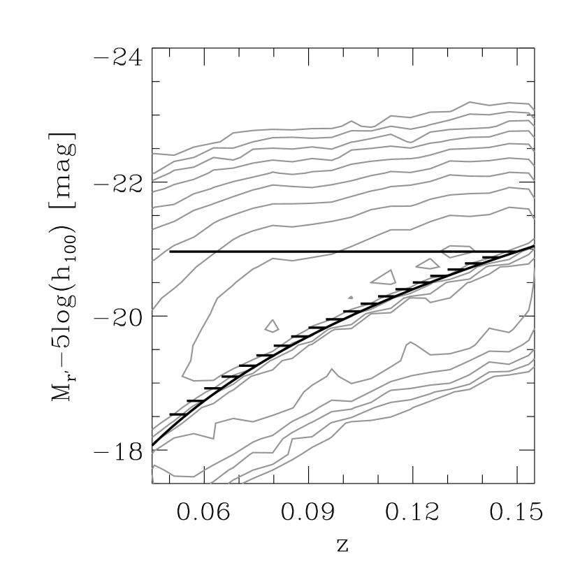
Figure 1.— The absolute Petrosian magnitude distribution of all NYU Catalog galaxies from the DR6 in redshift space (gray contours). The solid curve is the completeness limit of the SDSS instrument in the $r^{\prime}$-band. The redshift dependent cuts in absolute magnitude $M_{r^{\prime}}$ in each redshift bin of the Main Galaxy (MG) sample are represented by the short solid horizontal lines of width $\vartriangle$z = 0.005. The wider solid line with $\vartriangle$z = 0.1 is the adopted $M_{r^{\prime}}$ limit of -21.0 for the Luminous Galaxy (LG) sample (see Tables 1 & 3). The median redshift of the SDSS main galaxy sample is $\sim$ 0.1.

2.2.1 MG1: Selecting with H$\alpha$

The H$\alpha$ spectral line is the most reliable tracer of ongoing star formation at optical wavelengths (Kennicutt 1998; Yan et al. 2006): star-forming galaxies have significant H$\alpha$ emission, and H$\alpha$ is not strongly affected by, $e.g.$ dust. However, there is no a priori reason why galaxies that do not have H$\alpha$ emission should have similar star formation histories, i.e. have uniformly high D4000 indices. We use H$\alpha$ to separate starforming and non-starforming galaxies and define our first Main Galaxy sample (MG1) to have galaxies with EW(H$\alpha$) $<$ 0Å (Table 2). Depending on the redshift bin, the MG1 sample can have up to $\sim 5,500$ galaxies (Table 4).

Previous studies have used both H$\alpha$ and [OII] to identify quiescent galaxies (Yan et al. 2006; Graves et al. 2009) and shown that this population forms a tight color-magnitude relation (CMR). However, [OII] can be strongly dust-extincted and is known to be an unreliable tracer of star formation (Jansen et al. 2001; Moustakas et al. 2006). Also, measurements of [OII] in galaxies at $z<0.06$ with ground-based observatories is problematic due to absorption at $\lambda<4000$Å by the Earth’s atmosphere. Our goal is to determine whether H$\alpha$ alone can identify a uniformly quiescent galaxy population.

2.2.2 MG2 & MG3: Selecting with Sérsic index & Color

The Sérsic index $n$ is used as a quantitative measure of a galaxy’s morphology and is determined by fitting the axisymmetric surface brightness profile $I(r)=A\textnormal{ exp}\left[-(r/r_{0})^{1/n}\right]$ to a galaxy’s surface brightness profile (Sérsic 1968). Galaxies with high Sérsic indices ($n>$ 2) tend to be bulge-dominated (early-type) systems and those with lower indices ($n<$ 2) to be disk-dominated (late-type) systems. However, while Sérsic index is a useful measure of galaxy morphology (Sérsic 1968; Cassata et al. 2005; Driver et al. 2006; van der Wel 2008), morphology alone is not a reliable tracer of ongoing star formation ($e.g.$ Schawinski et al. 2009). Also, the Sérsic index $n$ depends strongly on the filter because a galaxy’s surface brightness profile varies with observed wavelength.

Multiple studies use morphology and in particular Sérsic $n>2$ to identify red sequence galaxies, $e.g.$ Hogg et al. (2004). However, this does not provide a pure sample of red sequence galaxies: while the sample features a strong CMR, it also includes a large fraction of blue galaxies. For comparison to our H$\alpha$-selected (MG1) sample, we follow Hogg et al. (2004) and select galaxies using Sérsic $n>2$ for our second Main Galaxy sample (MG2; see Table 2). We use the Sérsic index measured in the $r^{\prime}$-band from the NYU VAGC because $r^{\prime}$ is the most sensitive of the SDSS filters. Due to small errors in the measurement of the local sky level, there is a bias of $\sim(-0.5)$ in the computed Sérsic index such that a Sérsic index of $n\sim 3.5$ is measured for a real de Vaucouleurs surface brightness profile (Blanton et al. 2005b, Blanton et al. 2005a). Depending on redshift bin, the MG2 sample includes up to $\sim 12,000$ galaxies (Table 5), $i.e.$ about twice the number of galaxies as in MG1.

For a more refined comparison sample, we apply an additional color selection based on the scatter in the CMR of the H$\alpha$-selected (MG1) sample: our third Main Galaxy (MG3) sample thus includes both a selection on morphology (Sérsic $n>2$) and color (Table 2). We use only galaxies with color $\Delta(g^{\prime}-r^{\prime})>(-3\sigma_{OBS})$, where $\sigma_{OBS}$ is the median absolute deviation (MAD) of the observed color scatter; because the color distribution is asymmetric, the MAD is more appropriate for measuring the color scatter. A more extensive discussion of the color selection is in §3.1.1. The MG3 sample has up to $\sim 8,000$ galaxies in a given redshift bin (Table 6).

2.3. Luminous Galaxy Sample

In our analysis, we test the results from the Main Galaxy sample by comparing them to a Luminous Galaxy (LG) sample where we include all the galaxies at 0.05 $<z\leq$ 0.15 and apply an absolute Petrosian magnitude limit of $M_{r^{\prime}}$ = -21.0 (81,323 galaxies; see Fig. 1). Because the LG sample spans a wide redshift range, we use the K-corrected rest-frame magnitudes and colors from the NYU VAGC. Applying the same selection criteria as in the Main Galaxy sample, we have LG1 (EW H$\alpha<0$), LG2 (Sérsic $n>2$), and LG3 ($n>2$ and color-cut). Table 3 lists the criteria for these three samples and how many galaxies are in each.

2.4. Color-Magnitude Relation & Color Scatter

To determine the color-magnitude (CM) relation in our Main and Luminous Galaxy samples, we fit a simple linear least-squares to the $r^{\prime}$ magnitude and $(g^{\prime}-r^{\prime})$ color from the NYU VAGC; the fit uses the associated photometric errors. So that we are not weighted by outliers, e.g. the blue cloud, we iteratively remove $3\sigma$ outliers (convergence in typically $<5$ iterations) to determine the best fit to the red sequence. We use the median absolute deviation (MAD) to characterize the color scatter about the CM relation. In the Main Galaxy (MG) samples, we use observed magnitude and color because we do not wish to introduce additional measurement error by converting to rest-frame values. However, because the Luminous Galaxy (LG) sample spans a redshift range ($0.05<z<0.15$), we use the rest-frame Petrosian values from the NYU VAGC.

The errors on the slope and intercept of the CM relation as well as on the observed color scatter are determined by bootstrapping 5000 datasets from the selected galaxy sample in a given redshift bin (Efron 1979). For each bootstrapped dataset, we measure the CM relation as outlined above. The distribution of the CM parameters from the bootstrapped datasets then give us the $1\sigma$ errors on the slope, intercept, and the observed color scatter about the CM relation.

Because the observed color scatter is a combination of statistical (intrinsic) and systematic (measurement) errors, we also find it useful to determine the intrinsic scatter for the different galaxy samples. To determine the intrinsic scatter in color, we do the following:

1. For each galaxy in the sample with magnitude $r^{\prime}$, we calculate the predicted $(g^{\prime}-r^{\prime})$ using the CM relation.

2. Deviations ($\delta$) in magnitude and color for the modeled CM values are added where the random deviation is drawn from the associated photometric errors in the NYU VAGC, i.e. $-\Delta r^{\prime}\leq\delta r^{\prime}\leq\Delta r^{\prime}$ where $\Delta r^{\prime}$ is that galaxy’s error in magnitude.

3. A new CM relation and color scatter are determined for the modeled galaxy sample; the original associated photometric errors for each galaxy are assumed in fitting the new CM relation.

We repeat this 5000 times for each galaxy sample, and the median value of the distribution for the modeled color scatter is subtracted in quadratures from the observed color scatter to obtain the intrinsic scatter. The error on the intrinsic scatter is determined by subtracting in quadratures the $1\sigma$ of the distribution for the modeled color scatter from the observed error.

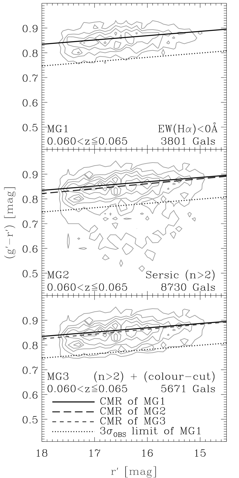
Figure 2.— The color-magnitude (CM) diagrams of MG1, MG2, and MG3 at 0.060 $<$ $z$ $\leq$ 0.065. All of the CM relations are sigma-clipped least squares fits to the plotted galaxy populations. The solid line is MG1’s (upper panel) CM relation (shown in all panels), the long-dashed line the CM relation of MG2 (middle panel), and the short-dashed line the CM relation of MG3 (bottom panel). The dotted line (shown in all panels) is the 3$\sigma_{\tiny{\textnormal{OBS}}}$ (MAD) limit of MG1’s CM relation. The number of galaxies in each subsample is indicated in the different panels.

3. Results

3.1. Main Galaxy Sample

In this section, we separate our Main Galaxy sample ($0.05<z\leq 0.15$) into galaxies with H$\alpha$ absorption (MG1), Sérsic index $n>2$ (MG2), or Sérsic index $n>2$ and red colors (MG3), and compare their physical properties. Our results are listed for the 20 redshift bins in Tables 4 to 9. However, for clarity, we focus on the galaxies in the redshift bin 0.060 $<z\leq$ 0.065 in Figures 2 to 7; this redshift bin has a large number of galaxies covering a magnitude range of about 3.5 magnitudes (see Table 1 for the MG sample).

3.1.1 MG: Color-magnitude relation

To judge which of our Main Galaxy samples has the most homogeneously red galaxy population, we compare their distribution on the color-magnitude (CM) diagram. Galaxies with uniform ages will have a narrow range in color while those with recent or ongoing star formation will populate a wide range in color (Degiola-Eastwood & Grasdalen 1980; Merluzzi et al. 2002). To ensure that we do not add to the measurement error by, e.g. converting to rest-frame magnitudes by applying k-corrections, we use apparent colors and magnitudes.

Figure 2 (top panel) shows the color distribution of the MG1 sample ($0.060<z<0.065$). We determine the CM relation with an iterative $\sigma_{\tiny{\textnormal{MAD}}}$-clipping linear least squares fit (see §2.4); because galaxy color distributions tend to be asymmetric, we use the median absolute deviation (MAD) in our analysis rather than assume a Gaussian distribution. The MG1 sample has a slope of $m=-0.017\pm 0.001$ (Table 4), and the slope stays essentially constant (approximately $m=-0.020\pm 0.003$) in all 20 redshift bins. The normalization of the CM relation increases with increasing redshift due to the stretching and shifting of the galaxy SED in the observed filters. The errors associated with fitting the CM relation also increase with redshift due to the smaller luminosity range at higher redshift (see Figure 1). This is true for all three of our Main Galaxy samples.

MG1 has an observed color scatter of only $\sigma_{\tiny{\textnormal{OBS}}}=0.0292\pm 0.0006$ (MAD value); here we measure the error for $\sigma_{\tiny{\textnormal{OBS}}}$ using the bootstrap resampling method ($e.g.$ Efron 1979; see §2.4). The color scatter is real, i.e. not dominated by noise: the intrinsic scatter is essentially identical at $\sigma_{INT}=0.0283\pm 0.0006$ (Table 4; see §2.4). Because the MG1 sample shows such a well-defined red sequence in each redshift bin, we will later use its small color scatter to exclude blue galaxies [$\Delta(g^{\prime}-r^{\prime})>-3\sigma_{\tiny{\textnormal{OBS}}}$] in MG3.

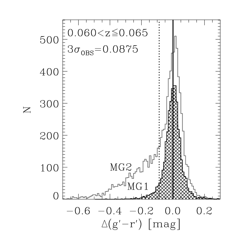
Figure 3.— Color deviation $\vartriangle$($g^{\prime}-r^{\prime}$) of MG1 (hatched distribution) and MG2 (open) in the redshift range 0.060 $<$ $z$ $\leq$ 0.065 (see Figure 2); we use the CM relation defined by MG1 to measure the color deviation for both samples. The dotted line is the 3$\sigma_{\tiny{\textnormal{OBS}}}$ (MAD) limit from MG1, and we use it to exclude bluer galaxies from the MG2 (the Sérsic sample) sample to define the MG3 sample. Note that for a Gaussian distribution, $2\sigma\sim 3\sigma_{\tiny{\textnormal{MAD}}}$.

The MG2 sample is shown in the middle panel of Figure 2 and its CM values are listed in Table 5. The CM relation for MG2 is identical to that of MG1. However, the MG2 sample has a measurably larger observed color scatter of $\sigma_{\tiny{\textnormal{OBS}}}$ = 0.0646 (MAD); this is more than twice the color scatter of MG1. MG2’s wider range in color is due to a large number of blue galaxies: about 35% of the MG2 galaxies lie below the color-cut defined by the MG1 sample (dotted line in Figure 2).

The difference in the color distribution between MG1 and MG2 are especially striking in Figure 3 which shows the color deviation $\Delta(g^{\prime}-r^{\prime})$ for both samples. MG1 has a narrow and symmetric distribution, and less than 7% of its galaxies have $\Delta(g^{\prime}-r^{\prime})<-3\sigma_{\tiny{\textnormal{OBS}}}$. In comparison, 35% of the galaxies in MG2 form an extended tail of blue galaxies.

The color distribution for our third sample, MG3, is shown in the lower panel of Figure 2 and its CM values are listed in Table 6. The CM relation in MG3 is identical to MG1 and MG2, and the observed color scatter of $\sigma_{\tiny{\textnormal{OBS}}}\sim 0.0319$ is only slightly larger than in MG1.

To summarize, the color scatter in MG2 (Sérsic $n>$ 2) is significantly higher than in MG1 and MG3; this is true in each redshift bin. From the color distributions, it is clear that MG1 selects the galaxy sample with the most uniformly red and narrowest range in color. The CM relations in the three samples are consistent with each other and with the slope of $m=-0.022$ measured by Hogg et al. (2004) using SDSS galaxies with Sérsic $n>$ 2. Because we compare the three samples in each redshift bin, our results are not affected by any bias introduced by the $3^{\prime\prime}$ fiber. The fact that the CM relation does not evolve across our redshift range also indicates that aperture bias does not affect our overall results when considering the entire redshift range ($0.05<z<0.15$).

3.1.2 MG: Fraction of Passive Galaxies

From Tables 4 - 6, we see that the fraction of galaxies in each sample varies significantly. The MG1 sample is the most restrictive: it contains only 22-37% of the galaxies in each redshift bin (see Table 4). In comparison, both the MG2 and MG3 fractions are measurably higher at 51-79% and 32-52%, respectively (Tables 5 & 6). In all three samples, the fraction increases with increasing redshift due to the higher luminosity limit, $i.e.$ only the most luminous galaxies are in the sample at higher redshift and these are predominantly passive systems (Feulner et al. 2005, 2006).

We find that almost all of the galaxies in MG1 ($>92$%) are also in MG2 and MG3, but the reverse is not true: only 43% of the galaxies in MG2 have H$\alpha$ absorption, and 62% in MG3. Although MG2 and MG3 have more galaxies than MG1, they both include emission-line (active) systems. Luminosity-weighted stacked spectra for each sample (Figure 4) confirm that MG1 does not show any measurable emission and has a high D4000 value of 1.73 while both MG2 and MG3 include active galaxies with lower D4000 values of 1.54 and 1.71, respectively. These results combined with the color analysis suggests that the H$\alpha$ absorption-line criterion may be selecting only the “core” galaxies of the red sequence.

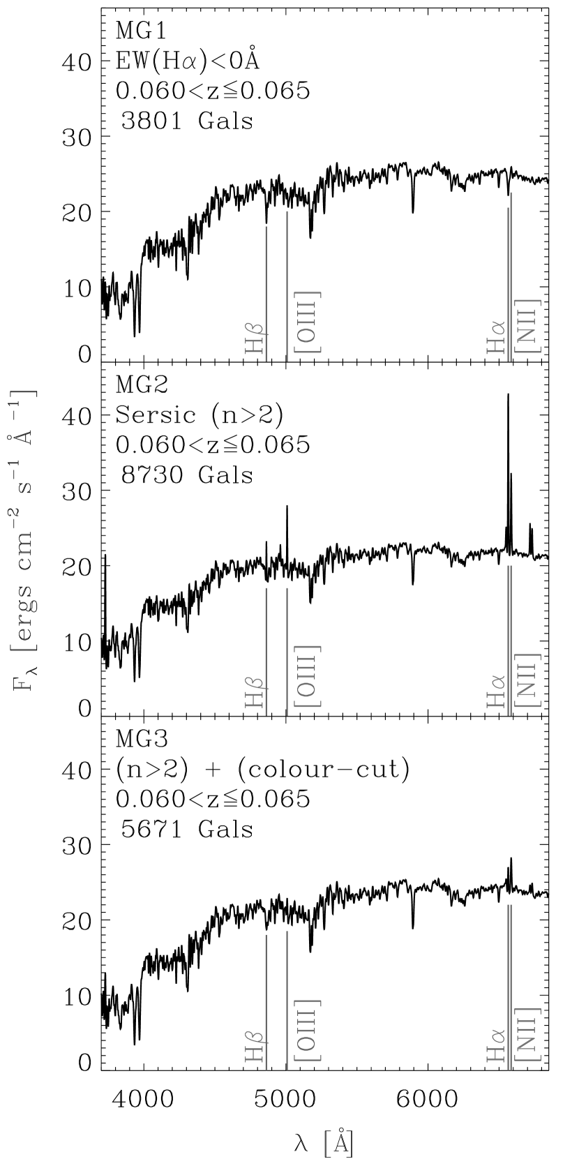
Figure 4.— Luminosity-weighted stacked spectra (rest-frame) for MG1 (top panel), MG2 (middle panel), and MG3 (bottom panel) for galaxies at $0.060<z\leq<0.065$; the spectral lines used for the BPT diagnostic are included. The stacked spectrum for MG1 shows no emission in any of the noted lines and indicates that MG1 contains the oldest galaxy population. In contrast, both MG2 and MG3 show measurable line emission in H$\alpha$.

3.1.3 MG: Star Formation vs. AGN

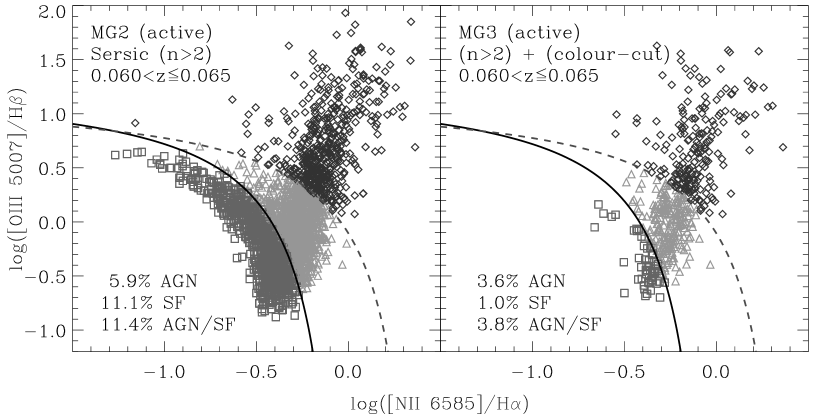
Figure 5.— The BPT-diagrams of the active galaxies in MG2 (left panel) and MG3 (right panel) in the redshift range of 0.060 $<$ $z$ $\leq$ 0.065. The black solid curve represents the separation curve of Kauffmann et al. (2003a) and the grey dotted curve the separation curve of Kewley et al. (2001). The squares represent purely star-forming (SF) galaxies, the triangles hybrid AGN/SF galaxies, and the diamonds AGN dominated galaxies; the galaxy fractions for these three categories are in the lower left corner of each panel and are calculated with respect to the total galaxy number in each sample. Applying the color-cut (MG3) reduces the fraction of active galaxies significantly, but there is still measurable contamination.

Having found that both the MG2 and MG3 samples contain active galaxies, we examine whether the activity is due to ongoing star formation or AGN. The spectral range of our stacked spectra include H$\alpha$, H$\beta$, [NII], and [OIII]; these four lines are often used to separate star-forming galaxies from those dominated by (optically-identified) AGN (Baldwin et al. 1981). Note that we only consider the MG2 and MG3 samples here because the MG1 sample, by definition, does not have any emission lines (see Fig. 4).

Figure 5 shows the BPT diagrams for the MG2 (left panel) and MG3 (right panel) samples in the redshift bin ($0.060<z\leq 0.065$). The active galaxies are separated into three categories using the curves from Kauffmann et al. (2003a) and Kewley et al. (2001): 1) star-forming; 2) AGN; and 3) combination of SF/AGN. The SF/AGN galaxies lie between the two curves and are neither clearly star-forming nor purely AGN. The fractions of galaxies in each category are calculated with respect to the total galaxy number $N_{gal}$ (see Tables 5 & 6) and are listed in Tables 7 & 8.

In our lowest redshift bin, 31% and 9% of the galaxies in the MG2 and MG3 samples, respectively, are active (Tables 7 & 8). However, the fraction of active galaxies decreases with increasing redshift because the luminosity range in the Main Galaxy samples also decreases with increasing redshift (see Figure 1). The effect is strongest in MG2 where the fraction of star-forming galaxies drops from 15% in the lowest redshift bin which has a magnitude limit of $M_{r}<-18.5$ mags to 2% in the highest redshift bin with $M_{r}<-21.0$ mags (Table 7). In comparison, the fraction of AGN in the MG2 sample only decreases from 6% to 4%, and the fraction of SF/AGN galaxies decreases by nearly half (11% to 6%). These trends indicate that the galaxies with AGN are on average brighter than those with ongoing star-formation (see also Sadler et al. 1999, 2002).

MG3 has a lower fraction of active galaxies than MG2 because the color-cut removes many of the SF and AGN/SF galaxies (Fig. 5 & Table 8). The AGN fraction in MG3 is lower than that in MG2 (3.6% vs. 6%; $0.060<z\leq 0.065$). Note that in MG3, the AGN fraction (3.6%) is measurably higher than its SF fraction (1%; Table 8). These results show that early-type ($n>2$) galaxies with AGN tend to be on the red sequence, and that most early-type galaxies with ongoing star formation are blue. As an interesting sidenote, we also find that the AGN in MG3 are not as red as the MG3 galaxies with EW(H$\alpha$)$<0$Å; like Schawinski et al. (2009), we find early-type galaxies with AGN lie closer to the “green valley”. Further study of these early-types with AGN may place useful constraints on the link between AGN and the quenching of star formation, but such an analysis is beyond the scope of this paper.

3.1.4 MG: D4000 Index & Stellar Age

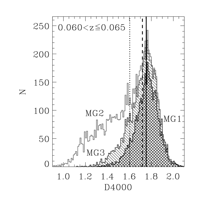
Figure 6.— The D4000 distribution of MG1 (hatched), MG2 (open), and MG3 (diagonal shaded). The average D4000 value of each sample is indicated by the solid (MG1), dashed (MG2), and dotted (MG3) lines. MG1 has the highest average D4000 value and a symmetric distribution. In contrast, MG2 and MG3 have extended tails towards lower D4000 values, i.e. they both include younger galaxies.

The D4000 index increases as a stellar population ages (Bruzual 1983; Kauffmann et al. 2003b) and can be used to compare the relative ages of the three Main Galaxy samples. Table 9 lists the median D4000 value in each redshift bin for MG1, MG2, and MG3, and Figure 6 shows how their D4000 distributions differ at ($0.060<z\leq 0.065$): MG1 has a narrow, symmetric distribution centered at D4000=1.75, but both MG2 and MG3 have asymmetric distributions with long tails extending to lower D4000 values.

In detail, more than 85% of the galaxies in MG1 have D4000$>1.60$, and none have D4000$<1.30$. In contrast, about 10% of the MG2 galaxies have D4000$<1.30$, and MG2 has a lower median D4000 value of only 1.60. In MG3, the color-cut does remove nearly all galaxies with D4000$<1.30$, but MG3’s median D4000 of 1.72 is still lower than in MG1. As a check, we also measure D4000 in the stacked spectrum for each galaxy sample (see Figure 4) and find that the values are virtually identical to our results using the D4000 distributions.

To estimate the stellar age corresponding to the median D4000 values in our three samples, we use the stellar synthesis model from Bruzual & Charlot (2003). For simplicity, we assume:

• solar metallicity (Z = 0.02)

• Salpeter initial mass function (IMF)

• single instantaneous starburst

Because we are only interested in knowing the relative age differences between the samples, we use a single metallicity and simple starburst model. The stellar ages corresponding to the median D4000 value in MG1, MG2, and MG3 are listed in Table 9. As a check, we also estimate the ages from the stacked spectrum for each sample and find that the ages measured by the two methods are consistent.

The high median D4000 value and small scatter of the H$\alpha$ selected galaxies (MG1) means that these galaxies have highly uniform and relatively old ages. The difference between MG1 and MG2 (Sérsic $n>2$) is striking: the median age in MG1 is about double that in MG2. In comparison, the red early-type sample (MG3) has a median age closer to, but never as old as, the MG1 sample (Tables 9). Note that the median age in all three samples increases with increasing redshift due to the brighter magnitude limit, $i.e.$ more luminous galaxies have older stellar populations and higher D4000 values (Gallazzi et al. 2006).

3.1.5 MG: Sérsic index vs. D4000

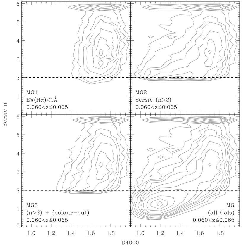
Figure 7.— The distribution of Sérsic index $n$ versus D4000 for MG1 (upper left), MG2 (upper right), MG3 (bottom left), and all galaxies (bottom right); all distributions are for the same redshift range. The dashed line inside each panel represents the Sérsic index cut-off of $n$ = 2 used to select MG2 and MG3. The overdensity at Sérsic n $\sim$ 6 is based on the NYU catalog’s imposed threshold where every galaxy with n $>$ 6 has a listed Sérsic index of $n$ = 6. MG1 (the H$\alpha$ sample) consists nearly exclusively of bulge dominated galaxies with a Sérsic index $n>$ 2.

Morphology, as quantified by the Sérsic index, is often used to identify passive galaxies because they also tend to be early-type systems ($n>2$, $e.g.$ Hogg et al. 2004). We test this assumption by comparing D4000, a robust tracer of stellar age, to the Sérsic indices from the NYU VAGC. In Figure 7 (bottom right), we plot D4000 versus Sérsic index for all the galaxies at 0.06 $<z\leq$ 0.065 in the Main Galaxy sample; the overdensity at $n=6$ is due to the NYU VAGC assigning a value of $n=6$ for any galaxy with a measured Sérsic index greater than 6.

The distribution for all galaxies is bimodal with a concentration at low D4000 ($<1.4$) and low $n$ ($<2$), and another at high D4000 ($>1.6$) and high $n$ ($>2$). Note that the color-magnitude diagram has a similar bimodal distribution (Baldry et al. 2004b). However, the correlation between Sérsic index and D4000 is quite broad, $e.g.$ a galaxy with $n=2$ can have a D4000 value from 1.0 to 1.8.

In comparison, the Sérsic and D4000 distribution of the MG1 (H$\alpha$) sample is strikingly narrow (Figure 7, top left). Even though we did not select on morphology, virtually all of the MG1 galaxies have $n>2$. As noted earlier, their D4000 distribution includes only values $>1.4$.

In MG2 and MG3 where we do select using morphology ($n>2$), the D4000 distribution is visibly broader than in MG1 (Figure 7). The contamination by younger galaxies (D4000$<1.4$) is particularly severe in the MG2 sample (top right). Applying the color-cut in the MG3 sample does remove the galaxies with D4000$<1.3$ (bottom left panel), but MG3 still contains a number of galaxies with $1.3<$D4000$<1.4$.

3.2. Luminous Galaxy Sample

Thus far we have only used the Main Galaxy sample which is divided into 20 redshift bins where the magnitude limit increases with redshift to ensure a complete sample in each redshift bin. To test the robustness of our results, we now apply an absolute magnitude limit of $M_{r^{\prime}}\leq-21.0$ set by our highest redshift bin to the entire galaxy sample ($0.05<z\leq 0.15$); this leaves us with $\sim 82,000$ galaxies (see Table 1). We divide the Luminous Galaxy sample into the same three categories as defined in Table 3: LG1 (H$\alpha$ EW$<0$Å); LG2 (Sérsic $n>2$); and LG3 (Sérsic $n>2$ and color-cut). We repeat our analysis with the Luminous Galaxy sample and compare to our results from the Main Galaxy sample. Note that because of the larger redshift range, we now use absolute rest-frame magnitudes and colors from the NYU VAGC.

3.2.1 LG: Color-Magnitude Relation

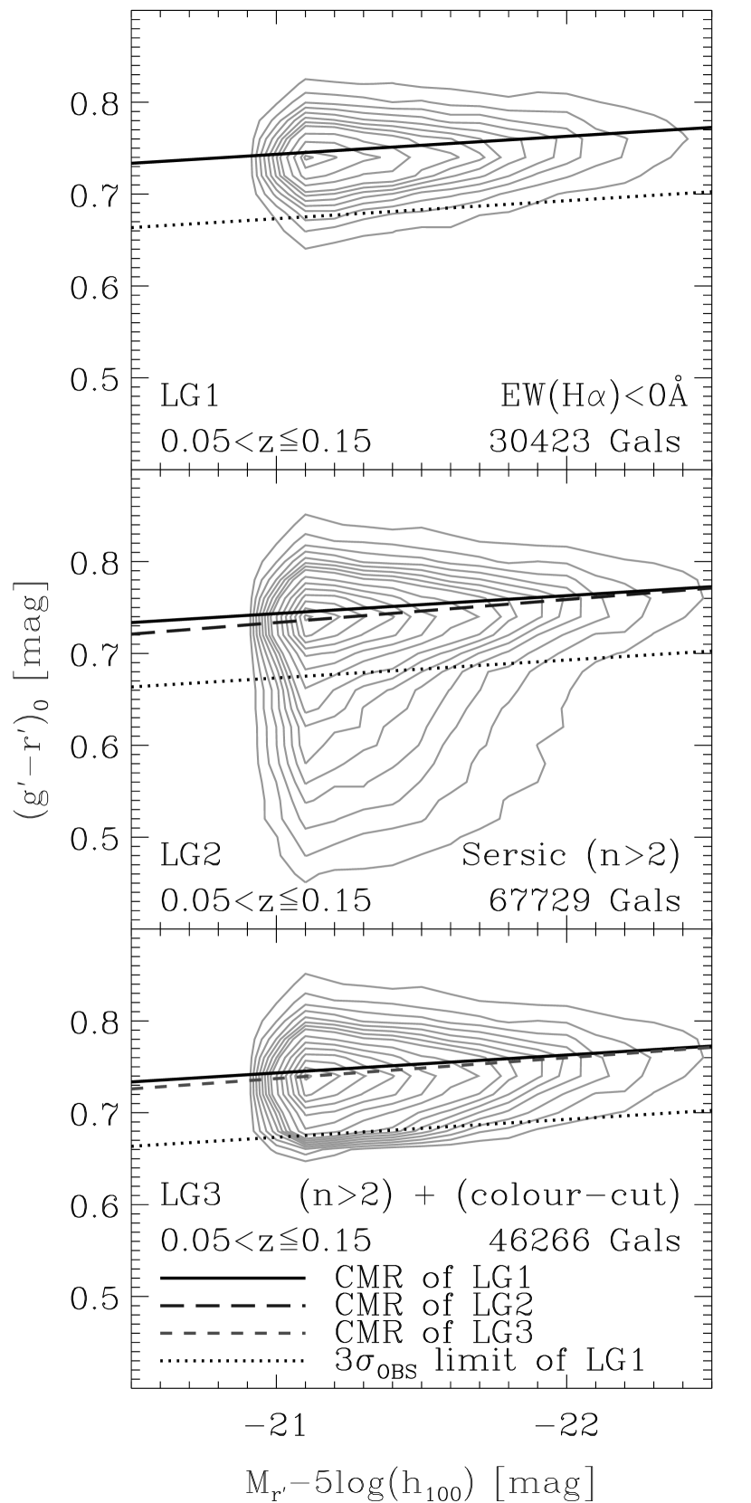
Figure 8.— Rest-frame color-magnitude diagrams for LG1 (H$\alpha$ passive; top panel), LG2 (Sérsic $n>$ 2; middle panel), and LG3 (Sérsic $n>$ 2 and color-cut; bottom panel). We consider all galaxies at $0.05<z\leq 0.15$ with $M_{r^{\prime}}$ $<$ -21.0 (see Fig. 1). The solid line is the sigma-clipped least-squares fit to LG1 (shown in all panels), the long-dashed line the fit to LG2, and the short-dashed line to LG3. The dotted line shown in all three panels represents the 3$\sigma_{\tiny{\textnormal{OBS}}}$ (MAD) limit from LG1 (3$\sigma_{\tiny{\textnormal{OBS}}}$ = 0.0700). Because of K-corrections, plotting the three galaxy samples in the rest-frame results in a tighter red sequence than plotting the samples in the observed frame (see Figure 2). However, the H$\alpha$-criterion (LG1) still isolates the most uniformly red (old) galaxy population.

The color-magnitude diagrams for LG1, LG2, and LG3 are shown in Figure 8, and their fitted color-magnitude relations are listed in Table 10. As in our earlier analysis, we use $3\sigma_{OBS}$ measured in LG1 for the color-cut applied in LG3. The CM relations for all three samples are virtually identical to each other as well as to the Main Galaxy sample; note that the normalizations are different between the Main and Luminous Galaxy samples due to the change from apparent to absolute magnitudes.

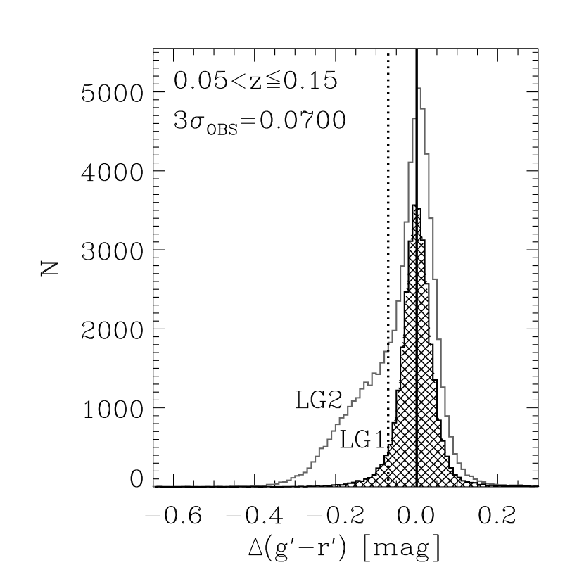
Figure 9.— Histograms of the rest-frame color residuals $\vartriangle$($g^{\prime}-r^{\prime}$) of LG1 (hatched) and LG2 (open); we use the CM relation from LG1 for both samples. The dashed line is the 3$\sigma_{\tiny{\textnormal{OBS}}}$ (MAD) of the LG1 sample used with $n>2$ to define the LG3 sample. LG1 has a very peaked and symmetric color distribution while LG2 has an extended tail towards bluer (younger) galaxies.

The observed color scatter is lowest in LG1 ($\sigma_{\tiny{\textnormal{OBS}}}$=0.023) while the scatter is twice as large in LG2 ($\sigma_{\tiny{\textnormal{OBS}}}$=0.046). LG1 has a narrow and symmetric color distribution, but LG2’s color deviation is again clearly asymmetric with a tail of bluer galaxies (see Figure 9). The color-cut in LG3 does reduce the color scatter considerably to $\sigma_{\tiny{\textnormal{OBS}}}$=0.025, but LG3 still contains a significant number of red active galaxies (see Figure 11, right panel). Note that the color scatter in the Luminous Galaxy samples are smaller than those in the Main Galaxy samples due to the higher luminosity limit and the use of rest-frame colors.

The same is true when comparing the intrinsic color scatter of LG1, LG2, and LG3 (Table 3): the LG1 sample has the lowest intrinsic color scatter. To determine the intrinsic color scatter, we correct the observed color scatter using the photometric errors listed in the NYU VAGC (see §2.4). In all cases, the color scatter is primarily due to intrinsic variations in the galaxy population and not to systematic errors.

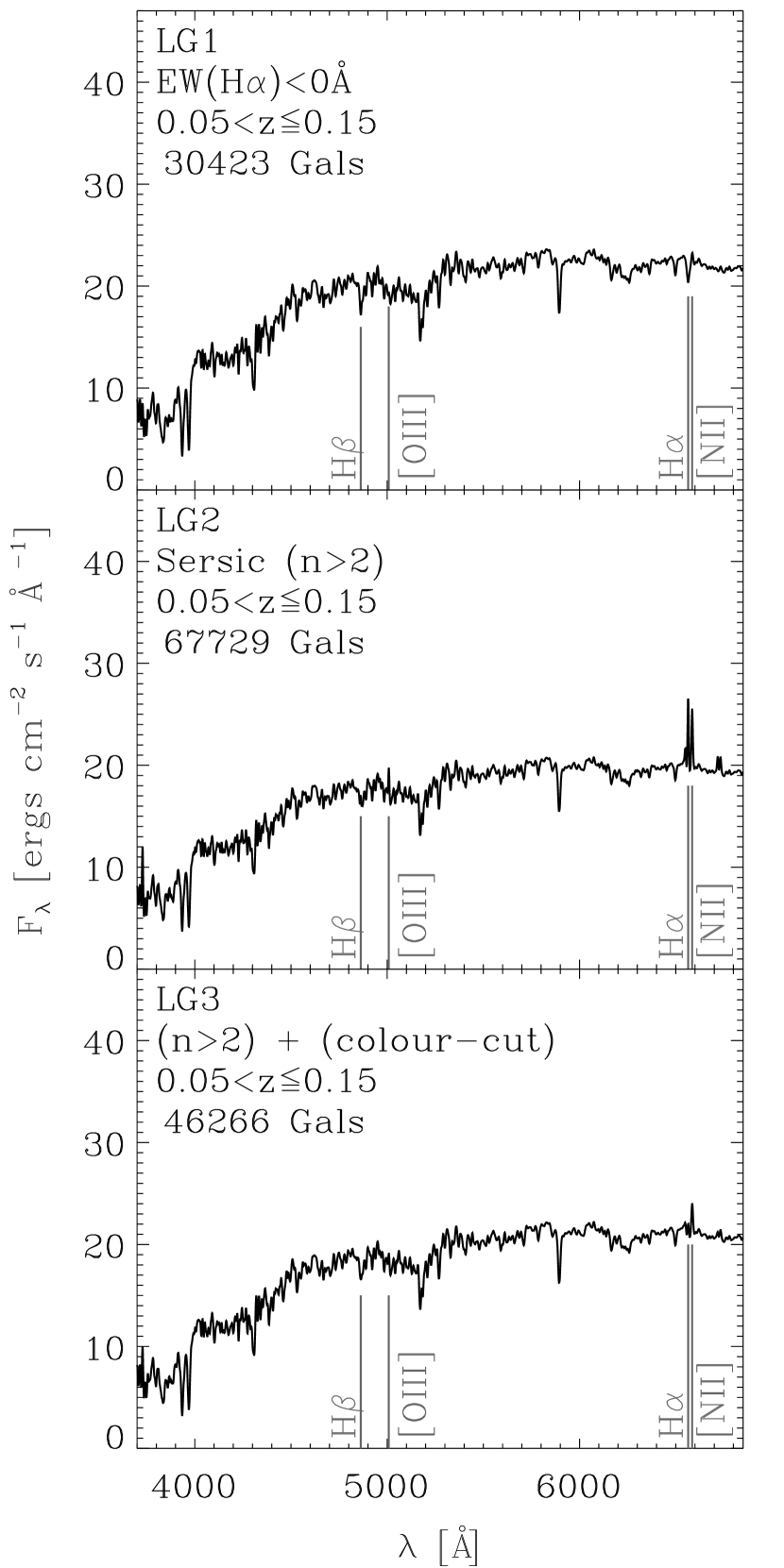
Figure 10.— Luminosity-weighted stacked spectra of LG1 (top panel), LG2 (mid panel), and LG3 (bottom panel). While the H$\alpha$ emission in LG2 and LG3 are weaker than in the Main Galaxy samples, only LG1 shows no emission in any of the noted lines. Thus even in the Luminous Galaxy samples, selecting by H$\alpha$ is still the most effective criteria for identifying a homogeneously old population.

As in the Main Galaxy sample, LG1 (H$\alpha$-selected) has the fewest galaxies while LG2 (morphology-selected) has the most (37% vs. 83%), and LG3 is in between (57%). However, the fraction of passive galaxies in LG2 and LG3 are only 44% and 62% respectively, $i.e.$ both LG2 and LG3 have a significant number of emission-line galaxies. The average luminosity-weighted stacked spectra for LG1, LG2 and LG3 confirm that L1 is composed of completely passive galaxies (Figure 10) while both LG2 and LG3 include active systems; the nearly equal emission strength in H$\alpha$ and [NII] indicate that the active galaxies in LG2 and LG3 are mostly AGN. As noted earlier, the predominance of AGN rather than ongoing star formation is due to the brighter luminosity limit ($M_{r^{\prime}}<-21.0$) in the Luminous Galaxy sample: the fainter galaxies that are excluded tend to be star-forming systems while the more luminous galaxies tend to have AGN ($e.g.$ see Table 7).

3.2.2 LG: Star Formation vs. AGN

We use the BPT diagram again to separate purely star-forming galaxies from those with AGN; this is only possible with the LG2 and LG3 samples because they both have galaxies with emission lines while the LG1 sample does not (Figure 11). Of the galaxies in LG2, 14% are active systems. The active fraction is lower in LG3 at only 3%. In both LG2 and LG3, the majority of the active galaxies have AGN. This reinforces our earlier results showing that the bright active galaxies tend to have AGN rather than ongoing star formation ($e.g.$ see Tables 7 - 8).

3.2.3 LG: D4000 Index & Stellar Age

The D4000 distributions of LG1, LG2, and LG3 are shown in Figure 12: the LG1 sample has the narrowest and most symmetric D4000 distribution, and it has the highest mean value of 1.80. The LG2 sample has the widest D4000 distribution with an asymmetric tail towards lower values; its mean value is only 1.69. Because the color-cut in LG3 tends to remove star-forming galaxies that have lower D4000 indices, its mean D4000 value is higher at 1.77. As a check, we also measure the D4000 indices in the stacked spectra (Figure 10) and find the results to be consistent.

Using the same BC03 starburst model as in §3.1.4, we determine the stellar ages as measured by the D4000 index. Because LG1 has the highest mean D4000 value, it has the oldest mean stellar age of 4.5 Gyr while LG2 has a mean age of only 3.0 Gyr. Thus even in a luminous galaxy sample, the H$\alpha$ selection continues to be the most effective criteria for isolating a uniformly quiescent galaxy population.

The Luminous Galaxy samples have higher mean D4000 indices and thus older mean stellar ages relative to the Main Galaxy samples. The Main Galaxy samples are younger due to the inclusion of fainter galaxies that tend to have more ongoing star formation. In other words, more luminous galaxies tend to have older stellar populations, as found in previous studies (Gallazzi et al. 2006; Graves et al. 2007).

3.2.4 LG: Sérsic index vs. D4000

Finally, we compare how well Sérsic index correlates with D4000 in the Luminous Galaxy samples. The results for the Luminous Galaxy samples (Figure 13) are essentially the same as in the Main Galaxy samples (Figure 7): When considering the entire Luminous Galaxy sample, the distribution is bimodal. However, the H$\alpha$ selection (LG1) contains only galaxies with $n>2$ and D4000$>1.5$. Both of the morphologically-selected samples (LG2 & LG3) have wider distributions.

In summary, we confirm that using only H$\alpha$ is as effective in the Luminous Galaxy sample as in the Main Galaxy sample at isolating a galaxy population that is highly uniform in color (red), D4000 index (high), and morphology ($n>2$).

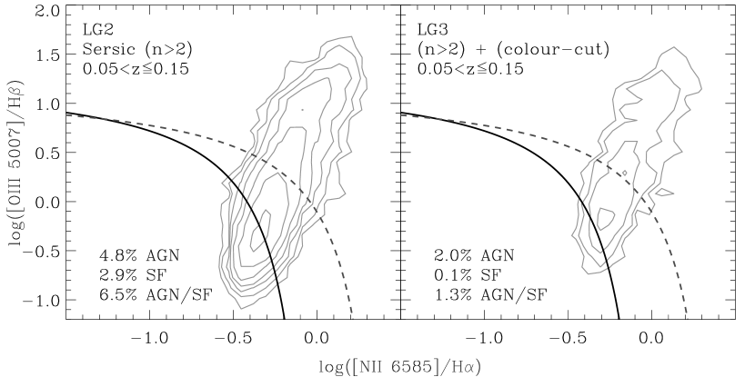
Figure 11.— The BPT-diagrams of the active galaxies in LG2 (left panel; 14.2% of all LG2 galaxies) and LG3 (right panel; 3.4% of all LG3 galaxies). The solid curve represents the separation curve of Kauffmann et al. (2003a) and the dotted curve the separation curve of Kewley et al. (2001). The relative fraction of active galaxies in the Luminous Galaxy samples is lower than in the Main Galaxy samples (Figure 5) due to the higher luminosity limit of the LG samples. However, both LG2 and LG3 still have measurable contributions from SF/AGN galaxies.

4. Discussion

The properties of the oldest galaxies at any redshift provide strong constraints on both galaxy formation models (Bower et al. 2006; Font et al. 2008) and cosmological parameters, $e.g.$ how the Hubble parameter evolves with redshift (Stern et al. 2009). Specifically, the observed color distribution of a uniformly aged population is a straight-forward test of galaxy formation models, and stellar population models must be able to reproduce the observed age distribution and remain consistent with the universe’s age at any redshift. However, how to identify a galaxy population with such homogeneous mean stellar ages continues to be debated because of mixed success using morphologically and/or color-selected samples: these selection techniques are unable to exclude a number of galaxies with ongoing star formation, particularly at $L<L^{\ast}$ (Yan et al. 2006).

Given the importance of identifying a uniformly old galaxy population, especially at higher redshift, we have introduced a new method that relies solely on the H$\alpha$ line. We find that galaxies with EW(H$\alpha)<0$Å have a narrow and symmetric color distribution (Figs. 2 & 3) with an observed color scatter of $\sigma_{\tiny{\textnormal{OBS}}}(g^{\prime}-r^{\prime})=0.029$ (MAD) in our lowest redshift bin ($z\sim 0.05$) and 0.038 in our highest redshift bin ($z\sim 0.15$). When we remove systematic errors to obtain the intrinsic color scatter, we find that the observed color scatter is dominated by real variations in the galaxy population with $\sigma_{\tiny{\textnormal{INT}}}=0.0287$ ($z\sim 0.05$) to $\sigma_{\tiny{\textnormal{INT}}}=0.0357$ ($z\sim 0.15$); these values are for photometry in the observed frame, i.e. without K-corrections.

The slope in the color-magnitude relation of $m=-0.02$ is constant throughout our 20 redshift bins (Table 4). Our results do not change even when considering only the most luminous ($M_{r^{\prime}}<-21.0$) galaxies across the entire redshift range (Figs. 8 & 9): the slope in the CM relation is the same, and the absolute color scatter is $\sigma_{\tiny{\textnormal{OBS}}}(g^{\prime}-r^{\prime})=0.023$. We also find that all of the H$\alpha$ selected galaxies have morphological Sérsic indices of $n\geqslant 2$, $i.e.$ they are all bulge-dominated systems (Sérsic 1968; Driver et al. 2006; van der Wel 2008).

As a check of the H$\alpha$ selected samples, we determine the average luminosity-weighted spectrum in each redshift bin for the Main and Luminous Galaxy samples (Figs. 4 & 10). The stacked spectra have no emission lines and D4000, a measure of the continuum break at 4000Å, increases from 1.72 at $z\sim 0.05$ to 1.80 at $z\sim 0.15$ (Table 9). Using a BC03 single starburst model (solar metallicity), the corresponding mean stellar ages of the H$\alpha$-selected sample is 3 to 4.25 Gyr. Note that the D4000 distributions of the H$\alpha$ selected samples are narrow and symmetric, and all of the galaxies have D4000$>1.3$ (Figs. 6 & 12).

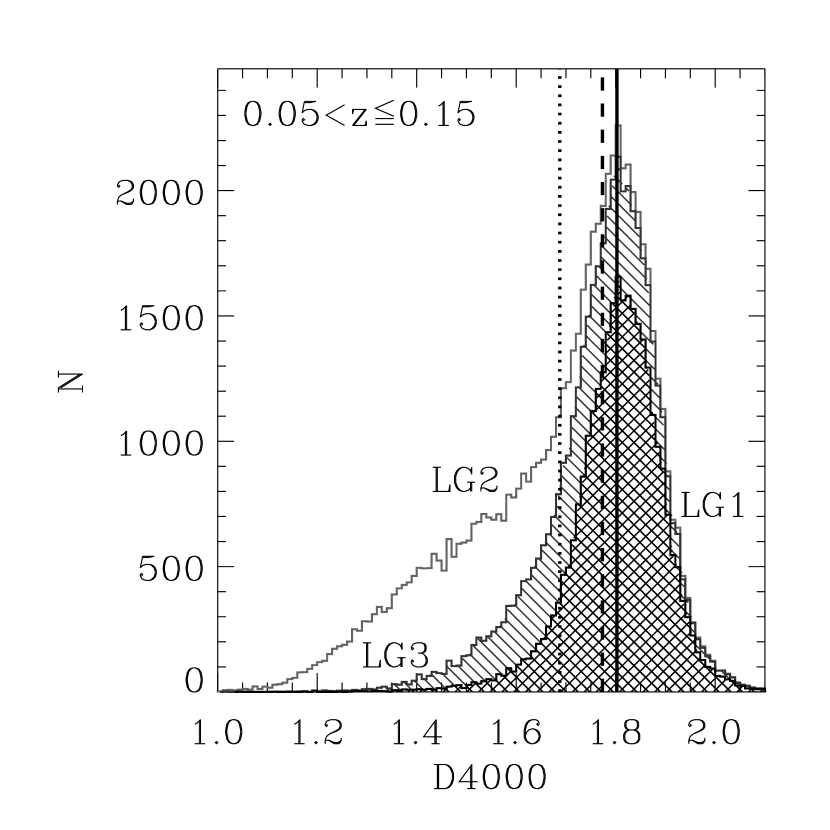
Figure 12.— The D4000 distribution of LG1 (hatched), LG2 (open), and LG3 (diagonal shaded). The average D4000 value for each sample is indicated by the solid (LG1), dashed (LG2), and dotted (LG3) lines. As in the Main Galaxy samples, LG1 has the highest average D4000 value and a symmetric distribution while both LG2 and LG3 have extended tails towards lower D4000 values, i.e. they both include younger galaxies.

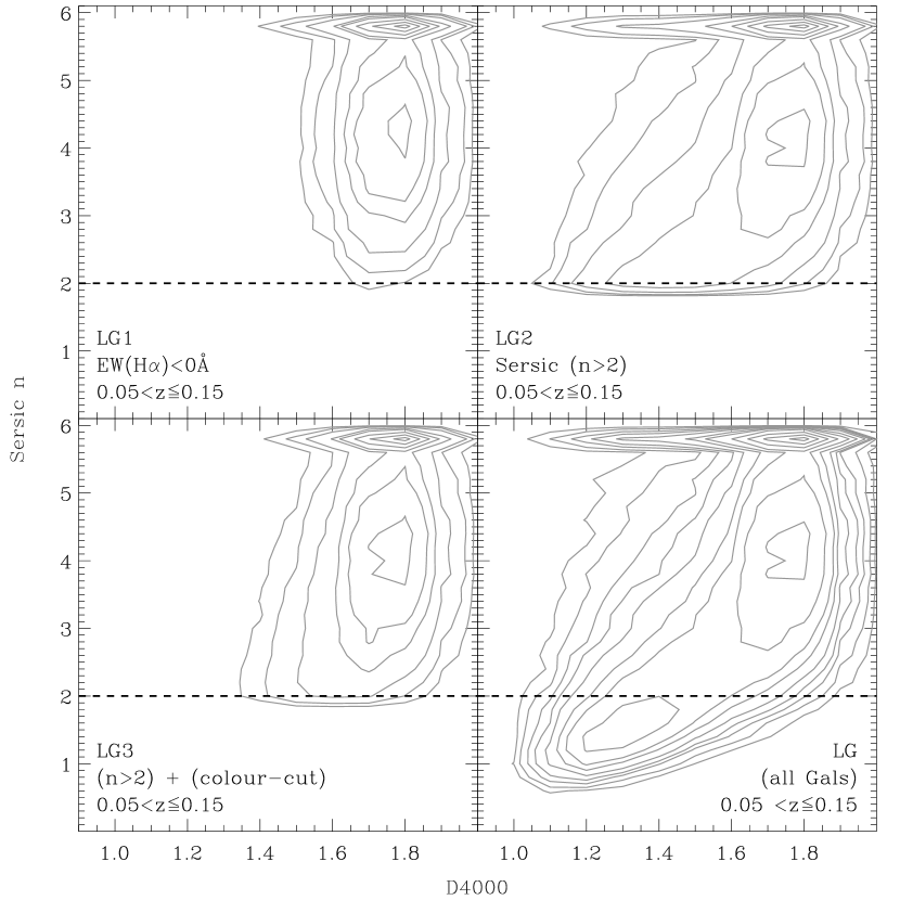
Figure 13.— The distribution of Sérsic index $n$ versus D4000 for LG1 (upper left panel), LG2 (upper right), LG3 (lower left), and all galaxies (bottom right). As in the Main Galaxy samples, the H$\alpha$-selected Luminous Galaxy sample (LG1) consists nearly exclusively of bulge-dominated galaxies ($n\geq 2$) and high D4000 values.

We quantify the effectiveness of our H$\alpha$-selection by comparing to both morphologically and color-selected samples. Following Hogg et al. (2004), we select galaxies with early-type morphologies by using Sérsic $n>2$. We find that while the slope of the CM relation is the same as in the H$\alpha$-selected samples, the distribution in both color and D4000 index is significantly wider with asymmetric tails towards bluer galaxies with lower D4000 indices (Figs. 2, 3, 6, & 7). About 35% of the ($n>2$) galaxies have $\Delta(g^{\prime}-r^{\prime})<-3\sigma_{\tiny{\textnormal{OBS}}}$ (where $\sigma_{\tiny{\textnormal{OBS}}}$ defined by the H$\alpha$ samples), and their observed color scatter is twice that of the H$\alpha$-selected samples (Tables 5 & 6).

The morphologically-selected samples have a significant fraction of active galaxies, and their stacked spectra have strong emission lines (Figs. 4 & 5). Due to the increasing magnitude limit in the redshift bins, the active fraction decreases from 32% at $z\sim 0.05$ to 13% at $z\sim 0.15$ (Table 7 & 8). The relative fraction of galaxies with ongoing star formation versus those with AGN also depends on the luminosity limit: active galaxies that are fainter than $M_{r^{\prime}}=-20.0$ tend to be dominated by star formation instead of AGN. Because of these star-forming systems, the ($n>2$) samples have lower mean D4000 indices of 1.51–1.69 ($0.05<z\leq 0.15$; Table 9); the corresponding stellar ages (1.20 to 3.00 Gyr) are about half that of the H$\alpha$-selected samples (Table 9).

Having established that the H$\alpha$-selected sample is more homogeneous in age than the morphologically-selected sample, we also test if applying a color-cut to the $n>2$ sample eliminates the emission-line galaxies. Using the observed color scatter $\sigma_{\tiny{\textnormal{OBS}}}$ determined from the H$\alpha$ samples, we exclude all $n>2$ galaxies that are bluer than $3\sigma_{\tiny{\textnormal{OBS}}}$. We find that while the color-cut does reduce the active fraction considerably, the galaxy sample is still not as uniform in color and D4000 (stellar age) as the H$\alpha$ samples (Figs. 2, 3, & 6; Table 9).

We find that our single selection criterion of EW(H$\alpha)<0$Å is more effective than using Sérsic index and/or color cuts to identify a galaxy population that is homogeneous in color (red), D4000 index (high), and morphology ($n>2$). This is true in both our Main Galaxy sample where we use a varying magnitude limit that depends on redshift, and in the Luminous Galaxy sample where we apply an absolute magnitude limit of $M_{r^{\prime}}<-21.0$. Note that even in the LGS where the galaxies are dominated by older stellar populations, there is still measurable contamination from active systems when selecting by Sérsic index and/or color.

Our ability to measure H$\alpha$ emission is not as strongly dependent on redshift as measuring Sérsic index: while quantifying galaxy morphology at $z>0.5$ requires imaging resolution of $<0.1^{\prime\prime}$, identifying galaxies with EW(H$\alpha$)$<0$Å can be done with even low signal-to-noise ($<2$) spectra. The main limitation of using H$\alpha$ is that the spectral line moves into the infrared for galaxies at $z>0.4$. However, the recent development of multi-object infrared spectrographs enables us to select with H$\alpha$ to $z\sim 2$.

5. Conclusion

By combining the SDSS DR6 with the NYU VAGC, we obtain a sample of over 180,000 galaxies at $0.05<z<0.15$ with $u^{\prime}g^{\prime}r^{\prime}i^{\prime}z^{\prime}$ photometry, Sérsic index, and measured spectral indices (Main Galaxy sample; MG). In an effort to find the most effective observational method of identifying a truly quiescent red sequence, we select galaxies solely by their H$\alpha$ line. We compare the galaxies with H$\alpha$ equivalent widths of $<0$Å, $i.e.$ in absorption, to galaxy samples selected using the more common methods of morphology (Sérsic index) and color. Our work complements earlier studies (Gallazzi et al. 2006; Graves et al. 2009) by rigorously testing which selection criteria identifies the most homogeneously aged red sequence.

We split the Main Galaxy sample into 20 redshift bins that have an increasing luminosity limit with redshift; this ensures that we are complete in each magnitude bin ($\Delta z=0.005$) and, by comparing the samples within each redshift bin, we also minimize any bias due to the $3^{\prime\prime}$ fiber aperture. We repeat our analysis using a Luminous Galaxy (LG) sample where we apply an absolute magnitude limit of $M_{r^{\prime}}<-21.0$ over the entire redshift range.

We measure the slope of the color-magnitude relation to be $m=-0.02$ which is consistent with the slope determined by Hogg et al. (2004). The slope stays constant throughout our analysis, $i.e.$ the slope does not depend on galaxy selection method nor redshift bin. However, the galaxies with EW(H$\alpha$)$<0$Å have the narrowest and most symmetric distributions in color and D4000 index, and their stacked spectra show no sign of emission lines. Also, all of the H$\alpha$ selected galaxies have Sérsic $n\geqslant 2$, $i.e.$ they are all bulge-dominated systems.

In comparison, the early-type (Sérsic $n>2$) samples include a significant number of blue/star-forming galaxies and have a color scatter that is twice as large as in the H$\alpha$ sample, $e.g.$ observed $\sigma_{\tiny{\textnormal{MAD}}}(g^{\prime}-r^{\prime})=0.077$ vs. 0.038 at $z\sim 0.15$. Their stacked spectra also show strong emission lines. Using D4000 to estimate mean stellar age, we find that the average $n>2$ galaxy is only two-thirds as old as the average H$\alpha$-selected galaxy, $e.g.$ 3.0 vs. 4.5 Gyr at $z\sim 0.15$.

Applying a color-cut to the morphologically-selected sample does reduce the fraction of star-forming galaxies. However, the color and D4000 distributions are still wider and more asymmetric than in the H$\alpha$ sample, $i.e.$ the sample still contains active galaxies. From the spectral line ratios, we find that the early-type galaxies with emission lines tend to have AGN rather than ongoing star formation.

Our analysis confirms that selecting galaxies with EW(H$\alpha$)$<0$Å is the most effective method for identifying an extremely pure, homogeneously aged galaxy population. Note that with the development of near-infrared spectrographs, H$\alpha$ can be measured to $z\sim 2$ whereas an imaging resolution of $<0.1^{\prime\prime}$ is needed to quantify galaxy morphology at $z>0.5$. By isolating the truly quiescent galaxies that populate and stay on the red sequence as a function of redshift, we are better able to quantify how their number density and masses evolve.

Table 1Main Galaxy (MG) Sample

$\vartriangle$z	$N_{gal}$	$M_{r^{\prime}}$
0.050 $<z\leq$ 0.055	13,167	-18.5
0.055 $<z\leq$ 0.060	12,283	-18.7
0.060 $<z\leq$ 0.065	15,959	-18.9
0.065 $<z\leq$ 0.070	16,207	-19.1
0.070 $<z\leq$ 0.075	18,820	-19.3
0.075 $<z\leq$ 0.080	19,408	-19.4
0.080 $<z\leq$ 0.085	19,675	-19.6
0.085 $<z\leq$ 0.090	16,721	-19.7
0.090 $<z\leq$ 0.095	14,296	-19.8
0.095 $<z\leq$ 0.100	14,094	-20.0
0.100 $<z\leq$ 0.105	13,324	-20.1
0.105 $<z\leq$ 0.110	13,210	-20.2
0.110 $<z\leq$ 0.115	14,172	-20.3
0.115 $<z\leq$ 0.120	13,193	-20.4
0.120 $<z\leq$ 0.125	11,580	-20.5
0.125 $<z\leq$ 0.130	11,807	-20.6
0.130 $<z\leq$ 0.135	11,974	-20.7
0.135 $<z\leq$ 0.140	10,736	-20.8
0.140 $<z\leq$ 0.145	9,264	-20.9
0.145 $<z\leq$ 0.150	8,641	-21.0

Table 2Selection Criteria for Main Galaxy (MG) Sample

Sample	Selection	EW H$\alpha$	Sérsic $n$	color-cut
		[Å]
MG1	H$\alpha$	$<$ 0	$\cdots$	$\cdots$
MG2	Sérsic	$\cdots$	$>$ 2	$\cdots$
MG3	Sérsic + color-cut	$\cdots$	$>$ 2	3$\sigma_{\tiny{\textnormal{OBS}}}$ of CMR

Table 3Selection Criteria for Luminous Galaxy (LG) Sample

Sample	Selection	EW H$\alpha$	Sérsic $n$	color-cut	$N_{gal}$
		[Å]
LG1	H$\alpha$	$<$ 0	$\cdots$	$\cdots$	30,423
LG2	Sérsic	$\cdots$	$>$ 2	$\cdots$	67,729
LG3	Sérsic + color-cut	$\cdots$	$>$ 2	3$\sigma_{\tiny{\textnormal{OBS}}}$ of CMR	46,266

Table 4Color-magnitude relation: MG1

$\vartriangle$z	f ($N_{gal}$)	$m$ $\pm\sigma_{m}$	$n$ $\pm\sigma_{n}$	$\sigma_{\tiny{\textnormal{OBS}}}$($g^{\prime}-r^{\prime}$)	$\sigma_{\tiny{\textnormal{INT}}}$($g^{\prime}-r^{\prime}$)
0.050 $<z\leq$ 0.055	22.5% (2,963)	-0.017 $\pm$0.001	1.12 $\pm$0.02	0.0295 $\pm$0.0007	0.0287 $\pm$0.0007
0.055 $<z\leq$ 0.060	23.4% (2,879)	-0.016 $\pm$0.002	1.12 $\pm$0.03	0.0298 $\pm$0.0008	0.0289 $\pm$0.0008
0.060 $<z\leq$ 0.065	23.8% (3,801)	-0.017 $\pm$0.001	1.15 $\pm$0.02	0.0292 $\pm$0.0006	0.0283 $\pm$0.0006
0.065 $<z\leq$ 0.070	25.4% (4,113)	-0.018 $\pm$0.001	1.17 $\pm$0.02	0.0292 $\pm$0.0006	0.0282 $\pm$0.0006
0.070 $<z\leq$ 0.075	27.5% (5,179)	-0.017 $\pm$0.001	1.17 $\pm$0.02	0.0296 $\pm$0.0005	0.0286 $\pm$0.0005
0.075 $<z\leq$ 0.080	28.0% (5,433)	-0.018 $\pm$0.001	1.20 $\pm$0.02	0.0292 $\pm$0.0005	0.0281 $\pm$0.0005
0.080 $<z\leq$ 0.085	29.5% (5,799)	-0.016 $\pm$0.001	1.18 $\pm$0.02	0.0305 $\pm$0.0005	0.0293 $\pm$0.0005
0.085 $<z\leq$ 0.090	29.5% (4,940)	-0.015 $\pm$0.002	1.17 $\pm$0.03	0.0315 $\pm$0.0005	0.0302 $\pm$0.0005
0.090 $<z\leq$ 0.095	30.0% (4,286)	-0.016 $\pm$0.002	1.21 $\pm$0.03	0.0323 $\pm$0.0006	0.0311 $\pm$0.0006
0.095 $<z\leq$ 0.100	30.0% (4,231)	-0.016 $\pm$0.002	1.22 $\pm$0.04	0.0328 $\pm$0.0007	0.0315 $\pm$0.0007
0.100 $<z\leq$ 0.105	27.8% (3,708)	-0.018 $\pm$0.002	1.27 $\pm$0.03	0.0328 $\pm$0.0007	0.0314 $\pm$0.0006
0.105 $<z\leq$ 0.110	30.0% (3,964)	-0.022 $\pm$0.002	1.34 $\pm$0.04	0.0338 $\pm$0.0007	0.0324 $\pm$0.0006
0.110 $<z\leq$ 0.115	31.4% (4,455)	-0.022 $\pm$0.003	1.36 $\pm$0.05	0.0326 $\pm$0.0006	0.0311 $\pm$0.0006
0.115 $<z\leq$ 0.120	28.8% (3,803)	-0.015 $\pm$0.003	1.26 $\pm$0.04	0.0362 $\pm$0.0007	0.0347 $\pm$0.0007
0.120 $<z\leq$ 0.125	28.7% (3,320)	-0.020 $\pm$0.003	1.37 $\pm$0.05	0.0359 $\pm$0.0009	0.0343 $\pm$0.0009
0.125 $<z\leq$ 0.130	31.6% (3,729)	-0.024 $\pm$0.003	1.44 $\pm$0.05	0.0368 $\pm$0.0007	0.0352 $\pm$0.0007
0.130 $<z\leq$ 0.135	34.5% (4,129)	-0.021 $\pm$0.003	1.41 $\pm$0.05	0.0375 $\pm$0.0008	0.0358 $\pm$0.0008
0.135 $<z\leq$ 0.140	36.2% (3,890)	-0.024 $\pm$0.003	1.47 $\pm$0.05	0.0365 $\pm$0.0008	0.0346 $\pm$0.0007
0.140 $<z\leq$ 0.145	36.8% (3,413)	-0.023 $\pm$0.003	1.48 $\pm$0.06	0.0369 $\pm$0.0009	0.0349 $\pm$0.0008
0.145 $<z\leq$ 0.150	36.7% (3,171)	-0.028 $\pm$0.004	1.58 $\pm$0.06	0.0377 $\pm$0.0009	0.0357 $\pm$0.0009

Table 5Color-magnitude relation: MG2

$\vartriangle$z	f ($N_{gal}$)	m $\pm\sigma_{m}$	n $\pm\sigma_{n}$	$\sigma_{\tiny{\textnormal{OBS}}}$($g^{\prime}-r^{\prime}$)	$\sigma_{\tiny{\textnormal{INT}}}$($g^{\prime}-r^{\prime}$)
0.050 $<z\leq$ 0.055	50.9% ( 6,703)	-0.017 $\pm$0.002	1.12 $\pm$0.04	0.0686 $\pm$0.0014	0.0682 $\pm$0.0014
0.055 $<z\leq$ 0.060	52.2% ( 6,410)	-0.017 $\pm$0.002	1.12 $\pm$0.04	0.0661 $\pm$0.0015	0.0657 $\pm$0.0015
0.060 $<z\leq$ 0.065	54.7% ( 8,730)	-0.020 $\pm$0.002	1.18 $\pm$0.04	0.0646 $\pm$0.0012	0.0642 $\pm$0.0012
0.065 $<z\leq$ 0.070	55.6% ( 9,019)	-0.019 $\pm$0.002	1.19 $\pm$0.04	0.0640 $\pm$0.0010	0.0636 $\pm$0.0010
0.070 $<z\leq$ 0.075	58.9% (11,081)	-0.017 $\pm$0.002	1.17 $\pm$0.03	0.0604 $\pm$0.0010	0.0599 $\pm$0.0010
0.075 $<z\leq$ 0.080	60.5% (11,735)	-0.017 $\pm$0.002	1.18 $\pm$0.03	0.0604 $\pm$0.0009	0.0598 $\pm$0.0008
0.080 $<z\leq$ 0.085	63.0% (12,395)	-0.018 $\pm$0.002	1.21 $\pm$0.04	0.0622 $\pm$0.0009	0.0616 $\pm$0.0009
0.085 $<z\leq$ 0.090	63.7% (10,652)	-0.017 $\pm$0.002	1.20 $\pm$0.04	0.0633 $\pm$0.0010	0.0627 $\pm$0.0010
0.090 $<z\leq$ 0.095	63.8% ( 9,119)	-0.014 $\pm$0.003	1.17 $\pm$0.05	0.0663 $\pm$0.0011	0.0657 $\pm$0.0011
0.095 $<z\leq$ 0.100	65.8% ( 9,267)	-0.018 $\pm$0.003	1.25 $\pm$0.05	0.0660 $\pm$0.0012	0.0653 $\pm$0.0012
0.100 $<z\leq$ 0.105	65.7% ( 8,755)	-0.022 $\pm$0.003	1.31 $\pm$0.05	0.0682 $\pm$0.0012	0.0675 $\pm$0.0012
0.105 $<z\leq$ 0.110	67.3% ( 8,887)	-0.023 $\pm$0.003	1.36 $\pm$0.05	0.0680 $\pm$0.0012	0.0673 $\pm$0.0012
0.110 $<z\leq$ 0.115	69.9% ( 9,906)	-0.025 $\pm$0.003	1.39 $\pm$0.05	0.0700 $\pm$0.0011	0.0692 $\pm$0.0011
0.115 $<z\leq$ 0.120	70.5% ( 9,300)	-0.024 $\pm$0.003	1.39 $\pm$0.06	0.0738 $\pm$0.0011	0.0731 $\pm$0.0011
0.120 $<z\leq$ 0.125	70.2% ( 8,124)	-0.027 $\pm$0.004	1.46 $\pm$0.06	0.0765 $\pm$0.0014	0.0757 $\pm$0.0014
0.125 $<z\leq$ 0.130	72.4% ( 8,545)	-0.029 $\pm$0.004	1.51 $\pm$0.06	0.0766 $\pm$0.0013	0.0758 $\pm$0.0013
0.130 $<z\leq$ 0.135	75.3% ( 9,013)	-0.027 $\pm$0.004	1.50 $\pm$0.06	0.0763 $\pm$0.0014	0.0755 $\pm$0.0014
0.135 $<z\leq$ 0.140	76.7% ( 8,237)	-0.029 $\pm$0.004	1.55 $\pm$0.07	0.0762 $\pm$0.0014	0.0753 $\pm$0.0014
0.140 $<z\leq$ 0.145	77.4% ( 7,169)	-0.031 $\pm$0.005	1.60 $\pm$0.08	0.0761 $\pm$0.0014	0.0752 $\pm$0.0014
0.145 $<z\leq$ 0.150	78.5% ( 6,781)	-0.039 $\pm$0.005	1.75 $\pm$0.09	0.0771 $\pm$0.0016	0.0761 $\pm$0.0016

Table 6Color-magnitude relation: MG3

$\vartriangle$z	f ($N_{gal}$)	m $\pm\sigma_{m}$	n $\pm\sigma_{n}$	$\sigma_{\tiny{\textnormal{OBS}}}$($g^{\prime}-r^{\prime}$)	$\sigma_{\tiny{\textnormal{INT}}}$($g^{\prime}-r^{\prime}$)
0.050 $<z\leq$ 0.055	32.3% (4,252)	-0.018 $\pm$0.001	1.13 $\pm$0.02	0.0321 $\pm$0.0007	0.0313 $\pm$0.0007
0.055 $<z\leq$ 0.060	33.8% (4,153)	-0.017 $\pm$0.001	1.12 $\pm$0.02	0.0323 $\pm$0.0006	0.0314 $\pm$0.0006
0.060 $<z\leq$ 0.065	35.5% (5,671)	-0.020 $\pm$0.001	1.18 $\pm$0.02	0.0319 $\pm$0.0005	0.0310 $\pm$0.0005
0.065 $<z\leq$ 0.070	36.0% (5,831)	-0.019 $\pm$0.001	1.18 $\pm$0.02	0.0312 $\pm$0.0005	0.0302 $\pm$0.0005
0.070 $<z\leq$ 0.075	39.4% (7,407)	-0.017 $\pm$0.001	1.16 $\pm$0.02	0.0313 $\pm$0.0005	0.0302 $\pm$0.0005
0.075 $<z\leq$ 0.080	39.7% (7,710)	-0.017 $\pm$0.001	1.18 $\pm$0.02	0.0301 $\pm$0.0004	0.0289 $\pm$0.0004
0.080 $<z\leq$ 0.085	42.4% (8,334)	-0.017 $\pm$0.001	1.20 $\pm$0.02	0.0324 $\pm$0.0004	0.0312 $\pm$0.0004
0.085 $<z\leq$ 0.090	43.0% (7,183)	-0.016 $\pm$0.001	1.19 $\pm$0.02	0.0332 $\pm$0.0005	0.0319 $\pm$0.0005
0.090 $<z\leq$ 0.095	42.5% (6,071)	-0.016 $\pm$0.002	1.20 $\pm$0.03	0.0342 $\pm$0.0005	0.0329 $\pm$0.0005
0.095 $<z\leq$ 0.100	44.4% (6,261)	-0.019 $\pm$0.001	1.26 $\pm$0.03	0.0353 $\pm$0.0005	0.0339 $\pm$0.0005
0.100 $<z\leq$ 0.105	43.5% (5,796)	-0.020 $\pm$0.002	1.30 $\pm$0.03	0.0351 $\pm$0.0005	0.0337 $\pm$0.0005
0.105 $<z\leq$ 0.110	45.3% (5,980)	-0.024 $\pm$0.002	1.38 $\pm$0.03	0.0364 $\pm$0.0006	0.0350 $\pm$0.0005
0.110 $<z\leq$ 0.115	45.8% (6,485)	-0.023 $\pm$0.002	1.38 $\pm$0.04	0.0346 $\pm$0.0005	0.0330 $\pm$0.0005
0.115 $<z\leq$ 0.120	46.7% (6,167)	-0.019 $\pm$0.002	1.32 $\pm$0.03	0.0392 $\pm$0.0006	0.0377 $\pm$0.0006
0.120 $<z\leq$ 0.125	46.0% (5,322)	-0.024 $\pm$0.002	1.41 $\pm$0.04	0.0396 $\pm$0.0007	0.0380 $\pm$0.0007
0.125 $<z\leq$ 0.130	47.9% (5,652)	-0.026 $\pm$0.002	1.47 $\pm$0.04	0.0391 $\pm$0.0006	0.0374 $\pm$0.0006
0.130 $<z\leq$ 0.135	50.4% (6,035)	-0.026 $\pm$0.002	1.48 $\pm$0.04	0.0401 $\pm$0.0007	0.0383 $\pm$0.0007
0.135 $<z\leq$ 0.140	50.6% (5,430)	-0.026 $\pm$0.002	1.51 $\pm$0.04	0.0387 $\pm$0.0007	0.0367 $\pm$0.0006
0.140 $<z\leq$ 0.145	51.7% (4,789)	-0.028 $\pm$0.003	1.54 $\pm$0.05	0.0398 $\pm$0.0007	0.0378 $\pm$0.0007
0.145 $<z\leq$ 0.150	52.2% (4,509)	-0.035 $\pm$0.003	1.69 $\pm$0.05	0.0400 $\pm$0.0008	0.0379 $\pm$0.0008

Table 7Active Fractions: MG2

$\vartriangle$z	f ($N_{\tiny{\textnormal{active}}}$)	f ($N_{\tiny{\textnormal{AGN}}}$)	f ($N_{\tiny{\textnormal{AGN/SF}}}$)	f ($N_{\tiny{\textnormal{SF}}}$)
0.050$<z\leq$0.055	31.5% (2,114)	5.8% (390)	11.1% ( 747)	14.6% (977)
0.055$<z\leq$0.060	29.6% (1,896)	5.7% (363)	11.4% ( 732)	12.5% (801)
0.060$<z\leq$0.065	28.4% (2,477)	5.9% (518)	11.4% ( 991)	11.1% (968)
0.065$<z\leq$0.070	26.8% (2,421)	5.3% (479)	11.2% (1,007)	10.4% (935)
0.070$<z\leq$0.075	24.4% (2,703)	5.1% (566)	10.3% (1,139)	9.0% (998)
0.075$<z\leq$0.080	22.9% (2,683)	4.9% (574)	10.2% (1,195)	7.8% (914)
0.080$<z\leq$0.085	21.9% (2,720)	5.0% (622)	10.3% (1,275)	6.6% (823)
0.085$<z\leq$0.090	20.7% (2,202)	4.4% (472)	10.1% (1,081)	6.1% (649)
0.090$<z\leq$0.095	20.4% (1,857)	4.9% (443)	9.7% ( 886)	5.8% (528)
0.095$<z\leq$0.100	20.7% (1,914)	5.8% (536)	9.8% ( 908)	5.1% (470)
0.100$<z\leq$0.105	20.5% (1,798)	5.8% (506)	9.7% ( 850)	5.0% (442)
0.105$<z\leq$0.110	19.1% (1,693)	5.3% (468)	9.0% ( 800)	4.8% (425)
0.110$<z\leq$0.115	16.0% (1,586)	5.4% (538)	7.1% ( 706)	3.5% (342)
0.115$<z\leq$0.120	17.6% (1,633)	5.1% (478)	8.4% ( 784)	4.0% (371)
0.120$<z\leq$0.125	17.6% (1,431)	5.2% (423)	8.2% ( 665)	4.2% (343)
0.125$<z\leq$0.130	17.1% (1,462)	5.1% (435)	7.9% ( 672)	4.2% (355)
0.130$<z\leq$0.135	14.9% (1,343)	4.8% (432)	7.0% ( 628)	3.1% (283)
0.135$<z\leq$0.140	14.5% (1,191)	4.5% (369)	7.1% ( 586)	2.9% (236)
0.140$<z\leq$0.145	12.9% ( 926)	4.5% (323)	6.1% ( 438)	2.3% (165)
0.145$<z\leq$0.150	12.6% ( 853)	4.3% (292)	6.2% ( 418)	2.1% (143)

Note. — MG2 only consists of galaxies that have Sérsic n $>$ 2 in the $r^{\prime}$-band. The fractions are relative to the total number of MG2 galaxies in the same redshift bin.

Table 8Active Fractions: MG3

$\vartriangle$z	f ($N_{\tiny{\textnormal{active}}}$)	f ($N_{\tiny{\textnormal{AGN}}}$)	f ($N_{\tiny{\textnormal{AGN/SF}}}$)	f ($N_{\tiny{\textnormal{SF}}}$)
0.050$<z\leq$0.055	9.3% (394)	3.6% (152)	4.4% (186)	1.3% (56)
0.055$<z\leq$0.060	9.0% (372)	3.5% (144)	4.4% (181)	1.1% (47)
0.060$<z\leq$0.065	8.4% (474)	3.6% (202)	3.8% (216)	1.0% (56)
0.065$<z\leq$0.070	7.4% (431)	3.1% (183)	3.6% (208)	0.7% (40)
0.070$<z\leq$0.075	6.2% (460)	2.5% (184)	3.1% (229)	0.6% (47)
0.075$<z\leq$0.080	5.4% (416)	2.2% (169)	2.8% (216)	0.4% (31)
0.080$<z\leq$0.085	5.5% (460)	2.2% (186)	3.0% (246)	0.3% (28)
0.085$<z\leq$0.090	5.0% (362)	2.0% (147)	2.7% (195)	0.3% (20)
0.090$<z\leq$0.095	4.8% (291)	2.2% (135)	2.2% (131)	0.4% (25)
0.095$<z\leq$0.100	4.8% (299)	2.3% (145)	2.2% (136)	0.3% (18)
0.100$<z\leq$0.105	4.5% (262)	2.5% (145)	1.8% (105)	0.2% (12)
0.105$<z\leq$0.110	4.1% (243)	2.2% (130)	1.7% (101)	0.2% (12)
0.110$<z\leq$0.115	2.9% (189)	1.9% (125)	0.9% ( 58)	0.1% ( 6)
0.115$<z\leq$0.120	3.6% (221)	2.2% (138)	1.2% ( 72)	0.2% (11)
0.120$<z\leq$0.125	3.8% (204)	2.0% (106)	1.7% ( 90)	0.2% ( 8)
0.125$<z\leq$0.130	3.1% (178)	1.7% ( 96)	1.2% ( 70)	0.2% (12)
0.130$<z\leq$0.135	2.6% (157)	1.6% ( 99)	0.8% ( 50)	0.1% ( 8)
0.135$<z\leq$0.140	2.2% (118)	1.5% ( 81)	0.7% ( 36)	0.0% ( 1)
0.140$<z\leq$0.145	1.8% ( 88)	1.4% ( 66)	0.4% ( 20)	0.0% ( 2)
0.145$<z\leq$0.150	2.7% (121)	1.8% ( 81)	0.8% ( 36)	0.1% ( 4)

Note. — MG3 only consists of galaxies that have Sérsic $n>$ 2 in the $r^{\prime}$-band and color deviation $\vartriangle(g^{\prime}-r^{\prime})>-3\sigma_{\tiny{\textnormal{OBS}}}$ (see Figure 2, middle and bottom panels). The fractions are relative to the total number of MG3 galaxies in the same redshift bin.

Table 9Ages from Median D4000: MG1, MG2, MG3

$\vartriangle$z	$\langle$D4000$\rangle_{\tiny{\textnormal{MG1}}}$	$\langle$Age$\rangle_{\tiny{\textnormal{MG1}}}$	$\langle$D4000$\rangle_{\tiny{\textnormal{MG2}}}$	$\langle$Age$\rangle_{\tiny{\textnormal{MG2}}}$	$\langle$D4000$\rangle_{\tiny{\textnormal{MG3}}}$	$\langle$Age$\rangle_{\tiny{\textnormal{MG3}}}$
		[Gyr]		[Gyr]		[Gyr]
0.050$<z\leq$0.055	1.74 $\pm$0.07	3.25 ${}^{+1.25}_{-0.50}$	1.58 $\pm$0.16	2.00 ${}^{+1.25}_{-1.30}$	1.71 $\pm$0.09	3.00 ${}^{+1.50}_{-0.60}$
0.055$<z\leq$0.060	1.75 $\pm$0.07	3.50 ${}^{+1.25}_{-0.75}$	1.60 $\pm$0.15	2.20 ${}^{+1.30}_{-1.40}$	1.71 $\pm$0.09	3.00 ${}^{+1.50}_{-0.50}$
0.060$<z\leq$0.065	1.75 $\pm$0.07	3.50 ${}^{+1.25}_{-0.75}$	1.60 $\pm$0.14	2.20 ${}^{+1.30}_{-1.30}$	1.72 $\pm$0.08	3.00 ${}^{+1.50}_{-0.40}$
0.065$<z\leq$0.070	1.75 $\pm$0.06	3.50 ${}^{+1.25}_{-0.75}$	1.61 $\pm$0.14	2.30 ${}^{+1.20}_{-1.40}$	1.72 $\pm$0.08	3.00 ${}^{+1.50}_{-0.40}$
0.070$<z\leq$0.075	1.76 $\pm$0.06	3.75 ${}^{+1.00}_{-0.75}$	1.62 $\pm$0.13	2.40 ${}^{+1.10}_{-1.40}$	1.72 $\pm$0.08	3.00 ${}^{+1.50}_{-0.40}$
0.075$<z\leq$0.080	1.76 $\pm$0.06	3.75 ${}^{+1.00}_{-0.75}$	1.63 $\pm$0.13	2.50 ${}^{+1.25}_{-1.25}$	1.73 $\pm$0.07	3.25 ${}^{+1.25}_{-0.50}$
0.080$<z\leq$0.085	1.76 $\pm$0.06	3.75 ${}^{+1.00}_{-0.75}$	1.64 $\pm$0.12	2.60 ${}^{+1.15}_{-1.20}$	1.73 $\pm$0.07	3.25 ${}^{+1.25}_{-0.50}$
0.085$<z\leq$0.090	1.77 $\pm$0.06	4.00 ${}^{+1.00}_{-1.00}$	1.64 $\pm$0.12	2.60 ${}^{+1.15}_{-1.50}$	1.74 $\pm$0.07	3.25 ${}^{+1.25}_{-0.50}$
0.090$<z\leq$0.095	1.77 $\pm$0.06	4.00 ${}^{+1.00}_{-1.00}$	1.64 $\pm$0.12	2.60 ${}^{+1.15}_{-1.50}$	1.74 $\pm$0.07	3.25 ${}^{+1.25}_{-0.50}$
0.095$<z\leq$0.100	1.77 $\pm$0.06	4.00 ${}^{+1.00}_{-1.00}$	1.64 $\pm$0.12	2.60 ${}^{+1.15}_{-1.50}$	1.74 $\pm$0.07	3.25 ${}^{+1.25}_{-0.50}$
0.100$<z\leq$0.105	1.77 $\pm$0.06	4.00 ${}^{+1.00}_{-1.00}$	1.64 $\pm$0.13	2.60 ${}^{+1.40}_{-1.20}$	1.74 $\pm$0.07	3.25 ${}^{+1.25}_{-0.50}$
0.105$<z\leq$0.110	1.77 $\pm$0.06	4.00 ${}^{+1.00}_{-1.00}$	1.64 $\pm$0.12	2.60 ${}^{+1.40}_{-1.50}$	1.74 $\pm$0.07	3.25 ${}^{+1.25}_{-0.50}$
0.110$<z\leq$0.115	1.78 $\pm$0.06	4.00 ${}^{+1.25}_{-1.00}$	1.65 $\pm$0.12	2.75 ${}^{+1.25}_{-1.15}$	1.75 $\pm$0.07	3.50 ${}^{+1.25}_{-0.75}$
0.115$<z\leq$0.120	1.78 $\pm$0.06	4.00 ${}^{+1.25}_{-1.00}$	1.65 $\pm$0.12	2.75 ${}^{+1.25}_{-1.15}$	1.75 $\pm$0.07	3.50 ${}^{+1.25}_{-0.75}$
0.120$<z\leq$0.125	1.78 $\pm$0.06	4.00 ${}^{+1.25}_{-1.00}$	1.65 $\pm$0.12	2.75 ${}^{+1.25}_{-1.15}$	1.75 $\pm$0.07	3.50 ${}^{+1.25}_{-0.75}$
0.125$<z\leq$0.130	1.78 $\pm$0.06	4.00 ${}^{+1.25}_{-1.00}$	1.66 $\pm$0.12	2.75 ${}^{+1.25}_{-1.10}$	1.76 $\pm$0.07	3.75 ${}^{+1.00}_{-0.75}$
0.130$<z\leq$0.135	1.79 $\pm$0.06	4.25 ${}^{+1.00}_{-1.00}$	1.67 $\pm$0.11	2.75 ${}^{+1.25}_{-0.85}$	1.76 $\pm$0.06	3.75 ${}^{+1.00}_{-0.75}$
0.135$<z\leq$0.140	1.79 $\pm$0.06	4.25 ${}^{+1.00}_{-1.00}$	1.68 $\pm$0.11	2.75 ${}^{+1.50}_{-0.85}$	1.77 $\pm$0.06	4.00 ${}^{+1.00}_{-1.00}$
0.140$<z\leq$0.145	1.80 $\pm$0.06	4.50 ${}^{+1.00}_{-1.00}$	1.69 $\pm$0.11	3.00 ${}^{+1.25}_{-1.00}$	1.78 $\pm$0.06	4.00 ${}^{+1.25}_{-1.00}$
0.145$<z\leq$0.150	1.80 $\pm$0.06	4.50 ${}^{+1.00}_{-1.00}$	1.69 $\pm$0.11	3.00 ${}^{+1.50}_{-1.00}$	1.79 $\pm$0.07	4.25 ${}^{+1.00}_{-1.25}$

Note. — We use the stellar synthesis model code of Bruzual & Charlot (2003) with solar metallicity (Z = 0.02), Salpeter IMF, and the Padova stellar evolution track to determine an age.

Table 10Color-magnitude relations: LG1, LG2, LG3

Galaxy sample	$\vartriangle$z	f ($N_{\textnormal{gal}}$)	m $\pm\sigma_{m}$	n $\pm\sigma_{n}$	$\sigma_{\tiny{\textnormal{OBS}}}$($g^{\prime}-r^{\prime}$)	$\sigma_{\tiny{\textnormal{INT}}}$($g^{\prime}-r^{\prime}$)
LG1	0.05$<z\leq$0.15	37.4% (30,423)	-0.019 $\pm$0.001	0.33 $\pm$0.02	0.0233 $\pm$1.7$\cdot 10^{-4}$	0.0150 $\pm$1.4$\cdot 10^{-4}$
LG2	0.05$<z\leq$0.15	83.3% (67,729)	-0.025 $\pm$0.001	0.20 $\pm$0.02	0.0464 $\pm$2.8$\cdot 10^{-4}$	0.0428 $\pm$2.7$\cdot 10^{-4}$
LG3	0.05$<z\leq$0.15	56.9% (46.266)	-0.022 $\pm$0.001	0.26 $\pm$0.02	0.0253 $\pm$1.5$\cdot 10^{-4}$	0.0176 $\pm$1.2$\cdot 10^{-4}$

References

- Adelman-McCarthy et al. (2008) Adelman-McCarthy, J. K., Agüeros, M. A., Allam, S. S., Allende Prieto, C., Anderson, K. S. J., & et al. 2008, ApJS, 175, 297
- Baldry et al. (2004a) Baldry, I. K., Balogh, M. L., Bower, R., Glazebrook, K., & Nichol, R. C. 2004a, in American Institute of Physics Conference Series, Vol. 743, The New Cosmology: Conference on Strings and Cosmology, ed. R. E. Allen, D. V. Nanopoulos, & C. N. Pope, 106–119
- Baldry et al. (2004b) Baldry, I. K., Glazebrook, K., Brinkmann, J., Ivezić, Ž., Lupton, R. H., & et al. 2004b, ApJ, 600, 681
- Baldwin et al. (1981) Baldwin, J. A., Phillips, M. M., & Terlevich, R. 1981, PASP, 93, 5
- Baum (1959) Baum, W. A. 1959, in IAU Symposium, Vol. 10, The Hertzsprung-Russell Diagram, ed. J. L. Greenstein, 23–+
- Bell et al. (2004a) Bell, E. F., McIntosh, D. H., Barden, M., Wolf, C., Caldwell, J. A. R., Rix, H.-W., & et al. 2004a, ApJ, 600, L11
- Bell et al. (2004b) Bell, E. F., Wolf, C., Meisenheimer, K., Rix, H.-W., Borch, A., & et al. 2004b, ApJ, 608, 752
- Blanton et al. (2005a) Blanton, M. R., Eisenstein, D., Hogg, D. W., Schlegel, D. J., & Brinkmann, J. 2005a, ApJ, 629, 143
- Blanton & Roweis (2007) Blanton, M. R., & Roweis, S. 2007, AJ, 133, 734
- Blanton et al. (2005b) Blanton, M. R., Schlegel, D. J., Strauss, M. A., Brinkmann, J., Finkbeiner, D., & et al. 2005b, AJ, 129, 2562
- Bower et al. (2006) Bower, R. G., Benson, A. J., Malbon, R., Helly, J. C., Frenk, C. S., & et al. 2006, MNRAS, 370, 645
- Bower et al. (1992) Bower, R. G., Lucey, J. R., & Ellis, R. S. 1992, MNRAS, 254, 601
- Bruzual (1983) Bruzual, G. 1983, ApJ, 273, 105
- Bruzual & Charlot (2003) Bruzual, G., & Charlot, S. 2003, MNRAS, 344, 1000
- Cassata et al. (2005) Cassata, P., Cimatti, A., Franceschini, A., Daddi, E., Pignatelli, E., Fasano, G., Rodighiero, G., Pozzetti, L., Mignoli, M., & Renzini, A. 2005, MNRAS, 357, 903
- Charlot et al. (1996) Charlot, S., Worthey, G., & Bressan, A. 1996, ApJ, 457, 625
- Cowie et al. (1996) Cowie, L. L., Songaila, A., Hu, E. M., & Cohen, J. G. 1996, AJ, 112, 839
- Crawford et al. (2009) Crawford, S. M., Bershady, M. A., & Hoessel, J. G. 2009, ApJ, 690, 1158
- De Lucia et al. (2007) De Lucia, G., Poggianti, B. M., Aragón-Salamanca, A., White, S. D. M., Zaritsky, D., & et al. 2007, MNRAS, 374, 809
- Degiola-Eastwood & Grasdalen (1980) Degiola-Eastwood, K., & Grasdalen, G. L. 1980, ApJ, 239, L1
- Driver et al. (2006) Driver, S. P., Allen, P. D., Graham, A. W., Cameron, E., Liske, J., Ellis, S. C., Cross, N. J. G., De Propris, R., Phillipps, S., & Couch, W. J. 2006, MNRAS, 368, 414
- Efron (1979) Efron, B. 1979, Ann. Stat., 7, 1
- Ellis et al. (1997) Ellis, R. S., Smail, I., Dressler, A., Couch, W. J., Oemler, A. J., & et al. 1997, ApJ, 483, 582
- Faber (1973) Faber, S. M. 1973, ApJ, 179, 731
- Feulner et al. (2005) Feulner, G., Goranova, Y., Drory, N., Hopp, U., & Bender, R. 2005, MNRAS, 358, L1
- Feulner et al. (2006) Feulner, G., Hopp, U., & Botzler, C. S. 2006, Astronomy and Astrophysics, 451, L13
- Font et al. (2008) Font, A. S., Bower, R. G., McCarthy, I. G., Benson, A. J., Frenk, C. S., & et al. 2008, MNRAS, 389, 1619
- Fukugita et al. (1996) Fukugita, M., Ichikawa, T., Gunn, J. E., Doi, M., Shimasaku, K., & Schneider, D. P. 1996, AJ, 111, 1748
- Gallazzi et al. (2006) Gallazzi, A., Charlot, S., Brinchmann, J., & White, S. D. M. 2006, MNRAS, 370, 1106
- González Delgado et al. (2005) González Delgado, R. M., Cerviño, M., Martins, L. P., Leitherer, C., & Hauschildt, P. H. 2005, MNRAS, 357, 945
- Graves et al. (2009) Graves, G. J., Faber, S. M., & Schiavon, R. P. 2009, ApJ, 693, 486
- Graves et al. (2007) Graves, G. J., Faber, S. M., Schiavon, R. P., & Yan, R. 2007, ApJ, 671, 243
- Hogg et al. (2002) Hogg, D. W., Baldry, I. K., Blanton, M. R., & Eisenstein, D. J. 2002, ArXiv Astrophysics e-prints
- Hogg et al. (2004) Hogg, D. W., Blanton, M. R., Brinchmann, J., Eisenstein, D. J., Schlegel, D. J., & et al. 2004, ApJ, 601, L29
- Jansen et al. (2001) Jansen, R. A., Franx, M., & Fabricant, D. 2001, ApJ, 551, 825
- Kauffmann et al. (2003a) Kauffmann, G., Heckman, T. M., Tremonti, C., Brinchmann, J., Charlot, S., & et al. 2003a, MNRAS, 346, 1055
- Kauffmann et al. (2003b) Kauffmann, G., Heckman, T. M., White, S. D. M., Charlot, S., Tremonti, C., & et al. 2003b, MNRAS, 341, 33
- Kennicutt (1998) Kennicutt, Jr., R. C. 1998, ARA&A, 36, 189
- Kennicutt & Kent (1983) Kennicutt, Jr., R. C., & Kent, S. M. 1983, AJ, 88, 1094
- Kewley et al. (2001) Kewley, L. J., Dopita, M. A., Sutherland, R. S., Heisler, C. A., & Trevena, J. 2001, ApJ, 556, 121
- Kodama & Arimoto (1997) Kodama, T., & Arimoto, N. 1997, A&A, 320, 41
- Kodama et al. (2004) Kodama, T., Yamada, T., Akiyama, M., Aoki, K., Doi, M., Furusawa, H., Fuse, T., Imanishi, M., Ishida, C., Iye, M., Kajisawa, M., Karoji, H., Kobayashi, N., Komiyama, Y., Kosugi, G., Maeda, Y., Miyazaki, S., Mizumoto, Y., Morokuma, T., Nakata, F., Noumaru, J., Ogasawara, R., Ouchi, M., Sasaki, T., Sekiguchi, K., Shimasaku, K., Simpson, C., Takata, T., Tanaka, I., Ueda, Y., Yasuda, N., & Yoshida, M. 2004, MNRAS, 350, 1005
- La Barbera et al. (2002) La Barbera, F., Busarello, G., Merluzzi, P., Massarotti, M., & Capaccioli, M. 2002, ApJ, 571, 790
- Lintott et al. (2008) Lintott, C. J., Schawinski, K., Slosar, A., Land, K., Bamford, S., Thomas, D., Raddick, M. J., Nichol, R. C., Szalay, A., Andreescu, D., Murray, P., & Vandenberg, J. 2008, MNRAS, 389, 1179
- McIntosh et al. (2005) McIntosh, D. H., Bell, E. F., Rix, H.-W., Wolf, C., Heymans, C., & et al. 2005, ApJ, 632, 191
- Mei et al. (2009a) Mei, S., Holden, B. P., Blakeslee, J. P., Ford, H. C., Franx, M., & et al,. 2009a, ApJ, 690, 42
- Mei et al. (2009b) Mei, S., Holden, B. P., Blakeslee, J. P., Ford, H. C., Franx, M., & et al. 2009b, ApJ, 690, 42
- Menanteau et al. (2001) Menanteau, F., Abraham, R. G., & Ellis, R. S. 2001, MNRAS, 322, 1
- Merluzzi et al. (2002) Merluzzi, P., Busarello, G., Massarotti, M., & La Barbera, F. 2002, in Astronomical Society of the Pacific Conference Series, Vol. 268, Tracing Cosmic Evolution with Galaxy Clusters, ed. S. Borgani, M. Mezzetti, & R. Valdarnini, 413–+
- Moustakas et al. (2006) Moustakas, J., Kennicutt, Jr., R. C., & Tremonti, C. A. 2006, ApJ, 642, 775
- Postman et al. (2005) Postman, M., Franx, M., Cross, N. J. G., Holden, B., Ford, H. C., & et al. 2005, ApJ, 623, 721
- Quintero et al. (2004) Quintero, A. D., Hogg, D. W., Blanton, M. R., Schlegel, D. J., & Eisenstein, D. J. t. 2004, ApJ, 602, 190
- Rees & Ostriker (1977) Rees, M. J., & Ostriker, J. P. 1977, MNRAS, 179, 541
- Sadler et al. (2002) Sadler, E. M., Jackson, C. A., Cannon, R. D., McIntyre, V. J., Murphy, T., & et al. 2002, MNRAS, 329, 227
- Sadler et al. (1999) Sadler, E. M., McIntyre, V. J., Jackson, C. A., & Cannon, R. D. 1999, Publications of the Astronomical Society of Australia, 16, 247
- Sandage & Visvanathan (1978) Sandage, A., & Visvanathan, N. 1978, ApJ, 223, 707
- Schawinski et al. (2009) Schawinski, K., Lintott, C., Thomas, D., Sarzi, M., Andreescu, D., & et al. 2009, ArXiv e-prints
- Schlegel et al. (1998) Schlegel, D. J., Finkbeiner, D. P., & Davis, M. 1998, ApJ, 500, 525
- Sérsic (1968) Sérsic, J. L. 1968, Atlas de galaxias australes (Cordoba, Argentina: Observatorio Astronomico, 1968)
- Stern et al. (2009) Stern, D., Jimenez, R., Verde, L., Kamionkowski, M., & Stanford, S. A. 2009, ArXiv e-prints
- Stoughton et al. (2002) Stoughton, C., Lupton, R. H., Bernardi, M., Blanton, M. R., Burles, S., & et al. 2002, AJ, 123, 485
- Strauss et al. (2002) Strauss, M. A., Weinberg, D. H., Lupton, R. H., Narayanan, V. K., Annis, J., & et al. 2002, AJ, 124, 1810
- Thomas et al. (2005) Thomas, D., Maraston, C., Bender, R., & Mendes de Oliveira, C. 2005, ApJ, 621, 673
- Tran et al. (2003) Tran, K., Franx, M., Illingworth, G., Kelson, D. D., & van Dokkum, P. 2003, ApJ, 599, 865
- Tran et al. (2004) Tran, K., Franx, M., Illingworth, G. D., van Dokkum, P., Kelson, D. D., & Magee, D. 2004, ApJ, 609, 683
- Tran et al. (2007) Tran, K.-V. H., Franx, M., Illingworth, G. D., van Dokkum, P., Kelson, D. D., Blakeslee, J. P., & Postman, M. 2007, ApJ, 661, 750
- van der Wel (2008) van der Wel, A. 2008, ApJ, 675, L13
- Visvanathan & Sandage (1977) Visvanathan, N., & Sandage, A. 1977, ApJ, 216, 214
- Wolf et al. (2005) Wolf, C., Gray, M. E., & Meisenheimer, K. 2005, A&A, 443, 435
- Yan et al. (2006) Yan, R., Newman, J. A., Faber, S. M., Konidaris, N., Koo, D., & Davis, M. 2006, ApJ, 648, 281