A complete NLL BFKL calculation of Mueller Navelet jets at LHC

Abstract:

For the first time, a next-to-leading BFKL study of the cross section and azimuthal decorrellation of Mueller Navelet jets is performed, i.e. including next-to-leading corrections to the Green’s function as well as next-to-leading corrections to the Mueller Navelet vertices. The obtained results for standard observables proposed for studies of Mueller Navelet jets show that both sources of corrections are of equal and big importance for final magnitude and final behavior of observables, in particular for the LHC kinematics investigated here in detail. The astonishing conclusion of our analysis is that the observables obtained within the complete next-lo-leading order BFKL framework of the present paper are quite similar to the same observables obtained within next-to-leading logarithm DGLAP type treatment. This fact sheds doubts on general belief that the studies of Mueller Navelet jets at the LHC will lead to clear discrimination between the BFKL and the DGLAP dynamics.

1 Introduction

Soon after the elaboration of QCD, investigations of its behaviour in the high energy regime arose. In the semi-hard regime of a scattering process in which $s\gg-t$, logarithms of the type $[\alpha_{s}\ln(s/|t|)]^{n}$ have to be resummed, giving the leading logarithmic (LL) Balitsky-Fadin-Kuraev-Lipatov (BFKL) [1] Pomeron contribution to the gluon Green’s function describing the exchange in the $t$-channel. The question of testing such effects experimentally then appeared. Based on new experimental facilities, characterized by increasing center-of-mass energies and luminosities, various observables have been proposed and often tested in inclusive [2], semi-inclusive [3] and exclusive processes [4]. The basic idea is to select specific observables in order to minimize standard collinear logarithmic effects à la DGLAP [5] with respect to the BFKL one. This aims to choose them in such a way that the involved transverse scales would be of similar order of magnitude.

We will here consider one of the most famous testing ground for BFKL physics: the Mueller Navelet jets [6] in hadron-hadron colliders, defined as being separated by a large relative rapidity, while having two similar transverse energies. One thus expects an almost back-to-back emission in a DGLAP scenario, while the allowed emission of partons between these two jets in a BFKL treatment leads in principle to a larger cross-section, without azimuthal correlation between them. The predicted power like rise of the cross section with increasing energy has been observed at the Tevatron $p\bar{p}$-collider [7], but the measurements revealed an even stronger rise than predicted by BFKL calculations. Besides, the leading logarithmic approximation [8] overestimates this decorrelation by far. Improvements have been obtained by taking into account some corrections of higher order like the running of the coupling [9]. Calculation with the full NLL BFKL Green’s function [10] have been published recently [11]. We here review results of Ref. [12] on the full NLL BFKL calculation where also the NLL result for the Mueller Navelet vertices [13] is taken into account.

2 NLL calculation

The kinematic setup is schematically shown in Fig. 1. The two hadrons collide at a center of mass energy $s$ producing two very forward jets, whose transverse momenta are labeled by Euclidean two dimensional vectors ${\bf k}_{J,1}$ and ${\bf k}_{J,2}$, while their azimuthal angles are noted as $\phi_{J,1}$ and $\phi_{J,2}$. We will denote the rapidities of the jets by $y_{J,1}$ and $y_{J,2}$ which are related to the longitudinal momentum fractions of the jets via $x_{J}=\frac{|{\bf k}_{J}|}{\sqrt{s}}e^{y_{J}}$. Since at the LHC the binning in rapidity and in transverse momentum will be quite narrow [14], we consider the case of fixed rapidities and transverse momenta.

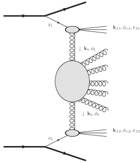
Figure 1: Schematical illustration of the kinematics.

Due to the large longitudinal momentum fractions $x_{J,1}$ and $x_{J,2}$ of the forward jets, collinear factorization holds and the differential cross section can be written as

$$\frac{{\rm d}\sigma\,}{{\rm d}|{\bf k}_{J,1}|\,{\rm d}|{\bf k}_{J,2}|\,{\rm d}y_{J,1}\,{\rm d}y_{J,2}\,}=\sum_{{\rm a},{\rm b}}\int_{0}^{1}{\rm d}x_{1}\,\int_{0}^{1}{\rm d}x_{2}\,f_{\rm a}(x_{1})f_{\rm b}(x_{2})\frac{{\rm d}{\hat{\sigma}}_{\rm{ab}}\,}{{\rm d}|{\bf k}_{J,1}|\,{\rm d}|{\bf k}_{J,2}|\,{\rm d}y_{J,1}\,{\rm d}y_{J,2}\,},$$ (1)

where $f_{\rm a,b}$ are the parton distribution functions (PDFs) of a parton a (b) in the according proton (which are renormalization scale $\mu_{R}$ and factorization scale $\mu_{F}$ dependent). The resummation of logarithmically enhanced contributions are included through $k_{T}$-factorization:

$$\frac{{\rm d}{\hat{\sigma}}_{\rm{ab}}\,}{{\rm d}|{\bf k}_{J,1}|\,{\rm d}|{\bf k}_{J,2}|\,{\rm d}y_{J,1}\,{\rm d}y_{J,2}\,}=\int{\rm d}\phi_{J,1}\,{\rm d}\phi_{J,2}\,\int{\rm d}^{2}{\bf k}_{1}\,{\rm d}^{2}{\bf k}_{2}\,V_{\rm a}(-{\bf k}_{1},x_{1})G({\bf k}_{1},{\bf k}_{2},{\hat{s}})V_{\rm b}({\bf k}_{2},x_{2}),$$ (2)

where the BFKL Green’s function $G$ depends on ${\hat{s}}=x_{1}x_{2}s$. The jet vertices $V_{a,b}$ were calculated at

NLL order in Ref. [13]. Combining the PDFs with the jet vertices one writes

$$\frac{{\rm d}\sigma\,}{{\rm d}|{\bf k}_{J,1}|\,{\rm d}|{\bf k}_{J,2}|\,{\rm d}y_{J,1}\,{\rm d}y_{J,2}\,} = \int{\rm d}\phi_{J,1}\,{\rm d}\phi_{J,2}\,\int{\rm d}^{2}{\bf k}_{1}\,{\rm d}^{2}{\bf k}_{2}\,\Phi({\bf k}_{J,1},x_{J,1},-{\bf k}_{1})\,G({\bf k}_{1},{\bf k}_{2},{\hat{s}})\,\Phi({\bf k}_{J,2},x_{J,2},{\bf k}_{2})\,$$

where $$\quad\Phi({\bf k}_{J,2},x_{J,2},{\bf k}_{2})=\int{\rm d}x_{2}\,f(x_{2})V({\bf k}_{2},x_{2}).$$ (3)

In view of the azimuthal decorrelation we want to investigate, we define the following coefficients:

$$\mathcal{C}_{m}\equiv\!\!\!\int\!\!{\rm d}\phi_{J,1}\,{\rm d}\phi_{J,2}\,\cos\big{(}m(\phi_{J,1}-\phi_{J,2}-\pi)\big{)}\!\!\!\int\!\!{\rm d}^{2}{\bf k}_{1}\,{\rm d}^{2}{\bf k}_{2}\,\Phi({\bf k}_{J,1},x_{J,1},-{\bf k}_{1})G({\bf k}_{1},{\bf k}_{2},{\hat{s}})\Phi({\bf k}_{J,2},x_{J,2},{\bf k}_{2}),$$

from which one can easily obtain the differential cross section and azimuthal decorrelation as

$$\frac{{\rm d}\sigma\,}{{\rm d}|{\bf k}_{J,1}|\,{\rm d}|{\bf k}_{J,2}|\,{\rm d}y_{J,1}\,{\rm d}y_{J,2}\,}=\mathcal{C}_{0}\quad{\rm and}\quad\langle\cos(m\varphi)\rangle\equiv\langle\cos\big{(}m(\phi_{J,1}-\phi_{J,2}-\pi)\big{)}\rangle=\frac{\mathcal{C}_{m}}{\mathcal{C}_{0}}.$$ (4)

The guiding principle is then to rely on the LL-BFKL eigenfunctions

$$E_{n,\nu}({\bf k}_{1})=\frac{1}{\pi\sqrt{2}}\left({\bf k}_{1}^{2}\right)^{i\nu-\frac{1}{2}}e^{in\phi_{1}}\,,$$ (5)

although they strictly speaking do not diagonalize the NLL BFKL kernel. In the LL approximation,

$$\mathcal{C}_{m}=(4-3\delta_{m,0})\int{\rm d}\nu\,C_{m,\nu}(|{\bf k}_{J,1}|,x_{J,1})C^{*}_{m,\nu}(|{\bf k}_{J,2}|,x_{J,2})\left(\frac{{\hat{s}}}{s_{0}}\right)^{{\omega}(m,\nu)}\,,$$ (6)

where

$$C_{m,\nu}(|{\bf k}_{J}|,x_{J})= \int{\rm d}\phi_{J}\,{\rm d}^{2}{\bf k}\,{\rm d}x\,f(x)V({\bf k},x)E_{m,\nu}({\bf k})\cos(m\phi_{J})\,,$$ (7)

and ${\omega}(n,\nu)={\bar{\alpha}}_{s}\chi_{0}\left(|n|,\frac{1}{2}+i\nu\right),$ with $\chi_{0}(n,\gamma)=2\Psi(1)-\Psi\left(\gamma+\frac{n}{2}\right)-\Psi\left(1-\gamma+\frac{n}{2}\right)$ and ${\bar{\alpha}}_{s}=N_{c}\alpha_{s}/\pi$. The master formulae of the LL calculation (6, 7) will also be used for the NLL calculation. The price to pay in order that $E_{n,\nu}$ remains eigenfunction is to accept that the eigenvalue become an operator containing a derivative with respect to $\nu$. In combination with the impact factors the derivative acts on the impact factors and effectively leads to a contribution to the eigenvalue

which depends on the impact factors.

At NLL, the jet vertices are intimately dependent on the jet algorithm  [13]. We here use the cone algorithm, which is expected to the used by the CMS collaboration. At NLL, one should also pay attention to the choice of scale $s_{0}$. We find the choice of scale $s_{0}=\sqrt{s_{0,1}\,s_{0,2}}$ with $s_{0,1}=\frac{x_{1}^{2}}{x_{J,1}^{2}}{\bf k}_{J,1}^{2}$ rather natural, since it does not depend on the momenta ${\bf k}_{1,2}$ to be integrated out. Besides, the dependence with respect to $s_{0}$ of the whole amplitude can be studied, when taking account the fact that both the NLL BFKL Green function and the vertex functions are $s_{0}$ dependent. In order to study the effect of possible collinear improvement [15, 16], we have, in a separate study, implemented for $n=0$ the scheme 3 of Ref. [15]. This is only required by the Green function since we could show by a numerical study that the jet vertices are free of $\gamma$ poles and thus do not call for any collinear improvement. In practice, the use of Eqs. (6, 7) leads to the possibility to calculate for a limited number of $m$ the coefficients $C_{m,\nu}$ as universal grids in $\nu$, instead of using a two-dimensional grid in ${\bf k}$ space. We use MSTW 2008 PDFs [17] and a two-loop strong coupling with a scale $\mu_{R}=\sqrt{|{\bf k}_{J,1}|\cdot|{\bf k}_{J,2}|}\,.$ Although a BFKL treatment does not require any asymmetry between the two emmited jets, in order to compare with DGLAP NLO approaches [18] obtained through the NLL-DGLAP partonic generator Dijet [19], for which symmetric configurations lead to instabilities, we here display our results for $|{\bf k}_{J,1}|=35\,{\rm GeV}$, $|{\bf k}_{J,2}|=50\,{\rm GeV}$, and compare them with the DGLAP NLO prediction (see Ref. [12] for symetric configurations).

3 Results

We now present our results for the LHC at the design center of mass energy $\sqrt{s}=14\,{\rm TeV}$. Motivated by a recent CMS study [14] we restrict the rapidities of the Mueller Navelet jets to the region $3<|y_{J}|<5$, thus limiting the relative rapidity $Y$ between 6 and 10 units. Fig. 2a and  2b respectively display the cross-section and the azimuthal correlation. This explicitely shows the dramatic effect of the NLL vertex corrections, of the same order as the one for the Green function. In particular, the decorrelation based on our full NLL analysis is very small, similar to the one based on NLO DGLAP.

\psfrag{varied}{}\psfrag{cubaerror}{}\psfrag{C0}{\raisebox{2.84544pt}{\footnotesize$\mathcal{C}_{0}\left[\frac{\rm nb}{{\rm GeV}^{2}}\right]=\sigma$}}\psfrag{Y}{$Y$}\includegraphics[width=142.26378pt]{michelc0.eps}

\psfrag{varied}{}\psfrag{cubaerror}{}\psfrag{C0}{\raisebox{2.84544pt}{\footnotesize$\mathcal{C}_{0}\left[\frac{\rm nb}{{\rm GeV}^{2}}\right]=\sigma$}}\psfrag{Y}{$Y$}\psfrag{C1C0}{\raisebox{2.84544pt}{\footnotesize$\frac{\mathcal{C}_{1}}{\mathcal{C}_{0}}=\langle\cos\varphi\rangle$}}\includegraphics[width=142.26378pt]{michelc1c0.eps}

Figure 2: Differential cross section and azimuthal correlation in dependence on $Y$ for $|{\bf k}_{J,1}|=35\,{\rm GeV}$, $|{\bf k}_{J,2}|=50\,{\rm GeV}$. The errors due to the Monte Carlo integration are given as error bands. As dots are shown the results of Ref. [18] obtained with Dijet [19].

The main source of uncertainties is due to the renormalization scale $\mu_{R}$ and to the energy scale $\sqrt{s_{0}}$.  This is particularly important for the azimuthal correlation, which,

when including a collinear improved Green’s function, may exceed 1 for small $\mu_{R}=\mu_{F}$.

In conclusion, contrarily to the general belief, the study of Mueller Navelet jets is probably not the best place to exhibit differences between BFKL and DGLAP dynamics.

Work supported in part by the Polish Grant N202 249235, the grant ANR-06-JCJC-0084 and by a PRIN grant (MIUR, Italy).

References

- [1] V. S. Fadin et al., Phys. Lett. B 60 (1975) 50; E. A. Kuraev et al., Sov. Phys. JETP 44 (1976) 443; Sov. Phys. JETP 45 (1977) 199; I. I. Balitsky and L. N. Lipatov, Sov. J. Nucl. Phys. 28 (1978) 822.
- [2] A. J. Askew et al., Phys. Lett. B 325 (1994) 212; H. Navelet et al., Phys. Lett. B 385 (1996) 357; S. Munier et al., Nucl. Phys. B 524 (1998) 377; J. Bartels et al., Phys. Lett. B 389 (1996) 742; S. J. Brodsky et al., Phys. Rev. Lett. 78 (1997) 803; [Erratum-ibid. 79 (1997) 3544]; A. Bialas et al., Eur. Phys. J. C 2 (1998) 683; M. Boonekamp et al., Nucl. Phys. B 555 (1999) 540; J. Kwiecinski and L. Motyka, Phys. Lett. B 462 (1999) 203. S. J. Brodsky et al., JETP Lett. 70 (1999) 155; S. J. Brodsky et al., JETP Lett. 76 (2002) 249 [Pisma Zh. Eksp. Teor. Fiz. 76 (2002) 306].
- [3] A. H. Mueller, Nucl. Phys. Proc. Suppl. 18C (1991) 125.
- [4] I. F. Ginzburg et al., Nucl. Phys. B 284 (1987) 685; Nucl. Phys. B 296 (1988) 569; M. G. Ryskin, Z. Phys. C 57 (1993) 89; A. H. Mueller and W. K. Tang, Phys. Lett. B 284 (1992) 123. D. Y. Ivanov et al., Phys. Rev. D 58 (1998) 114026; Phys. Lett. B 478 (2000) 101 [Erratum-ibid. B 498 (2001) 295]. B. Pire et al., Eur. Phys. J. C 44 (2005) 545; R. Enberg et al., Eur. Phys. J. C 45 (2006) 759 [Erratum-ibid. C 51 (2007) 1015]; M. Segond et al., Eur. Phys. J. C 52 (2007) 93; D. Y. Ivanov and A. Papa, Nucl. Phys. B 732 (2006) 183; Eur. Phys. J. C 49 (2007) 947; F. Caporale et al., Eur. Phys. J. C 53 (2008) 525.
- [5] V. N. Gribov et al., Sov. J. Nucl. Phys. 15 (1972) 438; L. N. Lipatov, Sov. J. Nucl. Phys. 20 (1975) 94; G. Altarelli et al., Nucl. Phys. B 126 (1977) 298; Y. L. Dokshitzer, Sov. Phys. JETP 46 (1977) 641.
- [6] A. H. Mueller and H. Navelet, Nucl. Phys. B 282 (1987) 727.
- [7] D0 Collaboration, B. Abbott et. al., Phys. Rev. Lett. 84 (2000) 5722.
- [8] V. Del Duca et al., Phys. Rev. D 49 (1994) 4510; W. J. Stirling, Nucl. Phys. B 423 (1994) 56.
- [9] L. H. Orr et al., Phys. Rev. D 56 (1997) 5875; J. Kwiecinski et al., Phys. Lett. B 514 (2001) 355.
- [10] V. S. Fadin et al., Phys. Lett. B 429 (1998) 127; M. Ciafaloni et al., Phys. Lett. B 430 (1998) 349.
- [11] A. Sabio Vera et al., Nucl. Phys. B 776 (2007) 170; C. Marquet et al., Phys. Rev. D 79 (2009) 034028.
- [12] D. Colferai, F. Schwennsen, L. Szymanowski and S. Wallon, arXiv:1002.1365 [hep-ph].
- [13] J. Bartels, D. Colferai, and G. P. Vacca, Eur. Phys. J. C 24 (2002) 83; 29 (2003) 235.
- [14] CMS Collaboration, S. Cerci and D. d’Enterria, AIP Conf. Proc. 1105 (2009) 28.
- [15] G. P. Salam, JHEP 07 (1998) 019.
- [16] M. Ciafaloni et al., Phys. Lett. B 452 (1999) 372; Phys. Rev. D 60 (1999) 114036; Phys. Rev. D 68 (2003) 114003.
- [17] A. D. Martin, W. J. Stirling, R. S. Thorne and G. Watt, Eur. Phys. J. C 63 (2009) 189.
- [18] M. Fontannaz, LPT-Orsay/09-86 (2009).
- [19] P. Aurenche, R. Basu, and M. Fontannaz, Eur. Phys. J. C 57 (2008) 681.